Underwater Side-Scan Sonar Target Detection: An Enhanced YOLOv11 Framework Integrating Attention Mechanisms and a Bi-Directional Feature Pyramid Network

Abstract

Underwater target detection is pivotal for marine exploration, yet it faces significant challenges because of the inherent complex underwater environment. Sonar images are generally degraded by noise, exhibit low resolution, and lack prominent target features, making the extraction of useful feature information from blurred and complex backgrounds particularly challenging. These limitations hinder highly accurate autonomous target detection in sonar imagery. To address these issues, this paper proposes the ABFP-YOLO model, which was designed to enhance the accuracy of underwater target detection. Specifically, the bi-directional feature pyramid network (BiFPN) structure is integrated into the model to efficiently fuse the features of different scales, significantly improving the capability of the network to recognize targets of varying scales, especially small targets in complex scenarios. Additionally, an attention module is incorporated to enhance feature extraction from blurred images, thereby boosting the detection accuracy of the model. To validate the proposed model’s effectiveness, extensive comparative and ablation experiments were conducted on two datasets. The experimental results demonstrate that the ABFP-YOLO model achieves mean average precision (mAP0.5) scores of 0.988 and 0.866, indicating its superior performance in target detection tasks within complex underwater environments.

1. Introduction

The introduction of the “21st Century Maritime Silk Road” initiative has created both significant development opportunities and new challenges for marine surveying and mapping [1,2,3,4]. As the fundamental basis for all marine development activities [2,5,6], seafloor target detection represents one of the most critical tasks in this field [7,8,9]. With the integration of advanced technologies, this domain has undergone rapid progress, playing an indispensable role in national defense, marine engineering, and scientific research. Amidst escalating international competition, security concerns in coastal regions have become increasingly prominent. Emerging underwater threats characterized by stealth, intelligence, and miniaturization, such as naval mines, combat divers, and unmanned underwater vehicles, pose latent risks to critical infrastructure, including harbors, docks, and military installations. As a result, research on intelligent underwater target detection technology holds substantial strategic importance.

While deep learning approaches have been extensively used in target detection domains [10,11], most existing approaches are specifically designed for optical imagery, exhibiting limited generalization capabilities when applied to side-scan sonar datasets. Side-scan sonar imagery is characterized by less prominent features and sparse target distribution. In contrast, optical imaging systems, primarily designed for terrestrial feature recognition, exploit rich texture patterns and distinct contour information to achieve high detection accuracy. Although side-scan sonar provides high-resolution seafloor topography mapping, it differs significantly from optical imaging modalities in terms of technical characteristics [12]. The inherent limitations of side-scan sonar data further exacerbate detection challenges: (1) Acoustic backscatter signals from targets exhibit minimal contrast against background seabed sediments. (2) Surface texture details are poorly represented due to the nature of acoustic imaging mechanisms. (3) The sparse spatial distribution of underwater targets introduces additional identification complexity. These fundamental differences between side-scan sonar target detection tasks and optical image analysis significantly hinder the direct implementation of conventional deep learning-based detection frameworks in marine acoustic applications.

Target detection encompasses both target recognition and localization. Traditional target interpretation in side-scan sonar imagery is predominantly based on manual methods that are inefficient, time-consuming, and highly subjective [13]. To address these limitations, researchers have explored automatic detection methods using machine learning approaches based on traditional feature extraction and classification [14,15,16,17]. For example, Tang et al. [18] proposed a transfer learning recognition method based on an improved VGG-16 framework, achieving automatic identification of shipwrecks with significantly higher precision and efficiency compared to traditional methods. Nguyen et al. [19] trained a GoogleNet model using side-scan sonar images augmented through scattering, polarization, and geometric transformations, achieving a 91.6% recognition accuracy value for drowning victims. Feldens et al. [20] employed RetinaNet to detect individual rocks on the seabed surface. Tang et al. [21] implemented shipwreck detection using the YOLOv3 network with transfer learning. Yu et al. [22] enhanced the YOLOv5 model by incorporating an attention mechanism module, achieving high-precision shipwreck detection. Rutledge et al. [23] proposed a method for the detection of potential underwater archeological sites by means of autonomous underwater vehicles (AUVs). Topple et al. [24] introduced a mine-like target detection method for AUVs using the MiNet model, which features a smaller backbone structure and fewer parameters compared to the YOLO model. In summary, while these methods have made significant strides in achieving intelligent underwater target detection, challenges persist due to the severe noise in sonar images, indistinct target features, and low image resolution. Existing deep learning methods still face limitations including poor feature extraction, the neglect of correlations among convolutional features, significant interference from background noise, and lengthy model training times. These issues hinder the rapid and accurate detection and localization of targets in side-scan sonar imagery.

To address the issues of inconspicuous and sparsely distributed features in side-scan sonar imaging, improve the network’s ability to learn about objects, and extract useful feature information from blurred images with complex backgrounds, this paper proposes the ABFP-YOLO model to improve the accuracy and real-time performance of underwater target detection. The proposed model integrates two key innovations: First, the BiFPN structure is incorporated into the Neck of the network to efficiently fuse multi-scale features. BiFPN achieves weighted fusion of multi-level features through top-down and bottom-up bidirectional pathways, significantly enhancing feature representation. This bidirectional multi-scale feature integration enhances the network’s detection capability for targets of varying scales, particularly for small targets in complex scenarios. Second, the attention module is introduced and applied to the neural network to improve feature extraction from blurred images. By leveraging channel attention and spatial attention mechanisms, the attention mechanism strengthens the focus of the network on salient features while suppressing irrelevant or noisy features, thereby improving the recognition accuracy of the model. Experimental findings show that the ABFP-YOLO model effectively improves both the precision and real-time efficiency in underwater target detection, offering an innovative approach to the challenge of poor detection precision caused by the inconspicuous and sparsely distributed features in side-scan sonar imaging.

2. Materials and Methods

2.1. Attention Mechanism Module

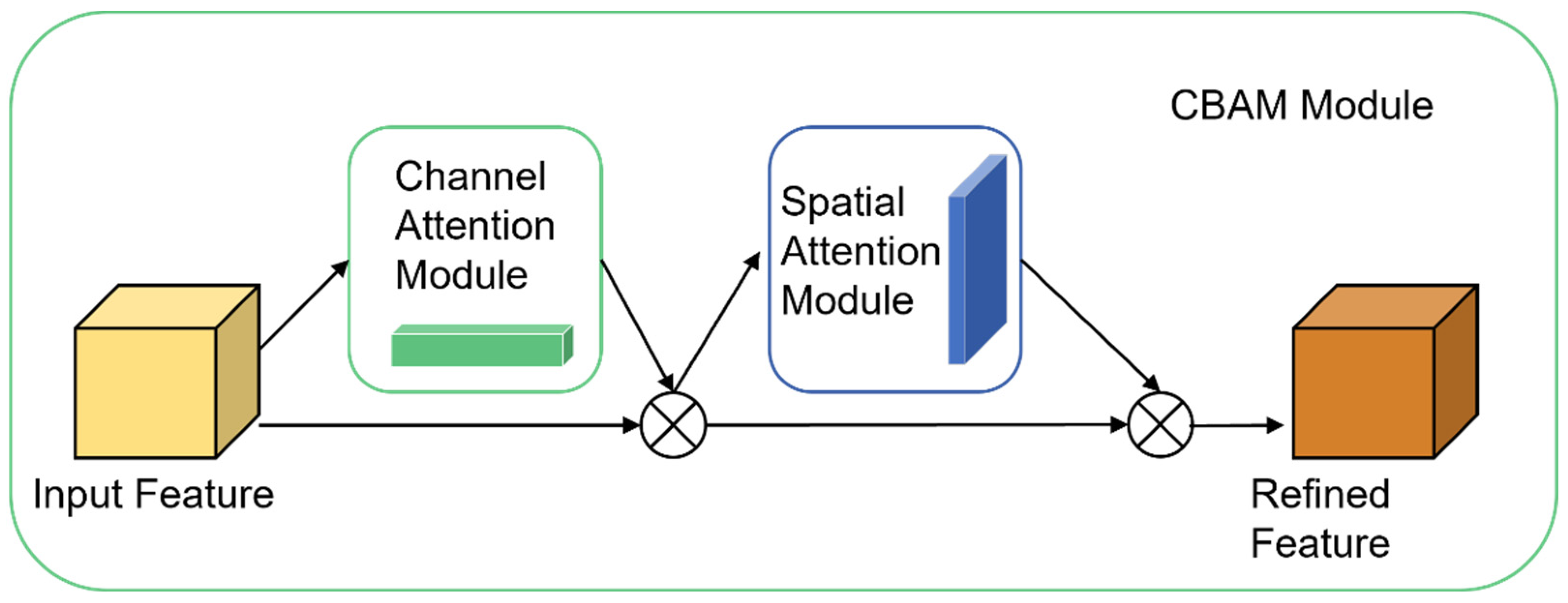
An advanced attention mechanism tailored for convolutional neural networks (CNNs) is the convolutional block attention module (CBAM). It improves feature representation by integrating dual attention mechanisms: channel attention and spatial attention. As illustrated in Figure 1, CBAM consists of two key components: the Channel Attention Module (CAM) and the Spatial Attention Module (SAM). This modular design allows CBAM to be seamlessly integrated into various positions within the network without compromising computational efficiency. In contrast to attention mechanisms that prioritize either spatial or channel dimensions individually, CBAM achieves enhanced performance by effectively combining both aspects, thereby optimizing feature extraction and representation.

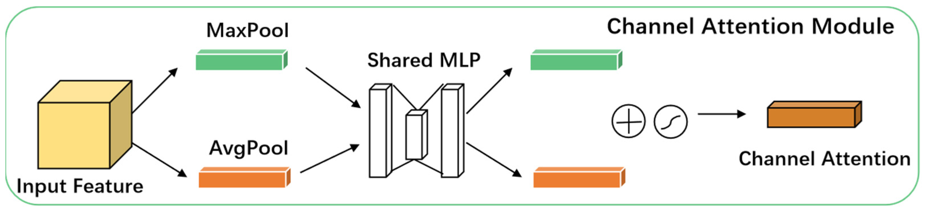
The CAM, as depicted in Figure 2, is designed to learn interdependencies among channels by computing importance weights for each channel, thereby adjusting the response of individual channels within the feature map. This mechanism allows for the prioritization of the most informative feature channels by the network, greatly improving feature representation. The implementation of CAM involves the following steps:

Global Max Pooling and Global Average Pooling: Global max pooling and global average pooling operations are applied to each channel of the input feature map. These operations extract the maximum and average feature values per channel, respectively, generating two vectors that encapsulate the global maximum and average features across all channels.

Fully Connected Layer: A common fully connected (FC) layer passes the feature vectors derived from global max pooling and global average pooling. This FC layer allows the network to adaptively identify the most relevant channels for the task by learning attention weights for each channel. The outputs from the global max and average pooling paths are combined to produce the final attention weight vector.

Sigmoid Activation: A sigmoid activation function is applied to the combined output of the FC layer to normalize the attention weights between 0 and 1. This produces the channel attention weights, which quantify the importance of each channel.

Attention Weighting: Attention weighting multiplies the calculated attention weights by corresponding the channels of the original feature map. This results in an attention-weighted feature map, where task-relevant channels are amplified, while less relevant channels are attenuated.

On the other hand, the SAM, as depicted in Figure 3, emphasizes the spatial relationships by calculating importance weights at each spatial location. This mechanism enables the network to prioritize the most significant spatial positions, enhancing spatial feature representation. The implementation of SAM involves the following steps:

Max Pooling and Average Pooling: Max pooling and average pooling operations are applied to the input feature map along the dimension of the channel. These operations generate features that capture different contextual scales, providing complementary information about the spatial structure.

Concatenation and Convolution: The features derived from max pooling and average pooling operations are concatenated along the channel dimension, creating a feature map that integrates contextual information from multiple scales. This concatenated feature map is then processed through a convolutional layer in order to generate spatial attentional weights.

Sigmoid Activation: A sigmoid activation function is applied to the spatial attention weights to normalize them between 0 and 1. This step produces the final spatial attention weights, which quantify the importance of each spatial location.

Attention Weighting: The calculated spatial attention weights are applied to an original feature map to weight features at each spatial location. This step amplifies the relevant parts of the image while attenuating the influence of less relevant areas.

2.2. BiFPN Network Architecture

The feature pyramid network (FPN) is a network architecture that integrates the multi-resolution scale prediction of a single-shot multibox detector (SSD) with the multi-resolution feature fusion of U-Net. To better adapt to target image characteristics and task requirements, the architecture has evolved from simple feature addition to complex feature fusion pyramids.

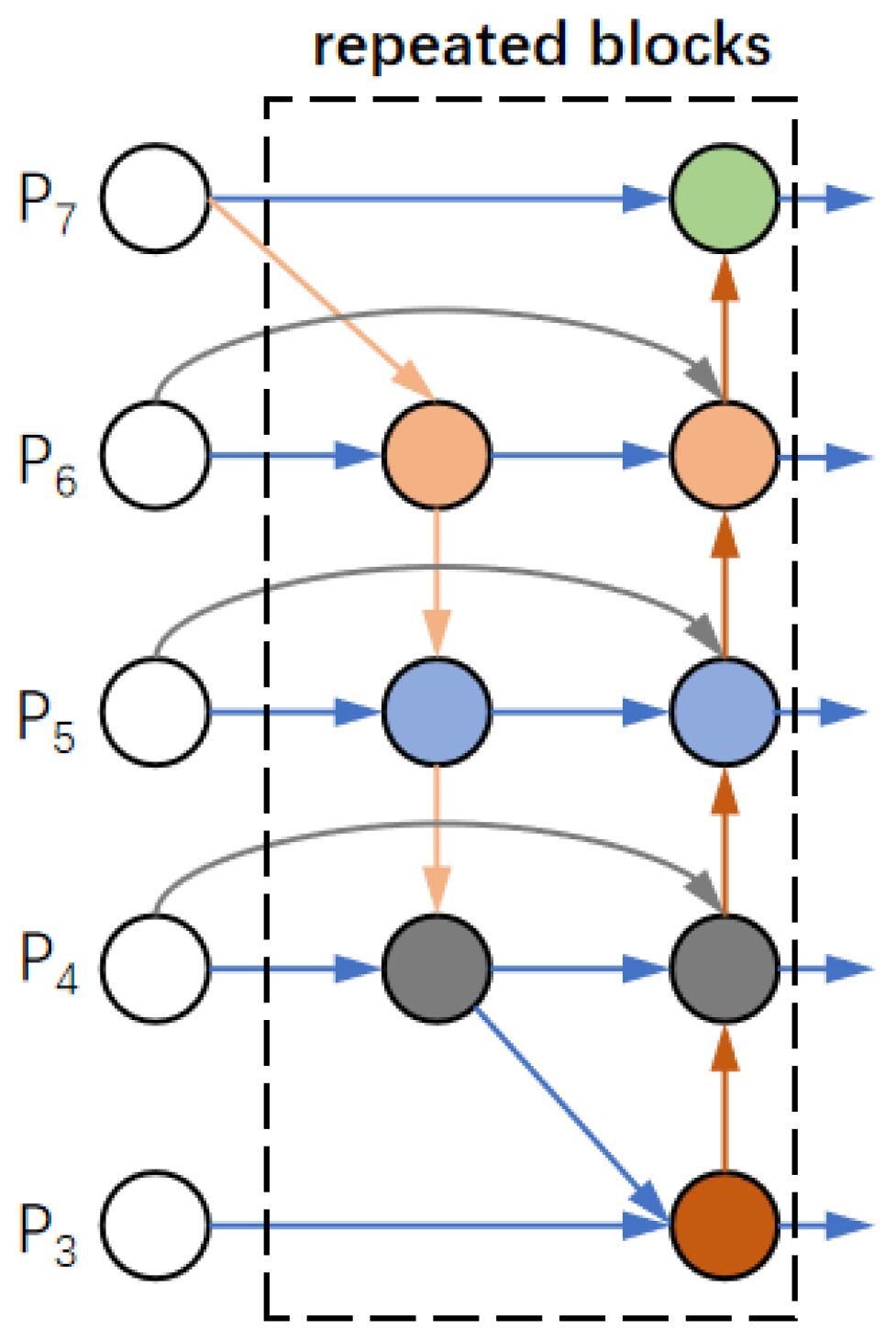
The BiFPN introduced by Tan et al. in EfficientDet [25] enables efficient multi-scale feature fusion. This network incorporates a composite feature map scaling strategy, allowing for the uniform scaling of resolution, depth, and width across the backbone network, feature network, and final predictive network. To understand the multi-scale feature fusion problem, multi-scale features can be formally represented as follows:

$${\overrightarrow{P}}^{in}=\left(P_{l_1}^{in},P_{l_2}^{in},\dots \right)$$

(1)

where $P_{l_1}^{in}$ represents the feature at pixel $l_1$. A transformation $f$ that is capable of effectively integrating diverse features and generating refined output features exists, satisfying the following:

$${\overrightarrow{P}}^{out}=f\left({\overrightarrow{P}}^{in}\right)$$

(2)

In the traditional FPN, the top-down fusion of multi-scale features is expressed as follows:

$$\left\{\begin{array}{c}{P}_7^{out}=Conv\left(P_7^{in}\right)\\ P_6^{out}=Conv\left(P_6^{in}+Resize\left(P_7^{out}\right)\right)\\ \dots \\ P_3^{out}=Conv\left(P_3^{in}+Resize\left(P_4^{out}\right)\right)\end{array}\right.$$

(3)

where $Resize$ represents the upsampling and downsampling operations for resolution matching and conv denotes the convolutional operation for feature information processing. In traditional FPN, feature fusion across different layers is critically important, and researchers have proposed various approaches to address this challenge. For instance, the Path Aggregation Network (PANet) enhances the representational capacity of the backbone network by fusing both bottom-up and top-down pathways [26], while the Neural Architecture Search Feature Pyramid Network (NAS-FPN) employs neural architecture search to optimize the topological structure of multi-scale feature networks [27]. To further improve model efficiency, the BiFPN adopts a cross-scale connection method with the following formulation:

(1)

Remove some input nodes: Nodes with fewer input edges often contribute minimally to feature fusion due to their lower weights. To simplify computations, these nodes are removed.

(2)

Add skip connections: As input and output nodes at identical scales are situated within the same layer, skip connections are added to enable additional feature fusion without increasing computational overhead.

(3)

Merge bidirectional path network layers: To achieve higher-level feature fusion, network layers with bidirectional communication are merged and repeated during each activation.

When fusing image features at different resolutions, they are typically resized to the same resolution for integration. The feature pyramid attention network incorporates a global self-attention upsampling method to restore pixel localization, a technique subsequently refined in NAS-FPN. Prior to BiFPN, all input features were treated equally, despite the fact that features with different resolutions often contribute unequally to the output features. BiFPN addresses this limitation by assigning an additional weight to each input, enabling the network to learn the relative importance of each feature. As shown in Figure 4, BiFPN combines bidirectional cross-scale connections with fast normalized fusion, optimizing feature fusion across scales.

2.3. Novel Network Architecture

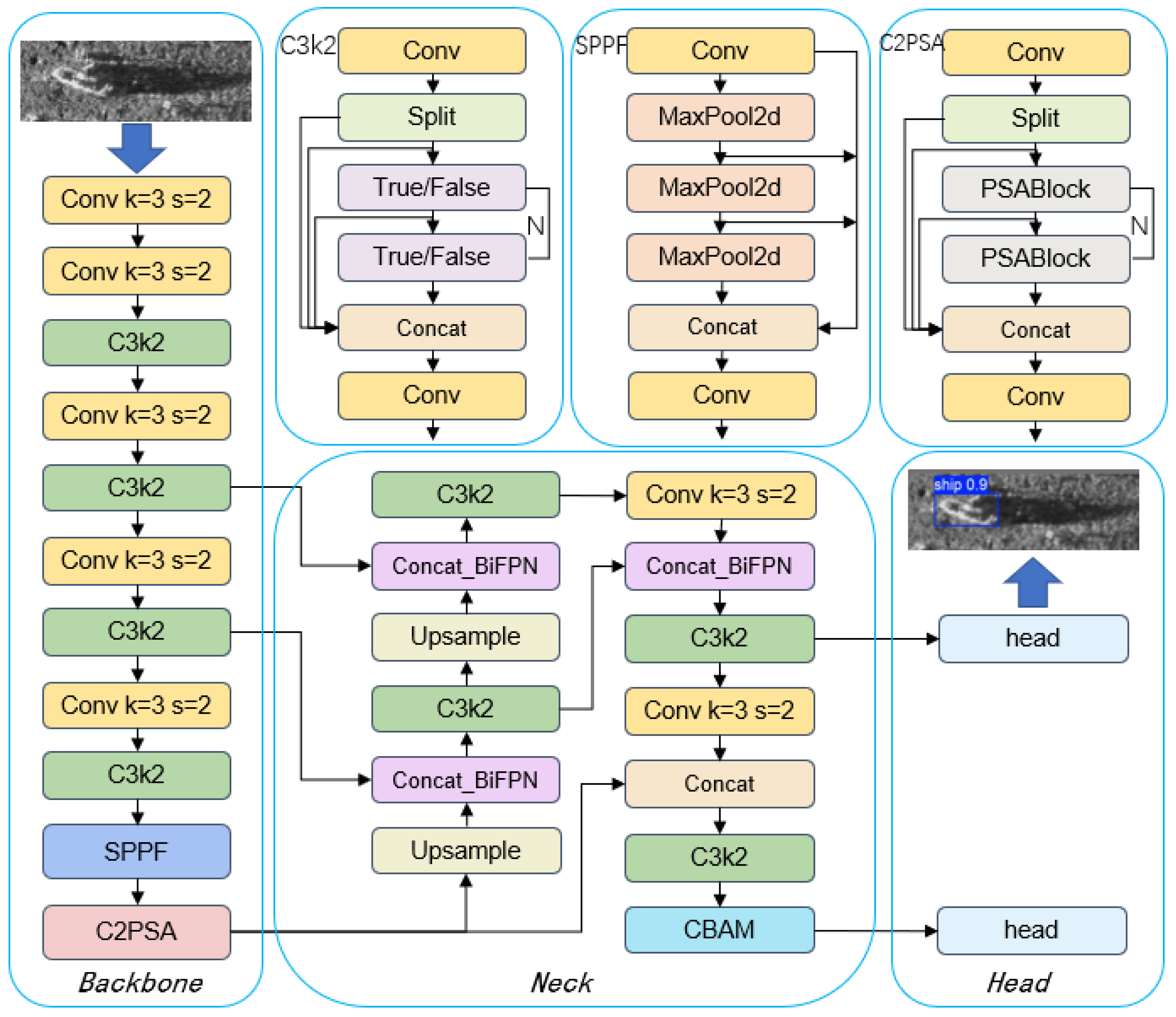
To enhance the network’s learning capability for targets, extract useful feature information from blurred images with complex backgrounds, and address the challenges posed by inconspicuous and sparsely distributed features in side-scan sonar imaging, this study introduces an innovative target detection algorithm named ABFP-YOLO, whose architectural framework is depicted in Figure 5.

In our approach, the BiFPN structure is integrated into the Neck of the network to efficiently fuse multi-scale features. BiFPN achieves weighted fusion of multi-level features through top-down and bottom-up bidirectional pathways, significantly enhancing feature representation. Furthermore, this bidirectional multi-scale feature fusion enhances the network’s ability to detect targets of varying scales, particularly for small targets in complex scenarios.

Additionally, the CBAM is applied to the neural network. By leveraging the mechanisms of channel attention and spatial attention, CBAM strengthens the network’s focus on important features while suppressing interference from irrelevant features, thus improving the detection accuracy of the model.

The deep learning model architecture comprises three core components: a backbone, Neck, and Head. The backbone section includes multiple convolutional layers, C3k2 modules, SPPF modules, and C2PSA modules, which are designed to extract image features. The Neck section performs multi-scale feature fusion using BiFPN and further processes features through upsampling and C3k2 modules. The Head section incorporates CBAMs and final convolutional layers to generate predictions. The model achieves efficient image processing through multiple convolutional operations, feature fusion, and attention mechanisms.

3. Experiment and Results

3.1. Datasets

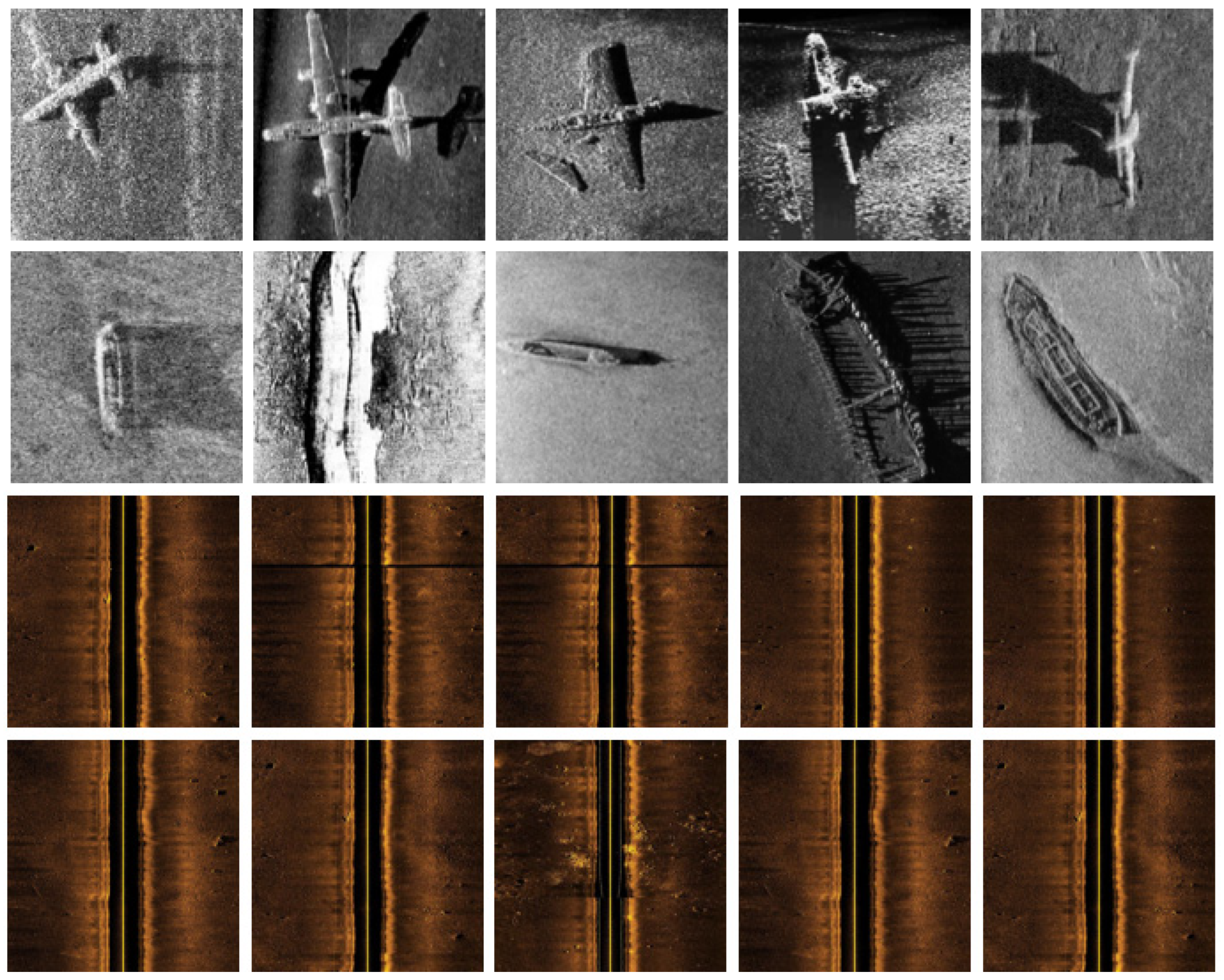
Two datasets were employed in the experiments conducted for this study. The first dataset is the publicly available KLSG dataset, while the second dataset comprises side-scan sonar data collected by the Portuguese Navy’s Sappers Diver Group Number Three (Destacamento de Mergulhadores Sapadores—DMS 3) in 2015. The first dataset comprises two classes: ships and an aircraft, with a sum of 447 images. Specifically, it contains 395 targets of the ship category and 62 targets of the aircraft category. The second dataset includes two categories: non-mine-like bottom objects (NOMBOs) and mine-like contacts (MILCOs), totaling 240 images. Within this dataset, NOMBOs appear 175 times, and MILCO objects appear 238 times. We then conduct preprocessing on images, which involves normalization and data augmentation.

The hardware configuration for model training consisted of an Intel^® CoreTM i5-13500H CPU (Lenovo of China, Wuhan, China) and an NVIDIA GeForce RTX 4050 graphics processor with 6 GB of memory. The operating environment included Python 3.11.7, CUDA 11.8, and PyTorch 2.1.2 running on Windows 11. Figure 6 provides a visual representation of a subset of the dataset employed in this study.

3.2. Evaluation Metrics

This study employs five primary metrics to evaluate model performance. Precision (P) quantifies the ratio of accurately predicted positive instances to the total number of instances classified as positive. It measures the predictive accuracy of the model, with higher precision indicating fewer false positives (FPs) in positive predictions. The formula for the calculation is given in Equation (4). Recall (R) indicates the percentage of actual positive instances correctly identified by the model. The calculation formula is given in Equation (5). The mean average precision at IoU = 0.5 (mAP0.5) represents the average precision (AP) calculated at an intersection over union (IoU) threshold of 0.5, averaged across all classes. The corresponding calculation formula is provided in Equation (6). The mean average precision at IoU = 0.5:0.95 (mAP0.5:0.95) calculates AP across multiple IoU values ranging from 0.5 to 0.95 (in increments of 0.05), then averages these values across all classes. The calculation formula is provided in Equation (7).

$$Precision={\displaystyle \frac{TP}{TP+FP}}$$

(4)

where TP (true positive) corresponds to accurately identified positive samples, and FP (false positive) refers to misclassified positive samples.

$$Recall={\displaystyle \frac{TP}{TP+FN}}$$

(5)

where FN (false negative) represents incorrectly classified negative samples; TP + FP denotes the sum of positive samples; and TP + FN indicates the sum of the classified samples.

$$mAP0.5={\displaystyle \frac{1}{N}}\sum _{i=1}^N{AP}_i (ioU=0.5)$$

(6)

where N denotes the number of classes and ${AP}_i$ denotes the average accuracy for the i-th category. The mAP0.5 metric, one of the most commonly used evaluation indicators in object detection, comprehensively considers both precision and recall while assessing localization accuracy through an IoU threshold of 0.5. A higher mAP0.5 value reflects superior model performance in detection tasks.

$$mAP0.5:0.95={\displaystyle \frac{1}{N}}\sum _{i=1}^N({\displaystyle \frac{1}{M}}\sum _{j=1}^{M}A{P}_{ij})$$

(7)

where N represents the total number of classes, M signifies the total number of IoU thresholds (typically 10, ranging from 0.5 to 0.95), and ${AP}_{i,j}$ indicates the average accuracy for category i at threshold j. The mAP0.5:0.95 metric serves as a more rigorous evaluation criterion, as it demands that the model retains high detection performance across varying IoU thresholds. A higher mAP0.5:0.95 value demonstrates stronger robustness and accuracy in both localization and classification tasks.

3.3. Small Target Detection Performance Evaluation

3.3.1. KLSG Dataset Results

Quantitative Results on the KLSG Dataset

We conducted underwater target detection experiments using the KLSG dataset (ships and aircraft) to evaluate the performance of multiple object detection models, including YOLOv5, YOLOv11, FFCA-YOLO, L-FFCA-YOLO, and our proposed model. To ensure experimental consistency, all models were tested with identical input dimensions of 640 × 640. The results, summarized in

Table 1. Quantitative evaluation of experimental results on the KLSG dataset.

Model	Input Shape	Parameters (M)	GFLOPs	Precision	Recall	mAP0.5	mAP0.5:0.95	Time/h
YOLOv5	640 × 640	7.02	15.8	91.6%	79.4%	0.907	0.551	0.209
YOLOv11	640 × 640	2.58	6.3	94.7%	86%	0.945	0.758	0.741
FFCA-YOLO [28]	640 × 640	0.70	8.2	92.8%	87.4%	0.957	0.714	9.072
L-FFCA-YOLO [28]	640 × 640	0.64	7.7	83.8%	93%	0.95	0.598	7.859
ours	640 × 640	2.55	5.3	92.5%	98.1%	0.988	0.894	0.615

, include key metrics like parameters, Giga Floating-point Operations Per Second (GFLOPs), precision, recall, mean average precision (map0.5), extended mean average precision (mAP0.5:0.95), and runtime.

First, in terms of parameters and GFLOPs, the model proposed in this paper demonstrates relatively good performance in terms of computational complexity, indicating that it has significantly enhanced computational efficiency through structural optimization. Compared with the existing YOLOv5, YOLOv11, FFCA–YOLO, and L–FFCA–YOLO models, although its parameter quantity is not the lowest, there is a notable reduction in computational complexity. In particular, when compared with YOLOv5 and FFCA–YOLO, it shows higher computational efficiency. This can likely be attributed to the optimization and design improvements of the model structure, enabling it to maintain good performance while reducing the consumption of computational resources.

From the perspective of precision and recall, YOLOv11 demonstrates optimal performance, achieving a precision of 94.7% and a recall of 86%. This indicates that the model exhibits high precision and comprehensiveness in target identification. Nevertheless, our proposed model shows particularly outstanding performance in recall, reaching 98.1%, which signifies its superior effectiveness in detecting targets within images. Although its precision is slightly lower than YOLOv11 at 92.5%, this result highlights the significant advantage of our model in terms of detection comprehensiveness.

Regarding mAP0.5 and mAP0.5:0.95, our model also demonstrates exceptional performance. It reaches 0.988 mAP0.5 and 0.894 mAP0.5:0.95, surpassing other models in both metrics. This indicates that our model maintains high detection accuracy across different IoU thresholds, demonstrating strong robustness. In comparison, while L-FFCA-YOLO achieves an mAP0.5 of 0.95, its mAP0.5:0.95 is only 0.598, revealing limitations in detection capability at higher IoU thresholds.

Finally, from the perspective of runtime, YOLOv5 shows optimal performance with a runtime of 0.209 h, demonstrating its advantage in real-time detection tasks. However, our model maintains a relatively short runtime of 0.615 h while preserving high detection accuracy, significantly outperforming FFCA-YOLO and L-FFCA-YOLO in efficiency. This indicates that our model not only ensures detection precision but also sustains good real-time performance, making it suitable for practical target detection applications.

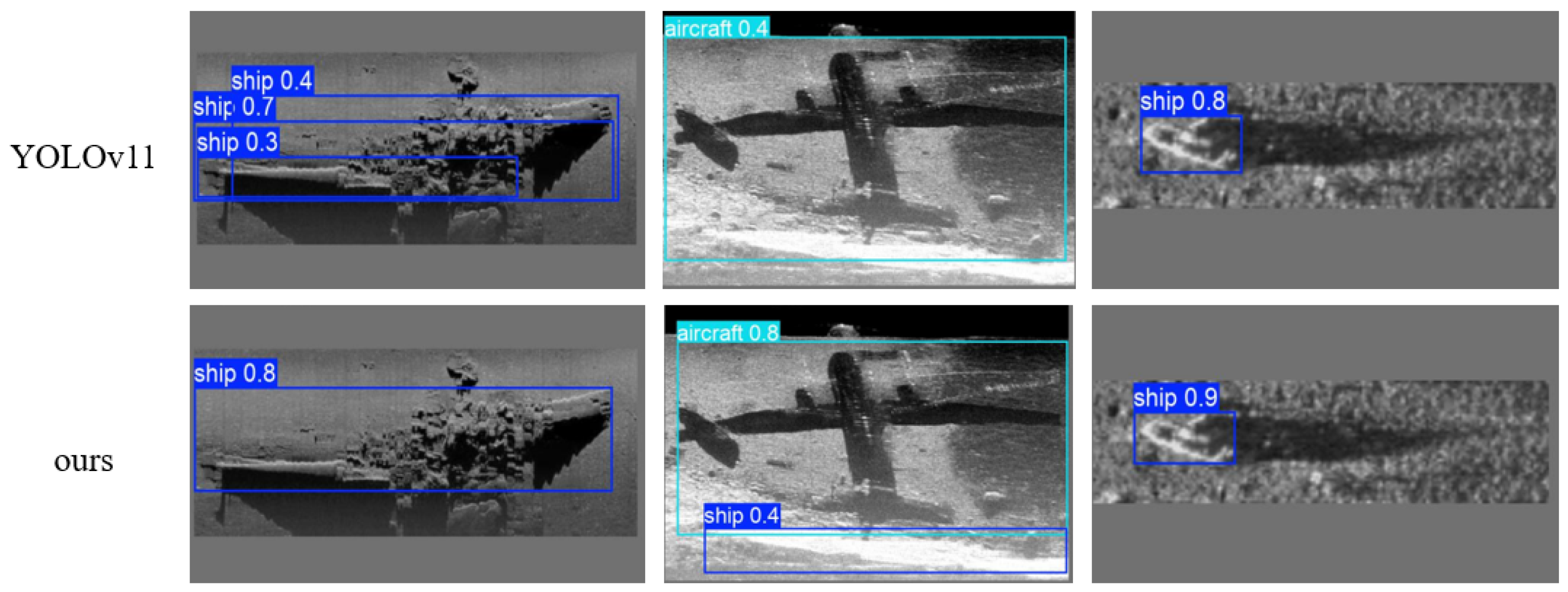
Qualitative Results on the KLSG Dataset

To provide a clear visual representation of the detection performance across various algorithms, we conducted a qualitative comparative analysis of YOLOv11 and our proposed method in target detection tasks.

As shown in Figure 7, our method exhibits significant advantages in both detection accuracy and robustness. First, for ship target detection, YOLOv11 produces multiple overlapping bounding boxes in the first image, indicating challenges in handling targets within complex backgrounds. In contrast, our method accurately identifies the ship and provides a precise bounding box, demonstrating higher precision and robustness in processing such targets. Second, for aircraft target detection, while YOLOv11 successfully identifies the aircraft in the second image, the position and size of its bounding box are not entirely accurate, and it fails to detect the shipwreck, which could impact subsequent recognition tasks. Our method, however, accurately identifies both the aircraft and the shipwreck, providing precise bounding boxes, which highlights its superior accuracy and robustness in handling such targets.

3.3.2. SSS-Bottom Data Results

Quantitative Results on SSS-Bottom Data

Experiments were performed utilizing the SSS-Bottom data, and the results are summarized in

Table 2. Quantitative evaluation of experimental results on SSS-Bottom Data.

Model	Input Shape	Parameters (M)	GFLOPs	Precision	Recall	mAP0.5	mAP0.5:0.95	Time/h
YOLOv5	640 × 640	7.02	15.8	78.1%	82.6%	0.752	0.425	0.465
YOLOv11	640 × 640	2.58	6.3	79.1%	89.4%	0.868	0.623	0.994
FFCA-YOLO	640 × 640	0.70	8.2	67.6%	91.9%	0.798	0.483	0.947
L-FFCA-YOLO	640 × 640	0.64	7.7	69.8%	73.3%	0.708	0.419	0.67
ours	640 × 640	2.55	5.3	96.8%	81.8%	0.866	0.63	0.465

.

First, in terms of precision, our proposed model performed the best, achieving 96.8% and significantly outperforming other models. YOLOv11 and YOLOv5 followed closely with precisions of 79.1% and 78.1%, respectively, while FFCA-YOLO and L-FFCA-YOLO had relatively lower precisions of 67.6% and 69.8%. This indicates that our model has a clear advantage in target recognition accuracy. In terms of recall, FFCA-YOLO performed the best, achieving 91.9%, demonstrating its strength in comprehensive target detection. However, our model also performed well in recall, achieving 81.8%, second only to FFCA-YOLO. YOLOv11 and YOLOv5 achieved recalls of 89.4% and 82.6%, respectively, while L-FFCA-YOLO had a recall of 73.3%. This shows that our model can effectively detect most targets while maintaining high precision. Regarding mAP0.5 and mAP0.5:0.95, our model also performed excellently, achieving scores of 0.866 and 0.63, respectively, which were slightly higher than YOLOv11’s 0.868 and 0.623. YOLOv5 achieved an mAP0.5 and an mAP0.5:0.95 of 0.752 and 0.425, respectively, while FFCA-YOLO and L-FFCA-YOLO achieved 0.798 and 0.483, and 0.708 and 0.419, respectively. This further confirms the superior comprehensive performance of our model. Finally, in terms of training time, our model was closest to YOLOv5, both requiring 0.465 h, demonstrating its efficiency in training. YOLOv11, FFCA-YOLO, and L-FFCA-YOLO required training times of 0.994 h, 0.947 h, and 0.67 h, respectively, indicating that our model maintains high performance while also being highly efficient in training.

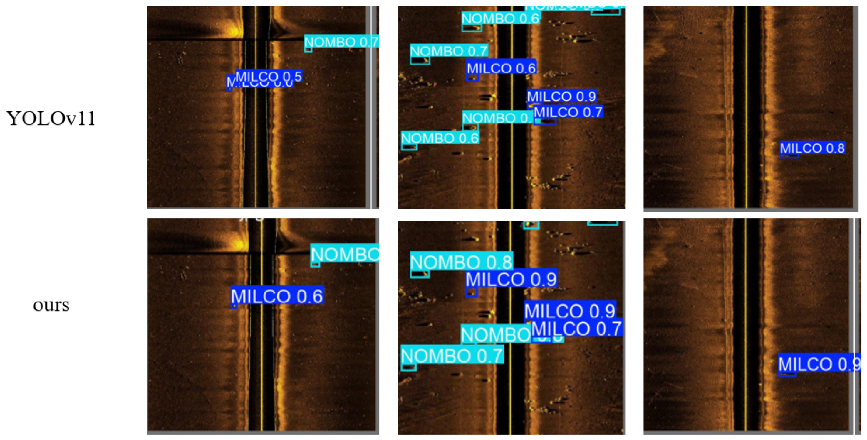
Qualitative Results on SSS-Bottom Data

To visually demonstrate the detection results of different algorithms, we conducted a qualitative comparative analysis between YOLOv11’s performance and our proposed method in the object detection task.

From Figure 8, it can be observed that YOLOv11 has certain limitations in detection accuracy. In the first column of images, although YOLOv11 can detect the target, its confidence score is only 0.5, indicating insufficient accuracy in target recognition. In the second column of images, the detection results of YOLOv11 show some improvement, but there are still multiple instances of false detections, further highlighting its limited detection capability in complex scenarios. In the third column of images, the detection results of YOLOv11 are relatively accurate, but the confidence score is only 0.8, indicating some uncertainty in target recognition.

In contrast, our proposed method demonstrates significant advantages in the object detection task. In the first column of images, our method accurately detects the target with a confidence score of 0.6, indicating more precise target recognition. In the second column of images, our method not only accurately detects the target but also effectively avoids false detections, further demonstrating its stronger detection capability in complex scenarios. In the third column of images, the detection results of our method are not only accurate but also achieve a confidence score of 0.9, indicating higher certainty in target recognition. Therefore, our proposed method exhibits significant advantages in the object detection task, with higher detection accuracy and stronger robustness.

3.4. Ablation Study

To validate the role played by each module in the performance of the model, an ablation study was conducted using the evaluation metrics of parameters, GFLOPs, precision, recall, mAP0.5, and mAP0.5:0.95. The study focused on the CBAM and the BiFPN. Four experimental groups were designed, as summarized in

Table 3. Quantitative results of the ablation study on the KLSG dataset.

Model	CBAM	BiFPN	Input Shape	Parameters (M)	GFLOPs	Precision	Recall	mAP0.5	mAP0.5:0.95
1	-	-	640 × 640	2.58	6.3	94.7%	86%	0.945	0.758
2	√	-	640 × 640	2.59	6.3	93.7%	96.4%	0.964	0.873
3	-	√	640 × 640	2.58	6.3	95.2%	96%	0.961	0.838
4	√	√	640 × 640	2.55	5.3	92.5%	98.1%	0.988	0.894

.

The baseline model does not incorporate the CBAM or Concat_BiFPN modules. It achieves a precision of 94.7%, a recall of 86%, an mAP0.5 of 0.945, and an mAP0.5:0.95 of 0.758. These results indicate that the baseline model performs well in precision and mAP0.5 but relatively poorly in recall and mAP0.5:0.95. This may be due to the lack of effective feature fusion and attention mechanisms, leading to limitations in complex scenarios or small object detection tasks.

Model 2 introduces the CBAM to the baseline model. Its precision slightly decreases to 93.7%, but its recall significantly improves to 96.4%, mAP0.5 increases to 0.964, and mAP0.5:0.95 increases to 0.873. These results demonstrate that the CBAM improves the model’s capacity to concentrate on important features, significantly improving recall and mAP0.5:0.95. Although precision slightly decreases, the overall performance is significantly improved, particularly in complex scenarios, where the model demonstrates greater robustness.

Model 3 introduces the BiFPN module to the baseline model. Its precision increases to 95.2%, recall improves to 96%, mAP0.5 increases to 0.961, and mAP0.5:0.95 increases to 0.838. Compared to the baseline model, the introduction of the BiFPN module substantially improves precision and recall, indicating that this module effectively fuses multi-scale features and boosts the model’s detection ability. However, the improvement in mAP0.5:0.95 is relatively modest, suggesting that the BiFPN module has a limited impact on comprehensive detection performance.

Model 4 incorporates both the CBAM and BiFPN modules. It achieves a precision of 92.5%, and its recall significantly improves to 98.1%, mAP0.5 increases to 0.988, and mAP0.5:0.95 increases to 0.894. These results demonstrate that the combined use of the CBAM and BiFPN modules significantly enhances recall and mAP0.5:0.95, particularly excelling in complex scenarios. Although precision slightly decreases, the significant improvements in recall and mAP0.5:0.95 indicate that the model has a notable advantage in reducing missed detections and improving comprehensive detection capabilities. Model 4 achieves a significant reduction in GFLOPs while reducing the number of parameters, indicating an improvement in computational efficiency.

4. Discussion

Performance Under Different CBAM Configurations

This study investigates the impact of the CBAM on object detection model performance by comparing the YOLOv11 model’s efficacy under different CBAM configurations. The experimental findings reveal that the introduction of CBAM markedly improves the model’s detection performance, but its effectiveness is closely related to the number of CBAMs, as summarized in

Table 4. Performance under different CBAM configurations.

Model	CBAM Number	Input Shape	Precision	Recall	mAP0.5	mAP0.5:0.95
YOLOv11	0	640 × 640	94.7%	86%	0.945	0.758
YOLOv11	1	640 × 640	93.7%	96.4%	0.964	0.873
YOLOv11	2	640 × 640	92.6%	95.3%	0.962	0.775
YOLOv11	3	640 × 640	89.1%	96.3%	0.955	0.743

.

When no CBAM is used, the YOLOv11 model achieves a precision of 94.7%, a recall of 86%, an mAP0.5 of 0.945, and an mAP0.5:0.95 of 0.758. These results indicate that the baseline model performs well in precision and mAP0.5 but relatively poorly in recall and mAP0.5:0.95. This may be attributed to the lack of an effective attention mechanism, resulting in limitations in complicated scenarios or small object detection tasks.

When one CBAM is introduced, the model’s precision slightly decreases to 93.7%, but its recall significantly improves to 96.4%, mAP0.5 increases to 0.964, and mAP0.5:0.95 increases to 0.873. These results demonstrate that a single CBAM strengthens the model’s capacity to concentrate on crucial features, significantly improving recall and mAP0.5:0.95. Although precision slightly decreases, the overall performance is significantly improved, particularly in complex scenarios, where the model demonstrates greater robustness.

When the number of CBAMs increases to two, the model’s precision further decreases to 92.6%, and its recall is 95.3%, mAP0.5 is 0.962, and mAP0.5:0.95 is 0.775. Compared to CBAM = 1, recall and mAP0.5 slightly decrease, while mAP0.5:0.95 shows a more noticeable decline. This suggests that increasing the number of CBAMs may lead to diminishing marginal returns, as excessive attention modules may increase model complexity, resulting in feature redundancy or overfitting.

When the number of CBAMs increases to three, the model’s precision significantly decreases to 89.1%, and its recall is 96.3%, mAP0.5 is 0.955, and mAP0.5:0.95 is 0.743. These results indicate that an excessive number of CBAMs negatively impact model performance, particularly in precision and mAP0.5:0.95. This may be due to the fact that an excessive number of attention modules hinder model convergence during training, or the attention mechanism overly focuses on certain features while neglecting other important information.

An appropriate number of CBAMs (e.g., CBAM = 1) can provide the best performance improvement, while an excessive number may lead to performance degradation. Therefore, in practical applications, the number of CBAMs should be chosen based on specific task requirements to balance model performance and complexity.

5. Conclusions

To improve the network’s capability to learn targets and extract valuable feature information from blurred images with intricate backgrounds, this study addresses the challenges of side-scan sonar imaging, where features are often indistinct and sparsely distributed. We propose the ABFP-YOLO model to improve the accuracy and real-time performance of underwater target detection. The BiFPN structure is integrated into the Neck of the network to efficiently fuse multi-scale features, significantly enhancing the network’s ability to detect targets of varying scales, particularly small targets in complex scenarios. Additionally, the CBAM is introduced and applied to the neural network to strengthen feature extraction from blurred images. Our enhanced model demonstrates that the introduction of the CBAM and BiFPN modules significantly improves recall and mAP0.5:0.95, especially in complex scenarios and small target detection tasks, where the model exhibits greater robustness. The combined use of these modules further enhances the model’s comprehensive detection capabilities. Extensive experimental validation effectively establishes the accuracy and generalization ability of the proposed model. Furthermore, we discuss the performance under different CBAM configurations. An appropriate number of CBAMs (e.g., CBAM = 1) can provide the best performance improvement, while an excessive number may lead to performance degradation. Therefore, in practical applications, the number of CBAMs should be chosen based on specific task requirements to balance model performance and complexity. In future work, we will continue to optimize the network model for underwater target recognition to improve detection speed. Additionally, we will further improve the image quality of underwater scanning images and enrich the dataset to enable the model to adapt to more diverse underwater scenarios, thereby advancing the application of this model in specialized underwater environments with AI technologies.