Underwater Time Delay Estimation Based on Meta-DnCNN with Frequency-Sliding Generalized Cross-Correlation

Abstract

In underwater signal processing, accurate time delay estimation (TDE) is of crucial importance for ensuring the reliability of data transmission. However, the complex propagation of sound waves and strong noise interference in the underwater environment make this task extremely challenging. Especially under the condition of low signal-to-noise ratio (SNR), the existing methods based on cross-correlation and deep learning struggle to meet requirements. Aiming at this core issue, this paper proposed an innovative solution. Firstly, a multi-sub-window reconstruction is performed on the frequency-sliding generalized colorboxpinkcross-correlation (FS-GCC) matrix between signals to capture the time delay characteristics from different frequency bands and conduct the enhancement and extraction of features. Then, the grayscale image corresponding to the generated FS-GCC matrix is used, and the multi-level noise features are extracted by the multi-layer convolution of denoising convolutional neural network (DnCNN), effectively suppressing the noise and improving the estimation accuracy. Finally, the model-agnostic meta-learning (MAML) framework is introduced. Through training tasks under various SNR conditions, the model is enabled to possess the ability to quickly adapt to new environments, and it can achieve the desired estimation accuracy even when the number of underwater training samples is limited. Simulation validation was conducted under the NOF and NCS underwater acoustic channels, and results demonstrate that our proposed approach exhibits lower estimation errors and greater stability compared with existing methods under the same conditions. This method enhances the practicality and robustness of the model in complex underwater environments, providing strong support for the efficient and stable operation of underwater sensor networks.

1. Introduction

Underwater sensor networks [1,2], as a crucial technology for obtaining ocean information, are crucial for ocean detection, environmental monitoring, and military applications. Accurate underwater signal time delay estimation (TDE) is the foundation for ensuring the reliability of data transmission. It is related to whether a network can accurately and promptly acquire and transmit ocean information. In the complex underwater environment, acoustic wave propagation is affected by factors like water temperature, salinity, and depth, along with various noise sources such as marine organisms, ships, and waves. These conditions pose significant challenges to TDE, which are more pronounced than in terrestrial environments [3,4,5]. Therefore, improving the accuracy of underwater TDE is essential for the efficient and stable operation of underwater sensor networks.

The generalized cross-correlation (GCC) algorithm [6,7,8] is a vital tool for underwater TDE and is widely employed in scenarios such as detection, localization, and tracking of underwater targets. This algorithm estimates the time delay between two signals through frequency domain analysis, leveraging the phase information of the cross-power spectrum. Jang et al. [9] employed the GCC algorithm to extract the time difference of arrival (TDOA) information. By assigning specific weights to different frequency components, they effectively suppressed the noise interference and thus achieved the positioning and tracking of marine organisms. The uniqueness of this method lies in its frequency weighting technique, which can carry out targeted suppression according to the frequency characteristics of the noise. However, it has limited adaptability to complex and changeable noise environments. When the frequency distribution of the noise is relatively wide and irregular, the suppression effect will decline. Jia et al. [10] proposed an innovative zero-padding GCC algorithm for direct and reflected waves, accurately estimating time delays from unknown emission waveforms of underwater high-level explosive sound sources. However, this method is only applicable to specific sound sources, and its applicability to non-explosive sound sources needs to be further improved. Additionally, Pang et al. [11] proposed a TDE algorithm based on the quadratic GCC for the field of underwater positioning. This method conducts a quadratic GCC based on traditional weighting functions. Although the accuracy of time delay estimation has been improved under low signal-to-noise ratio (SNR) conditions, it still cannot effectively solve the problems of false peaks and spurious peaks caused by traditional weighting functions.

Although the GCC algorithm and its derivative methods have met the requirements of some underwater TDE to a certain extent, their susceptibility to noise remains a significant concern. Particularly in scenarios with low SNRs, the GCC algorithm is prone to generating spurious peaks, which can severely disrupt the accuracy of TDE, causing significant deviations between the estimated results and the actual values, and thus failing to meet the high-precision requirements of practical underwater applications. In recent years, with the rapid development of deep learning technology, there has been an increasing exploration of its applications in fields such as cross-correlation TDE and sound source localization [12,13]. Yao et al. [14] utilized parallel long short-term memory (LSTM) neural networks to estimate parameters in the GCC_PHAT model. By leveraging the LSTM’s strong ability to process time series data, this method effectively reduced the variance of TDE in low SNRs. However, the training process of this method is rather complicated, requiring a large amount of training data and a long training time. Salvati et al. [15] constructed a GCC feature matrix using PHAT filters with different parameters $\beta$, which was then input into a CNN to directly estimate the TDOA for speaker localization. The innovation of this method lies in the ingenious construction of the feature matrix of the GCC function. Nevertheless, due to the limited amount of underwater environment data, an insufficient dataset may lead to unsatisfactory training results. Comanducci et al. [16] employed GCCs as inputs and introduced a ray space transformation (RST) as an intermediary between CNN input and output, enhancing interpretability through feature visualization. However, this method has a relatively high computational complexity, and in a complex underwater environment, the stability of the RST intermediate quantity may be affected.

Despite that methods combining correlation functions with deep learning has shown strong generalization capabilities in the field of speech signal processing, underwater environments often suffer from low SNR due to environmental noise and reverberation, limiting the efficacy of these methods. To further enhance the robustness of TDE, the frequency-sliding generalized cross-correlation (FS-GCC) technique [17,18] has emerged. By applying subband low-pass filtering to the phase spectrum of the cross-power spectrum, this method provides a well-organized two-dimensional depiction of time delay data over various frequency ranges. Song et al. [19] extracted the principal eigenvectors of the FS-GCC through constructing window groups, pruning, deconvolution, and merging operations. A large number of experiments have verified that this algorithm outperforms other algorithms, such as having a lower estimating anomaly probability, lower estimation error, and a higher first-to-second peak ratio (FSPR). However, the adaptability of this method to certain extremely complex noise environments still needs to be further verified. Overall, this method provides new ideas and directions for the field of TDE. Subsequent research can be further optimized and improved on this basis to better address various challenges in practical applications. Recent research has combined FS-GCC with deep learning to address the TDE problem. For instance, Comanducci et al. [20] were inspired by deep learning image denoising approaches, proposing the use of U-Net to denoise images constructed from FS-GCC matrices, resulting in enhanced time delay information. However, the U-Net model still has room for improvement in the feature extraction ability of images.

To address these challenges, this paper proposes a meta-learning-based denoising convolutional neural network (DnCNN) FS-GCC method, named Meta-DnCNN_FS-GCC. This method takes the grayscale image generated by the feature-enhanced FS-GCC matrices as input to estimate the FS-GCC under noise-free conditions and optimize the accuracy of TDE. It aims to enhance signal processing capabilities in underwater environments, providing more reliable and accurate time delay information for underwater communication nodes.

The main contributions of this paper are as follows:

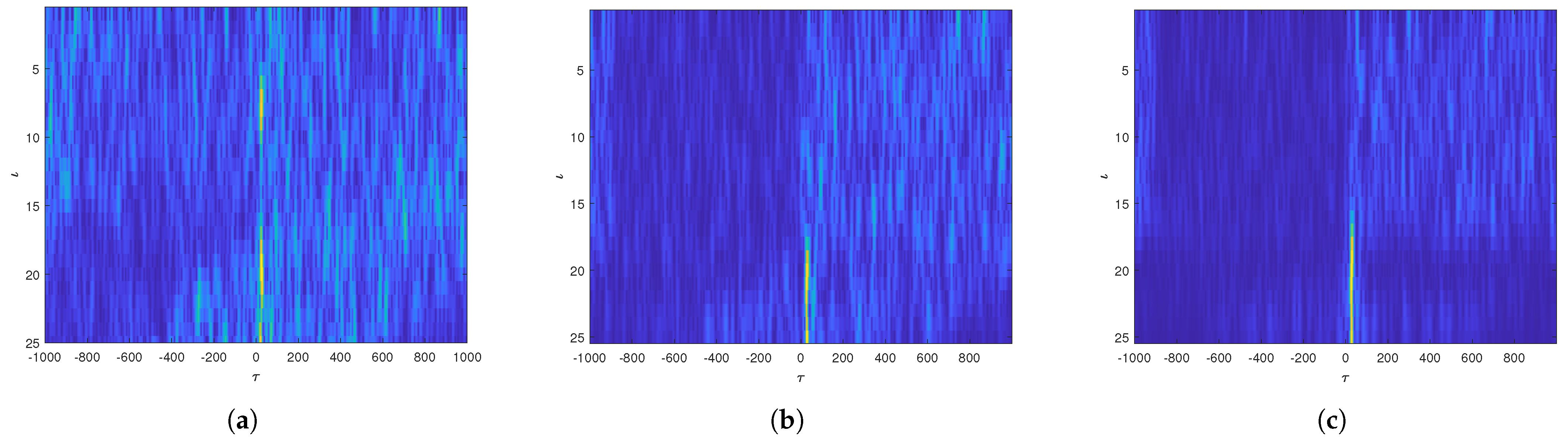
• Reconstruct FS-GCC matricies for multiple subwindow groups. Each subwindow captures time delay-related signal features from different frequency band perspectives, thereby enriching the information dimension of the FS-GCC matricies and enhancing the key feature vectors. Compared with traditional FS-GCC procedure, this reconstruction operation can more fully extract the time delay information in the signals, improve the accuracy of TDE, and reduce the probability of abnormal estimation.
• Recognizing the effectiveness of the DnCNN in image denoising and feature extraction, this paper introduces it into the field of underwater TDE. The FS-GCC matrix is transformed into a grayscale image, and the DnCNN architecture is utilized to strengthen time delay features reconstructed from the FS-GCC. The network automatically learns and extracts refined time delay features through multi-layer convolution operations, effectively suppressing noise interference and significantly improving estimation accuracy. Compared with other deep learning methods, DnCNN has stronger noise extraction capabilities and can better adapt to the complex underwater noise environment.
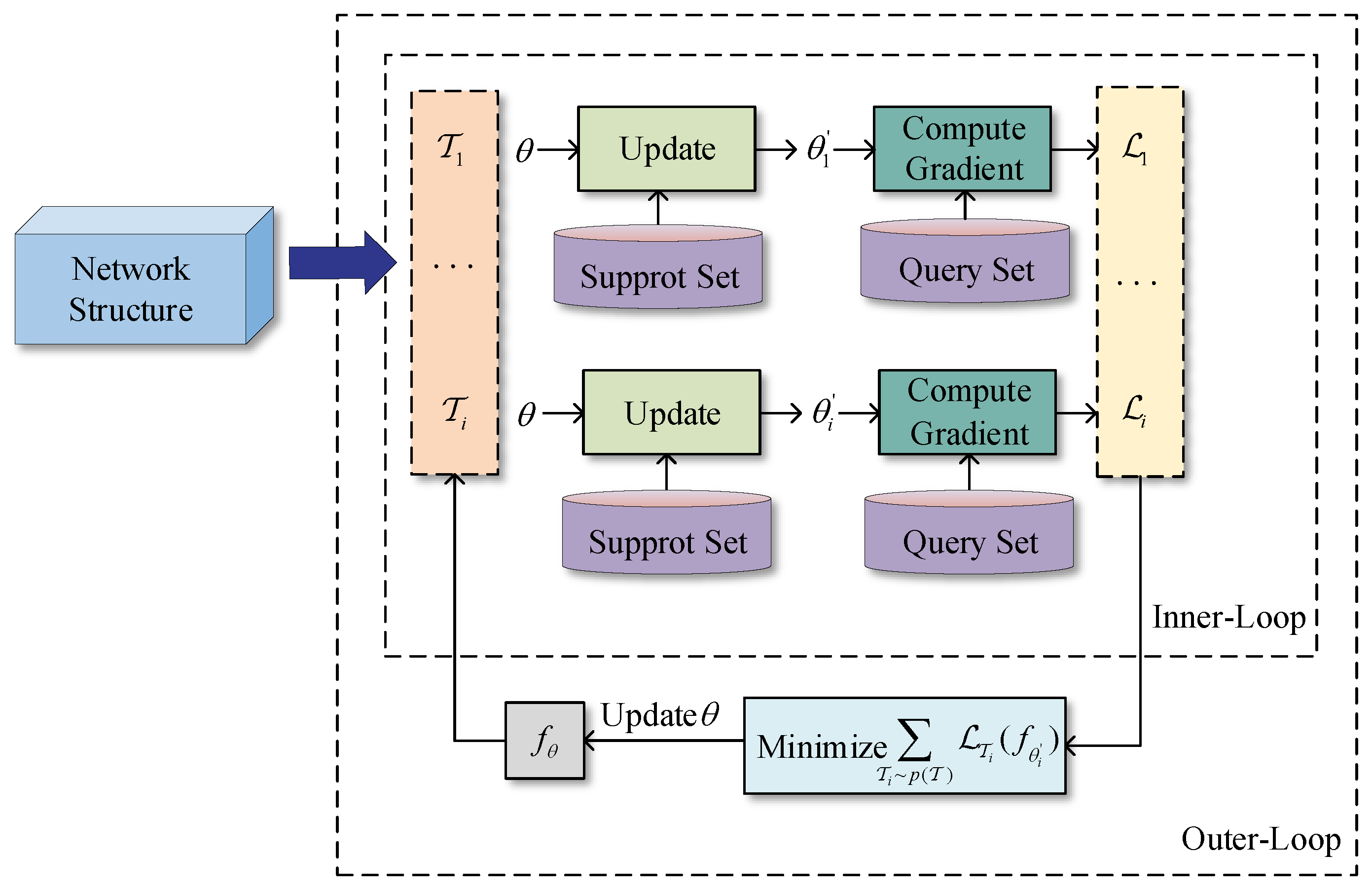
• Considering the variable SNR in underwater acoustic environments and the scarcity of high-quality training samples due to equipment limitations, we train the DnCNN model using a model-agnostic meta-learning (MAML) framework [21,22,23]. MAML simulates training tasks under diverse SNR conditions, enabling the model to adapt swiftly to new environments. This approach facilitates efficient learning with limited samples and promotes knowledge sharing across tasks, consequently increasing the model’s generalization ability in varying SNR scenarios and improving its practicality and robustness in complex underwater environments.

2. Basic Theory

2.1. Signal Model

A commonly used signal model for the classical TDE problem [19] is as in Equations (1) and (2):

$$x_1\left(t\right)=s_1\left(t\right)+n_1={\alpha }_{1}s(t-{\tau }_1)+n_1\left(t\right)$$

(1)

$$x_1\left(t\right)=s_2\left(t\right)+n_2={\alpha }_{2}s(t-{\tau }_2)+n_2\left(t\right)$$

(2)

where $x_1\left(t\right)$ and $x_2\left(t\right)$ represent the signals received by hydrophones 1 and 2, respectively. $s_1\left(t\right)$ and $s_2\left(t\right)$ are the noise-free signals, while $s\left(t\right)$ is the source signal. ${\alpha }_1$ and ${\alpha }_2$ denote the attenuation factor due to distance and material absorption. $n_1\left(t\right)$ and $n_2\left(t\right)$ represent the additive environmental noise. It is assumed that $s\left(t\right)$ and noise are uncorrelated. ${\tau }_1$ and ${\tau }_2$ denote the TDOA from the source to the hydrophone arrays.

The aforementioned equation can be converted into the discrete-time Fourier transform domain:

$$X_1\left(\omega \right)=S_1\left(\omega \right)+N_1\left(\omega \right)={\alpha }_{1}S\left(\omega \right)e^{-j\omega {\tau }_1}+N_1\left(\omega \right)$$

(3)

$$X_2\left(\omega \right)=S_2\left(\omega \right)+N_2\left(\omega \right)={\alpha }_{2}S\left(\omega \right)e^{-j\omega {\tau }_2}+N_2\left(\omega \right)$$

(4)

where $X_1\left(\omega \right)$, $X_2\left(\omega \right)$, $S_1\left(\omega \right)$, $S_2\left(\omega \right)$, $S\left(\omega \right)$, $N_1\left(\omega \right)$, and $N_2\left(\omega \right)$ are the Fourier transforms of $x_1\left(t\right)$, $x_2\left(t\right)$, $s_1\left(t\right)$, $s_2\left(t\right)$, $s\left(t\right)$, $n_1\left(t\right)$ and $n_2\left(t\right)$, respectively. $\omega$ is the normalized angular frequency by the sampling rate. $e^{-j\omega {\tau }_i}$ is the phase factor introduced by the time delay ${\tau }_i$, where $i=1,2$.

To effectively distinguish multi-path components, the transmitted signal needs to exhibit high time resolution. This paper employs Linear Frequency Modulation (LFM) signals, which feature a frequency that changes linearly with time. LFM signals possess substantial energy and bandwidth, making them resistant to noise interference [24]. The LFM signal is defined as

$$s\left(t\right)=Asin\left(2\pi (f_{0}t+{\displaystyle \frac{1}{2}}k{t}^2)\right)$$

(5)

where $A$ represents the signal amplitude, $k={\displaystyle \frac{B}{T}}$ represents the modulation rate of the LFM signal, $B$ represents the bandwidth, $T$ represents the time width, and $f_0$ represents the center frequency. The time-domain and frequency-domain representations of the signal are shown in Figure 1.

2.2. Generalized Cross-Correlation

The cross-power spectrum $G\left(\omega \right)$ of the phase transformation between signals $X_1\left(\omega \right)$ and $X_2\left(\omega \right)$ is defined as

$$G\left(\omega \right)=X_1\left(\omega \right)X_2^{*}\left(\omega \right)$$

(6)

where ${(·)}^{*}$ denotes the complex conjugate. The weighting function of GCC_PHAT is defined as

$$\psi \left(\omega \right)={\displaystyle \frac{1}{\left|G\right(\omega \left)\right|}}$$

(7)

GCC is the inverse Fourier transform of the weighted cross-power spectrum, represented as

$$R\left[\tau \right]={\displaystyle \frac{1}{2\pi }}{\int }_{-\pi }^{\pi }G\left(\omega \right)\psi \left(\omega \right)e^{j\omega \tau }d\omega$$

(8)

where $\tau$ denotes the time delay. Thus, the TDE based on GCC_PHAT is represented as

$$\widehat{\tau }=arg\underset{\tau }{max}R\left[\tau \right]$$

(9)

When accounting for noise and reverberation, GCC will exhibits spurious peaks, which complicates the TDE.

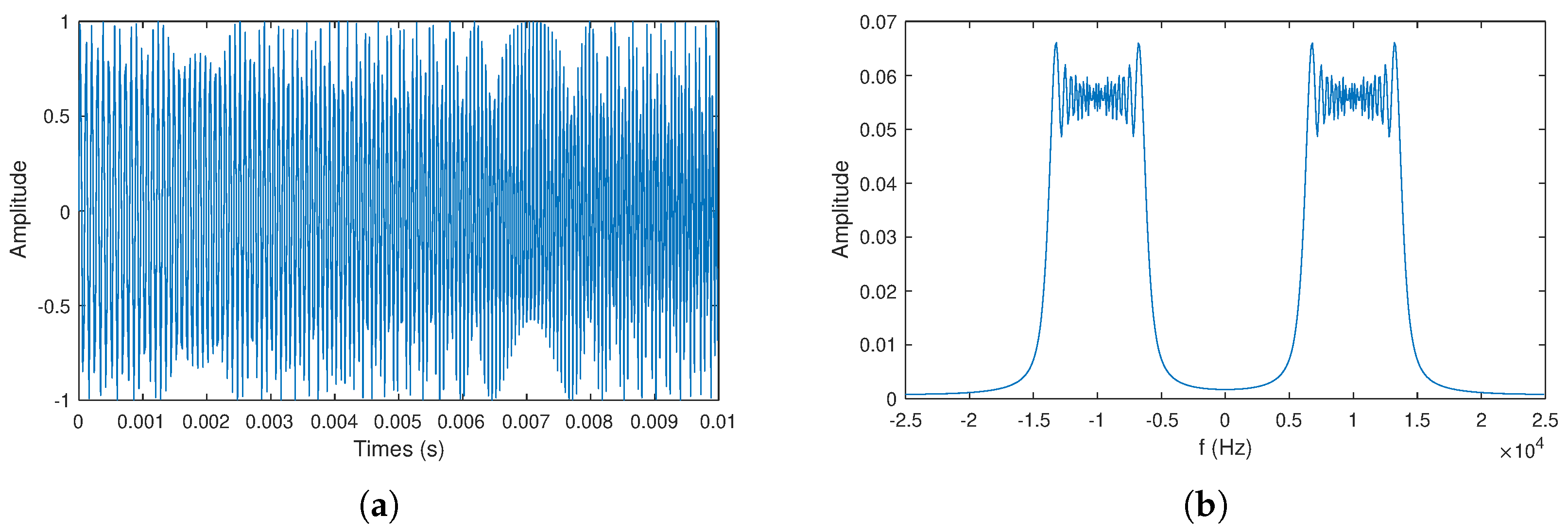
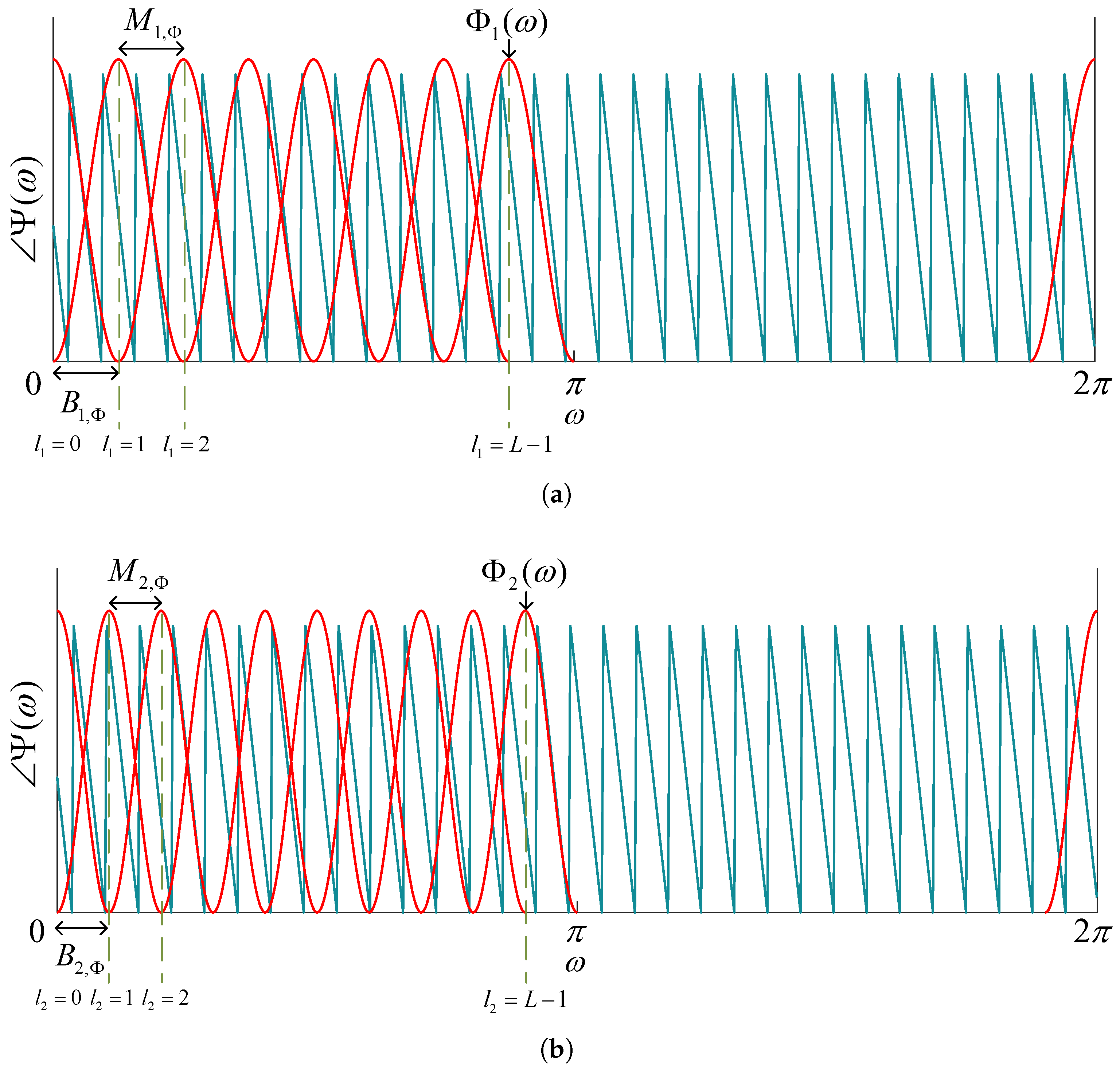
2.3. Frequency-Sliding Generalized Cross-Correlation

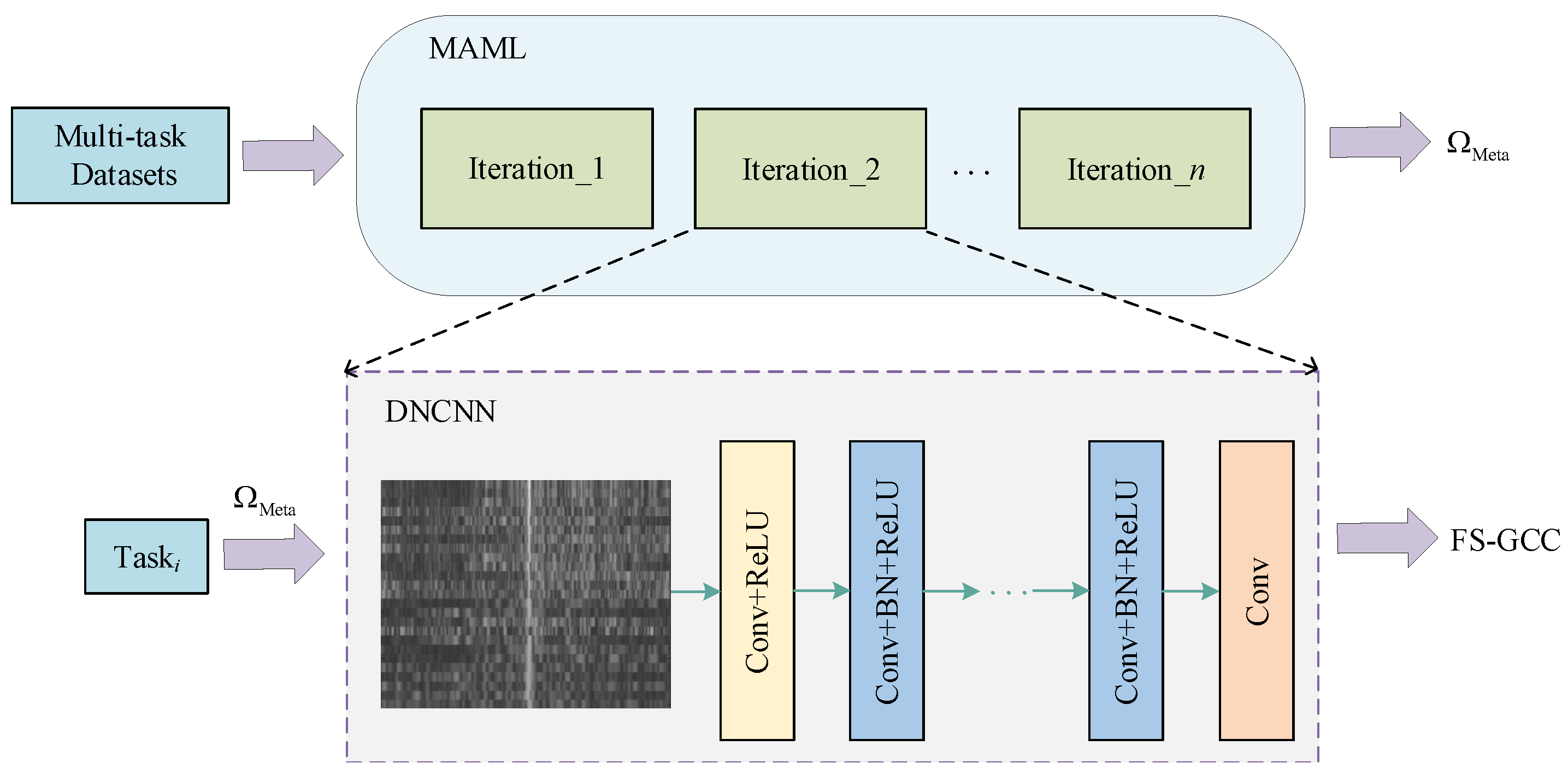
FS-GCC improves upon the GCC method, enabling the analysis of how various frequency bands contribute to the TDE of direct path. The size of the spectral window is $B$, and the hop length is $M$. $B$ and $M$ should be selected based on channel and signal characteristics. The subband GCC for any frequency band $l$ is defined as

$$R\left[l,\tau \right]={\displaystyle \frac{1}{2\pi }}{\int }_{-\pi }^{\pi }\mathrm{\Psi }(\omega +{\omega }_l)\mathrm{\Phi }\left(\omega \right)e^{j\omega \tau }d\omega$$

(10)

where $\mathrm{\Psi }\left(\omega \right)=G\left(\omega \right)\psi \left(\omega \right)$, ${\omega }_l$ represents the frequency offset of the subband $l$. $\mathrm{\Phi }\left(\omega \right)\in R$ is a symmetric frequency domain window centered at $\omega =0$ with a bandwidth of $B_{\mathrm{\Phi }}\in [0,\pi ]$.

The frequency-swept subband GCC can be obtained by scanning $\angle P\left(\omega \right)$ (cross-power spectrum phase) over potentially overlapping frequency bands:

$${\omega }_l=l{M}_{\mathrm{\Phi }}, l=0,\dots ,L-1$$

(11)

where $M_{\mathrm{\Phi }}$ is frequency hopping.

When selecting the number of subbands $L$, it must cover all frequencies and not exceed the Nyquist limit:

$$L=\left[{\displaystyle \frac{(\pi -B_0+M_{\mathrm{\Phi }})}{M_{\mathrm{\Phi }}}}\right]$$

(12)

In practical applications, we consider using the discrete Fourier transform (DFT) of underwater LFM signals to extract subband GCC. The DFT of underwater LFM signals $x_m\left[n\right]$ is represented as

$$X_m={\left[X_m\left[0\right],X_m\left[1\right],\dots ,0,0,\dots ,X_m\left[N-1\right]\right]}^T,m=1,2$$

(13)

where the elements $X_m\in C^N$ are the coefficients $X_m\left[k\right]$ of discrete frequencies ${\omega }_k=k{\displaystyle \frac{2\pi }{N}}$, and $n$ is DFT’s length. It includes the discrete frequency sample $\mathrm{\Phi }\left[k\right]=\mathrm{\Phi }\left({\omega }_k\right)$ symmetric frequency domain window vector $\mathrm{\Phi }$, represented as

$$\mathrm{\Phi }={\left[\mathrm{\Phi }\left[0\right],\mathrm{\Phi }\left[1\right],\dots ,0,0,\dots ,\mathrm{\Phi }\left[N-1\right]\right]}^T$$

(14)

where $\mathrm{\Phi }\in R^N$ performs symmetric zero-padding on $\mathrm{\Phi }$ to ensure it contains only $B=\left[2B_{\mathrm{\Phi }}{\displaystyle \frac{N}{2\pi }}\right]$ non-zero elements.

The subband GCC vector $r_l\in C^N$ is obtained through the inverse transform of the windowed PHAT spectrum DFT, represented as

$$r_l\left[n\right]={\displaystyle \frac{1}{N}}\sum _{k=0}^{N-1}{\displaystyle \frac{X_1\left[k+lM\right]X_2^{*}\left[k+lM\right]}{|X_1\left[k+lM\right]X_2^{*}\left[k+lM\right]}}\mathrm{\Phi }\left[k\right]e^{j{\displaystyle \frac{2\pi }{N}}kn}$$

(15)

where $M=\left[M_{\mathrm{\Phi }}{\displaystyle \frac{N}{2\pi }}\right]$ for discrete frequency hopping.

The FSGCC matrix is constructed by stacking subband GCC vectors together:

$$R=\left[r_0,r_1,\cdots ,r_{L-1}\right]\in C^{L\times N}$$

(16)

In the absence of noise, the true TDOA is located at the maximum value of each row $R\left[l,\tau \right]$. However, the presence of noise and reverberation affects the FS-GCC, making TDE more challenging. Figure 2 shows examples of FS-GCC for underwater LFM signals at different SNRs.

3. Proposed Method

In this section, our proposed method specifically includes two key steps:

• FS-GCC matrix Feature Enhancement: This step focuses on reconstructing multiple subwindow groups of the FS-GCC matrix to capture time delay-related signal features from various frequency band perspectives, enriching the information dimension and strengthening the key feature vectors.
• MAML-based DnCNN Network Optimization Training: The FS-GCC matrix is first converted into a grayscale image, and DnCNN’s multi-layer convolution is applied to automatically learn and extract the time delay features reconstructed from the FS-GCC, effectively suppressing noise interference. Then, we incorporate the MAML framework to facilitate training under various SNR conditions. This integration allows the model to rapidly adapt to new environments and learn efficiently with a limited number of samples, thereby improving its generalization capabilities and robustness across different SNR scenarios.

3.1. FS-GCC Matrix Feature Enhancement

According to reference [19], we designed a group of spectral windows ${\mathrm{\Phi }}_{group}=\left\{{\mathrm{\Phi }}_1,{\mathrm{\Phi }}_2,{\mathrm{\Phi }}_3,\dots ,{\mathrm{\Phi }}_N\right\}$ with a length of $N$. Then, the FS-GCC is computed for each window function ${\mathrm{\Phi }}_i(i\in \left\{1,2,\dots ,N\right\})$ in the window group ${\mathrm{\Phi }}_{group}$. The spectral window size $B$ and the spectral window hop length $M$ are defined as $B_{group}=\left\{B_{1,\mathrm{\Phi }},B_{2,\mathrm{\Phi }},B_{3,\mathrm{\Phi }},\dots ,B_{N,\mathrm{\Phi }}\right\}$ and $M_{group}=\left\{M_{1,\mathrm{\Phi }},M_{2,\mathrm{\Phi }},M_{3,\mathrm{\Phi }},\dots ,M_{N,\mathrm{\Phi }}\right\}$, respectively. Across the full frequency range, the window ${\mathrm{\Phi }}_i$ is slid to partition the cross-power spectrum phase into $L_i$ subbands. The FS-GCC for the $i$-th window ${\mathrm{\Phi }}_i$ is defined as follows:

$$R_i(l,\tau )={\displaystyle \frac{1}{2\pi }}{\int }_{-\pi }^{\pi }\mathrm{\Psi }(\omega +{\omega }_{i,l}){\mathrm{\Phi }}_i\left(\omega \right)e^{j\omega \tau }d\omega$$

(17)

where the frequency offset ${\omega }_{i,l}$ corresponds to the window $i$ and frequency band $l$. In the following expressions, $R_i(l,\tau )$, $\tau \in \left\{0,1,\dots ,N_t-1\right\}$ is represented as $R_{i,l}$.

Figure 3 shows a schematic diagram of two spectral windows sliding across the frequency domain, with $\angle (·)$ representing the complex-valued phase angle. The subband GCC can be interpreted as the product of the shifts of $\phi \left(\omega \right)$ and $\mathrm{\Phi }\left(\omega \right)$ to ${\omega }_l$, with the frequency shifted back to zero before performing the inverse Fourier transform.

Sliding each window ${\mathrm{\Phi }}_i$ from ${\mathrm{\Phi }}_{group}$ across the GCC frequency domain will produce $N$ subband matrices $R_i=\left[R_{i,0},R_{i,1},\cdots ,R_{i,L_{i-1}}\right]\in C^{L_i\times N_t}$, as shown in Figure 4a. Given that the dimensions of $R_i$ depend on the values of $B$ and $M$, it is necessary to standardize the dimensions for the subsequent CNN training. Additionally, the time delay information encoded in the FS-GCC matrices from different spectral windows exhibits distinct characteristics. Effectively integrating this information can improve the feature representation of the FS-GCC matrices. Therefore, to reconstruct $N$ FS-GCC matrices from multiple windows, the $N$ subband matrices are concatenated into a joint matrix $R_{joint}=\left[R_1,R_2,\dots ,R_N\right]$, as shown in Figure 4b. Let $m_{i,l}$ be the maximum value in each row of the matrix $R_{joint}$. By sorting $R_{joint}$ in descending order based on $m_{i,l}$, we obtain $R_{sort}=\left[R_{1_{-}sort},R_{2_{-}sort},\cdots ,R_{{\sum }_{i=1}^N{L}_{i-1-}sort}\right]$. The top $R_{L_{i-1}}$ rows are then retained to form the reconstructed FS-GCC matrix $R_{reco}=\left[R_{1_{-}sort},R_{2_{-}sort},\dots ,R_{L_{i-1_{-}}sort}\right]$. Sorting rows by their maximum values $m_{i,l}$ prioritizes subbands with the most prominent time delay peaks, which statistically correspond to less noise-corrupted components. The selection step then constructs a compact representation by retaining these optimal subbands, directly improving DnCNN’s input quality. As shown in Figure 4c, it can be observed that the time delay information in the reconstructed FS-GCC matrix is significantly enhanced.

3.2. Meta-DnCNN Network Optimization Training

3.2.1. MAML Framework

MAML is a meta-learning method based on initializing parameters. Its core concept revolves around refining the model’s initialization parameters through training across a spectrum of related tasks. This approach allows the training of new tasks to build upon prior training and adjustments, significantly improving the model’s training efficiency and convergence speed. Rather than modifying the neural network’s structure, MAML primarily focuses on optimizing and tuning the initialization parameters, which substantially mitigates the computational burden. From the perspective of the loss function, the learning process of MAML can be interpreted as maximizing the sensitivity of the new task’s loss function to the model parameters. It means that small parameter adjustments can significantly affect the task loss. MAML’s training strategy employs an inner and outer parameter update mechanism, as shown in Figure 5. The inner update in MAML addresses each task within the batch individually: each task is fed into the network, with the outer parameters serving as the foundation for initializing the inner parameters. The network weights are updated using the support set, and the task loss is evaluated through the query set. The outer update of MAML is based on the performance of all tasks within the batch: the losses of all subtasks are summed, and this sum is used to update the outer parameters of the network. The advantage of this strategy is that it ensures consistency between local training tasks and test tasks while also expanding the training data distribution, thereby improving the model’s generalization ability.

The mathematical framework of the MAML algorithm is as follows: Suppose we have a neural network model $f_{\theta }$ initialized with parameter $\theta$, and the training task distribution is denoted as $p\left(\mathcal{T}\right)$. When performing inner-loop parameter ${\theta }_i^{\prime }$ updates for task ${\mathcal{T}}_i$, we can use the following formula:

$${\theta }_i^{\prime }=\theta -\alpha {\nabla }_{\theta }{\mathcal{L}}_{{\mathcal{T}}_i}\left(f_{\theta }\right)$$

(18)

where $\alpha$ is the inner-loop learning rate, which represents the step size of gradient descent. To ensure that the network performs well on all tasks in the current batch, we update the network parameters by summing the losses of all tasks to form a batch loss and minimizing this loss. The formula for outer-loop parameter updates is as follows:

$$\theta \leftarrow \theta -\beta {\nabla }_{\theta }\sum _{{\mathcal{T}}_i\sim p\left(\mathcal{T}\right)}{\mathcal{L}}_{{\mathcal{T}}_i}\left(f_{{\theta }_i^{\prime }}\right)$$

(19)

where $\beta$ is the learning rate for outer-loop updates. It is worth noting that although the loss $L$ is computed using ${\theta }_i^{\prime }$ in the formula, the subsequent updates are not made to ${\theta }_i^{\prime }$ but rather to $\theta$, which are the initialization parameters for the outer loop. Algorithm 1 outlines the Training Stage of MAML.

Algorithm 1 The training stage of MAML

Input:  Set of tasks $\mathcal{T}=\left\{{\mathcal{T}}_1,{\mathcal{T}}_2,\dots ,{\mathcal{T}}_n\right\}$, $\alpha$, $\beta$ Output:  $\theta$  1: Initialize $\theta$ of the model $f_{\theta }$  2: while not done do  3:    for each ${\mathcal{T}}_i\in {\mathcal{T}}_i\sim p\left(\mathcal{T}\right)$ do  4:      Initialize the network with $\theta$  5:      Gradient descent using $\alpha$  6:      Obtain ${\theta }_i^{\prime }$ according to Equation (18)  7:    end for  8:    Gradient descent using $\beta$  9:    Update $\theta$ according to Equation (19) 10: end while 11: return  $\theta$

3.2.2. Meta-DnCNN Model

In this paper, we apply the MAML training strategy to the DnCNN model, naming it Meta-DnCNN. The objective is to leverage meta-learning to enhance the model’s adaptability and robustness across various SNR environments. Even with a limited training dataset, the model effectively suppresses noise interference and extracts delay features from the FS-GCC matrix, significantly reducing the network’s reliance on large-scale training data. The specific implementation steps are illustrated in Figure 6. We convert FS-GCC matrix data obtained under different SNR conditions into grayscale images to construct multi-task datasets, which are then fed into the MAML model. With DnCNN serving as the base model for MAML, continuous iterations through the MAML training strategy ${\mathrm{\Omega }}_{Meta}$ ultimately yield the predicted FS-GCC matrix.

DnCNN Model:

The DnCNN model is designed based on the deep neural network architecture of the VGG (Visual Geometry Group), which utilizes repeated convolutional blocks [25]. Typically, deep learning-based methods aim to establish a mapping from noisy images to denoised images. However, unlike other deep learning-based denoising algorithms, the DnCNN model employs residual learning, where the network focuses on learning the noise characteristics rather than the image features. It predicts the noise component, and the denoised image is then obtained by subtracting the predicted noise component from the noisy image. The model’s principle is illustrated in the lower part of Figure 6.

During the training process, the DnCNN model’s output is the predicted residual image, and the target output is the difference between the noisy and noise-free images. The difference between these two images serves as the loss function for error backpropagation, which adjusts the network parameters. In the DnCNN model, the Mean Square Error (MSE) is used as the loss function, with the specific expression shown in Equation (20):

$$l\left(\theta \right)={\displaystyle \frac{1}{2N}}\sum _{i=1}^N\left|\right|R(y_i,\theta )-(y_i-x_i){\left|\right|}^2$$

(20)

where $R(y_i,\theta )$ represents the predicted residual output, $y_i$ and $x_i$ denote the noisy and noise-free images, respectively, $N$ is the number of samples, and $\theta$ refers to the network parameters.

In this paper, the DnCNN network model consists of 13 layers. The first layer combines convolution with the ReLU function. The middle layers consist of convolution, BN (Batch Normalization), and ReLU functions to accelerate convergence. The model ends with a convolutional layer. The convolutional kernels are of size 3 × 3, with both stride and padding set to 1.

MAML Training Process:

Step 1. Dataset Construction: Since the inner loop of the MAML algorithm is designed for datasets with consistent distributions, the experimental data consists of grayscale images derived from FS-GCC matrices under varying SNR conditions. These images serve as the MAML training tasks for the experimental model. The grayscale images $F_p$ generated from noisy FS-GCC matrices are used as inputs for DnCNN, while the corresponding grayscale images $F$ derived from noise-free FS-GCC matrices function as the target labels. The task set for MAML can be expressed as

$$\mathcal{T}=\left\{{(F_p,F)}_1,{(F_p,F)}_2,\dots ,{(F_p,F)}_n\right\}$$

(21)

Within each task, the dataset is further divided into support sets ${\mathrm{\Psi }}_i^{sup}={(F_p,F)}_i$ and query sets ${\mathrm{\Xi }}_i^{que}={(F_p,F)}_i$, which are analogous to training and test sets in traditional deep learning model. These sets are mutually exclusive.

Step 2. MAML Training Process: After constructing the task sets, MAML trains separately through the inner-loop learner and the outer-loop meta-learner. The inner-loop learner uses sample data from the support sets ${\mathrm{\Psi }}_i^{sup}={(F_p,F)}_i$ for training, as described in Equation (18). The outer-loop learner iterates over sample data from the query sets ${\mathrm{\Xi }}_i^{que}={(F_p,F)}_i$ across different tasks based on Equation (19). By learning across multiple tasks, the model is able to acquire an initialization parameter that is suitable for all tasks, thereby enabling the model to “learn to learn". This ability allows the model to rapidly converge and adjust parameters when encountering new tasks, achieving fast learning.

Step 3. Fine-Tuning Process: After completing MAML training, the model is equipped with a set of initialization parameters. When faced with a new task, the parameters can be further adjusted through fine-tuning based on these initialization parameters. This adjustment leads to faster convergence and requires fewer samples. First, a new task dataset ${\mathcal{T}}_{new}=\left\{{(F_p,F)}_1,{(F_p,F)}_2,\dots ,{(F_p,F)}_n\right\}$ is constructed, and the support set data ${\mathrm{\Psi }}_{new}^{sup}={(F_p,F)}_i$ are used to update the model’s parameters. A relatively small number of samples is sufficient to obtain an optimized Meta-DnCNN model that better adapts to the data distribution of the new task.

Step 4. MAML Testing Process: Following training and fine-tuning, the DnCNN model is saved and employed for FS-GCC estimation in new SNR environments. Its performance is evaluated by comparing the results with grayscale images of FS-GCC matrices under noise-free conditions. This comparison assesses the generalization performance of the proposed algorithm in unfamiliar environments, validating the model’s adaptability and accuracy in practical applications across a range of SNR conditions.

4. Simulation Results and Discussion

This section exhibits the simulation results, verifies the effectiveness of the proposed method, and discusses the results accordingly.

4.1. Evaluation Metrics

To assess the effectiveness of TDE, the following metrics are used: mean absolute error (MAE), percentage of abnormal points (PAP), and FSPR.

MAE is a metric that quantifies the average absolute difference between estimated delays and actual delays. It serves as a measure of the overall accuracy of an algorithm in estimating delay values. The MAE is calculated using the following formula:

$$MAE={\displaystyle \frac{1}{N_{total}}}\sum _{i=1}^{N_{tial}}|D_i-D|,$$

(22)

where $D$ is the true value of the time delay, $D_i$ is the TDE for the $i$-th test, $N_{total}$ represents the total estimated samples.

PAP represents the ratio of abnormal estimated samples to the total estimated samples. This metric helps to detect significant discrepancies or errors in the TDE process. It is computed using the following formulas:

$$PAP={\displaystyle \frac{N_n}{N_{total}}}$$

(23)

where $N_n$ represents the set of abnormal estimated samples. A TDE error exceeding 5 sampling points is considered an abnormal estimation result.

FSPR is described as the mean increase of the highest GCC peak compared with the second highest peak.

$$FSPR={\displaystyle \frac{1}{N_{total}}}\sum _{i=1}^{N_{total}}20log10\left({\displaystyle \frac{p_1^i}{p_2^i}}\right)$$

(24)

where $p_1^i$ and $p_2^i$ represent the highest and second highest peak values, respectively.

4.2. Simulation Settings

We consider LFM signals with center frequency is $11$ kHz, sampling rate is 50 kHz, B = 8 kHz and $T=0.01$ s for TDE as shown in Figure 1. The underwater channel environment is intercepted from the NOF and NCS channel of the Watermark underwater channel dataset [26]. The intercepted NOF and NCS channel impulse response in this experiment is shown in Figure 7a,b.

We defined a frequency window group ${\mathrm{\Phi }}_{group}$, where $B_{group}=\left\{32,64,128,256\right\}$ and $M_{group}=\left\{B_{group}/8\right\}$ are the coefficients of spectrum window function. We added white Gaussian noise to the received signal, where the SNR ranges from −20 dB to 10 dB, incrementing by 5 dB each time. Furthermore, 200 Monte Carlo simulations are conducted for each SNR level. The parameters of the eta-DnCNN network are outlined in

Table 1. Network simulation parameters of Meta-DnCNN.

Parameters	Value
Number of Tasks	6
SNR of Training Tasks	−15∼10 dB
Number of Training Data of Each Task	150
Number of Test Data of Each Task	20
Outer-Loop Learning Rate	0.001
Inner-Loop Learning Rate	0.001
Epoch	200
Optimizer	Adam

, noting that the training task’s SNR is varied in steps of 5 dB.

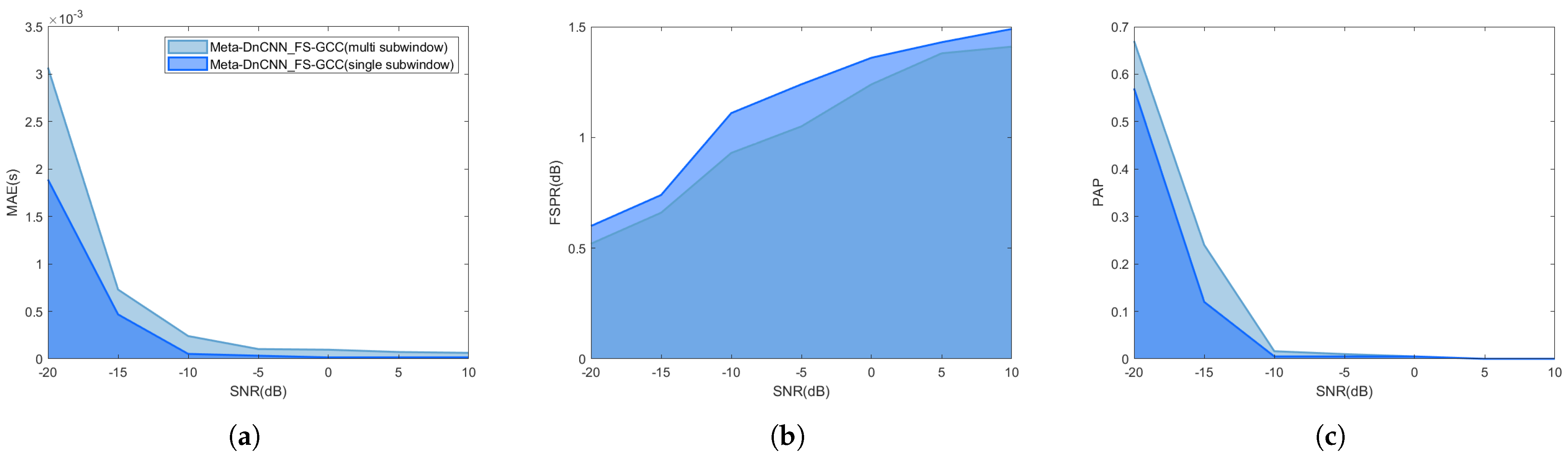
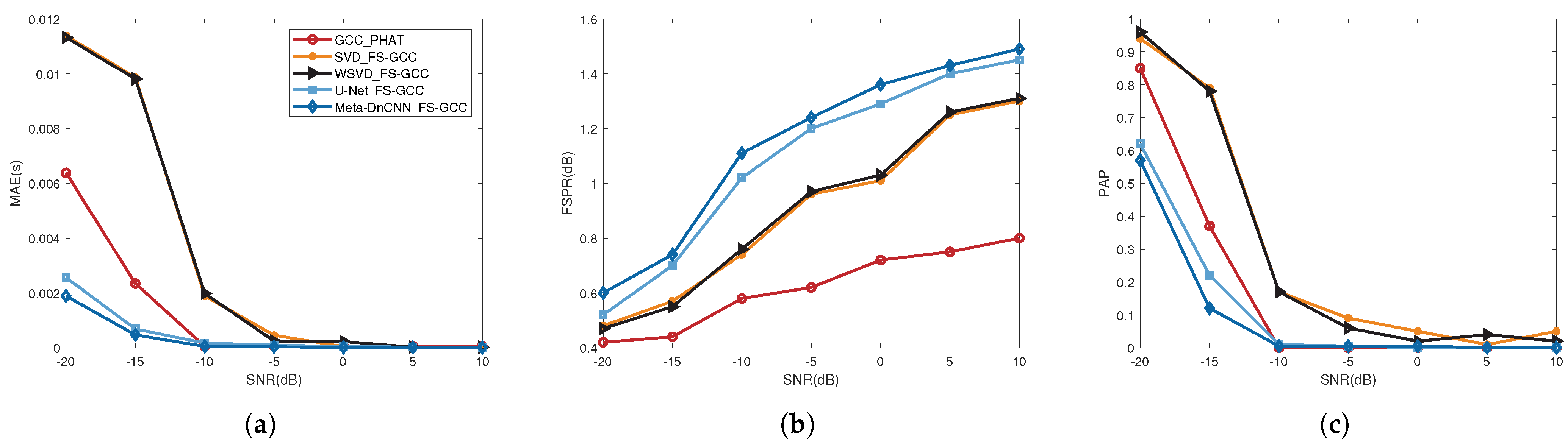
4.3. TDE Results and Analysis

Figure 8 displays the single prediction results of our proposed method for FS-GCC under NOF channel when SNR is −10 dB. Specifically, Figure 8a depicts the original FS-GCC matrix, Figure 8b shows the FS-GCC matrix under noise-free conditions, and Figure 8c presents the predicted FS-GCC matrix. Notably, Figure 8c is the restored FS-GCC matrix obtained from the gray image predicted by the Meta-DnCNN network. It is evident that Meta-DnCNN method effectively recovers the time delay characteristics of the FS-GCC matrix under noise-free conditions.

Figure 9a–d show the peaks of single TDE results of GCC_PHAT, SVD_FS-GCC [18], WSVD_FS-GCC [18], and Meta-DnCNN_FS-GCC, respectively, where the red line indicates the sampling point values of the correct TDE. As can be observed, the peak value of the traditional GCC_PHAT method is not prominent in high SNR underwater channel environments, which tends to result in a high anomaly rate in predictions. Both the SVD_FS-GCC and WSVD_FS-GCC methods effectively mitigate the impact of clutter peaks. However, the proposed method further enhances the peaks and exhibits greater stability during the prediction process.

Figure 10 and Figure 11 show the TDE performance of the Meta-DnCNN_FS-GCC method with single subwindow and multi-sub-window reconstruction for white Gaussian noise with different SNR added for NOF and NCS channels, respectively. The single subwindow we chosen is the frequency window with $B=256$ and $M=32$. It can be observed that the Meta-DnCNN_FS-GCC method using multi-sub-window reconstruction outperforms the single subwindow method across all performance indicators. This improvement is attributed to the multi-sub-window reconstruction operation, which enhances the characteristics of the FS-GCC matrix, leading to a more pronounced peak in the cross-correlation estimation and thereby increasing both the accuracy and stability of the estimation. This finding is consistent in both channel environments, although the NCS channel, being more complex than the NOF channel, exhibits slightly worse performance metrics.

Figure 12 and Figure 13 present the MAE, FSPR, and PAP of NOF and NCS channels for the GCC_PHAT, SVD_FS-GCC [18], WSVD_FS-GCC [18], U−Net_FS-GCC [20], and Meta-DnCNN_FS-GCC methods with the addition of Gaussian white noise with different SNR, respectively. The U-Net network in reference [20] was also trained using MAML. As shown in Figure 12a and Figure 13a, the MAE of TDE decreases with an increase in SNR. Under low SNR conditions, the MAE of the deep learning-based methods shows significant improvement compared with existing methods, with the Meta-DnCNN_FS-GCC method further enhancing TDE accuracy relative to the U−Net_FS-GCC method. Figure 12b and Figure 13b illustrate the variation in FSPR under different SNR conditions. A higher FSPR corresponds to a more pronounced peak. The traditional GCC method exhibits weak peaks at low SNR, while methods based on SVD and deep learning demonstrate superior peak significance. The Meta-DnCNN_FS-GCC method further accentuates the peak by enhancing the FS-GCC matrix characteristics. Figure 12c and Figure 13c show the variation in PAP with SNR. As the SNR decreases, the probability of TDE anomalies increases. However, the Meta-DnCNN_FS-GCC method maintains stability and effectively mitigates the occurrence of such abnormal estimations.

5. Discussion

This paper analyses the performance of the Meta-DnCNN_FS-GCC method through a series of experiments. The results clearly demonstrate that in the complex and variable underwater channel environment, especially under the condition of low SNRs, the Meta-DnCNN_FS-GCC method shows significant advantages, with the MAE reduced, the FSPR higher, and the PAP effectively controlled.

The peak of the traditional GCC_PHAT method is not obvious, which is consistent with the conclusion in the existing literature that its ability to capture signal features in a complex channel environment is limited. Based on the cross-correlation principle, GCC_PHAT performs well under ideal conditions but is severely impacted by multi-path propagation and noise interference in underwater environments. As noted in reference [17], when numerous reflections and noise are present in the channel, GCC_PHAT struggles to accurately differentiate the true time delay peak from false peaks induced by interference signals. This leads to a high anomaly rate and high estimation errors. In contrast, the SVD_FS-GCC and WSVD_FS-GCC methods, which incorporate singular-value decomposition to process the FS-GCC matrix, are more effective in suppressing clutter peaks. By decomposing the signal matrix into a subspace containing the primary signal features and a noise subspace, these methods reduce noise components, making the time delay peak more obvious. This result is consistent with the conclusion about the noise reduction and feature enhancement of singular-value decomposition in signal processing proposed in reference [18]. However, the SVD method is easily affected by spurious peaks, so the accuracy and stability of TDE are not ideal in underwater channels.

Under low SNRs, some frequency bands of the signal can be severely polluted by noise, making it difficult for traditional methods to extract effective time delay information. The multi-sub-window reconstruction can capture the time delay features from different frequency bands, and each subwindow can be regarded as an analysis window of the signal in a specific frequency range. In this way, even if some frequency bands are strongly interfered by noise, other frequency bands may still capture relatively clear time delay features, thus avoiding the overall estimation anomaly caused by the loss of partial frequency band information. It can be seen from Figure 4 that this method of comprehensively extracting features from multiple frequency bands enriches the information dimension of the FS-GCC matrix and enhances its key eigenvectors. Our experiments confirm that this approach facilitates comprehensive TDE even under low SNR conditions, providing more basis for subsequent accurate estimation and reducing the probability of abnormal estimation. This is consistent with the conclusion about the advantage of multi-band signal processing in capturing the key features of time delay in reference [19]. On this basis, the Meta-DnCNN_FS-GCC method proposed in this paper further highlights the peak. By leveraging the denoising and feature extraction capabilities of DnCNN, the method transforms the FS-GCC matrix into a grayscale image and applies a multi-layer convolutional network to automatically learn noise features. This enables more accurate extraction of useful time delay information from noisy signals and restores the FS-GCC matrix closer to a noise-free state. As a result, time delay estimation remains stable even under high SNR, reducing prediction anomalies. Additionally, the application of the MAML framework enables the model to obtain good performance with only 150 pieces of data in each group of tasks. When facing a new task with a SNR of −20 dB, the model can quickly adjust its parameters based on the feature extraction methods and noise suppression strategies learned under various SNR conditions before, allowing for accurate TDE despite limited data. This knowledge-sharing capability significantly enhances the model’s practicality and robustness in dynamic underwater environments.

However, there are still some areas for improvement in the method of this study. For example, although the Meta-DnCNN_FS-GCC performs excellently under the current experimental settings, the complexity of the actual underwater environment may exceed the scope of experimental simulation. Future research can further explore how to further optimize and improve the TDE under more extreme underwater environmental conditions, such as strong water currents and severe multi-path effects caused by complex geological structures, so as to meet the needs of the continuous development of underwater engineering and scientific research.

6. Conclusions

Aiming at the challenges of accuracy and stability in time delay estimation under low SNRs in underwater signal processing, as well as the problem that the existing methods based on cross-correlation and deep learning fail to meet the practical application requirements, this paper proposes an innovative solution that combines a multi-sub-window reconstruction of the FS-GCC matrix, multi-layer convolution denoising of the DnCNN, and the MAML framework. Through multi-sub-window reconstruction, this solution captures and enhances the extraction of time delay characteristics from different frequency bands. The DnCNN is utilized to accurately extract multi-level noise features for noise suppression. With the help of the MAML, the model can quickly adapt to new environments under various SNR conditions. Even with a limited number of underwater training samples, it can achieve the desired accuracy, significantly improving the accuracy and stability of underwater time delay estimation, as well as the practicability and robustness of the model in complex underwater environments. We conducted simulation experiments in a real underwater acoustic channel environment. By analyzing the experimental results, we explored the limitations of the existing methods and investigated the advantages of the proposed method in underwater time delay estimation. The experimental results show that, compared with the existing methods, the proposed method reduces the MAE, increases the FSPR, and effectively controls the PAP. Under the same conditions, it has lower estimation errors and higher stability. This innovation provides strong support for the efficient and stable operation of underwater sensor networks and also offers new ideas for applying the human voice time delay estimation methods to the underwater environment.

References

1. Luo, J.; Yang, Y.; Wang, Z.; Chen, Y. Localization algorithm for underwater sensor network: A review. IEEE Internet Things J. 2021, 8, 13126–13144. [Google Scholar] [CrossRef]
2. Li, S.; Qu, W.; Liu, C.; Qiu, T.; Zhao, Z. Survey on high reliability wireless communication for underwater sensor networks. J. Netw. Comput. Appl. 2019, 148, 102446. [Google Scholar] [CrossRef]
3. Fan, H.; Nie, W.; Yao, S.; An, L.; Yu, F.; Zhang, Y.; Wu, Q. A high-order time-delay difference estimation method for signal enhancement in the distorted towed hydrophone array. J. Acoust. Soc. Am. 2024, 156, 1996–2008. [Google Scholar] [CrossRef]
4. Wang, X.; Xu, B.; Guo, Y. Minimum error entropy robust delay filter for multi-auv cooperative localization. IEEE/ASME Trans. Mechatronics 2024, 30, 1567–1577. [Google Scholar] [CrossRef]
5. Xia, Z.; Li, X.; Meng, X. High resolution time-delay estimation of underwater target geometric scattering. Appl. Acoust. 2016, 114, 111–117. [Google Scholar] [CrossRef]
6. Lowes, G.J.; Neasham, J. PADAL—Passive acoustic detection and localisation: Low energy underwater wireless vessel tracking network. Comput. Netw. 2024, 241, 110216. [Google Scholar] [CrossRef]
7. Jo, M.J.; Choi, J.W.; Han, D.G. Estimation of Source Range and Location Using Ship-Radiated Noise Measured by Two Vertical Line Arrays with a Feed-Forward Neural Network. J. Mar. Sci. Eng. 2024, 12, 1665. [Google Scholar] [CrossRef]
8. Hu, X.; Zhang, L.; Hu, B.; Wang, J.; Guo, L.; Zhang, H. Position estimation of acoustic elements based on improved delay estimation algorithm. Appl. Acoust. 2025, 228, 110286. [Google Scholar] [CrossRef]
9. Jang, J.; Meyer, F.; Snyder, E.R.; Wiggins, S.M.; Baumann-Pickering, S.; Hildebrand, J.A. Bayesian detection and tracking of odontocetes in 3-D from their echolocation clicks. J. Acoust. Soc. Am. 2023, 153, 2690. [Google Scholar] [CrossRef]
10. Jia, L.; Zhang, G.; Liu, Y.; Bai, Z.; Geng, Y.; Wu, Y.; Zhang, J.; Zhang, W. Sonar buoy active detection and localization for underwater targets using high-level sound sources and MEMS hydrophone. Measurement 2025, 241, 115740. [Google Scholar] [CrossRef]
11. Pang, X.; Jiang, F. Generalized quadratic correlation delay estimation algorithm based on Phase Transform weighting function. In Proceedings of the 2023 7th International Conference on Electronic Information Technology and Computer Engineering, Xiamen, China, 20–22 October 2023; pp. 1069–1074. [Google Scholar]
12. Ferguson, E.L. Multitask convolutional neural network for acoustic localization of a transiting broadband source using a hydrophone array. J. Acoust. Soc. Am. 2021, 150, 248–256. [Google Scholar] [CrossRef]
13. Whitaker, S.; Barnard, A.; Anderson, G.D.; Havens, T.C. Through-ice acoustic source tracking using vision transformers with ordinal classification. Sensors 2022, 22, 4703. [Google Scholar] [CrossRef]
14. Yao, S.; Meng, Q.; Chen, C.; Tariq, I.; Zhou, C.; Liu, W. High-precision time delay estimation of narrowband radio signal by PHAT-LSTM. Meas. Sci. Technol. 2021, 32, 075001. [Google Scholar] [CrossRef]
15. Salvati, D.; Drioli, C.; Foresti, G.L. Time delay estimation for speaker localization using CNN-based parametrized GCC-PHAT features. In Proceedings of the Interspeech, Brno, Czechia, 30 August–3 September 2021; pp. 1479–1483. [Google Scholar]
16. Comanducci, L.; Borra, F.; Bestagini, P.; Antonacci, F.; Tubaro, S.; Sarti, A. Source localization using distributed microphones in reverberant environments based on deep learning and ray space transform. IEEE/ACM Trans. Audio Speech Lang Process. 2020, 28, 2238–2251. [Google Scholar] [CrossRef]
17. Wang, S.; Zhou, Y.; Yang, X.; Liu, H. A robust blind source separation algorithm based on non-negative matrix factorization and frequency-sliding generalized cross-correlation. In Proceedings of the 2021 IEEE Statistical Signal Processing Workshop (SSP), Rio de Janeiro, Brazil, 11–14 July 2021; pp. 231–235. [Google Scholar]
18. Cobos, M.; Antonacci, F.; Comanducci, L.; Sarti, A. Frequency-sliding generalized cross-correlation: A sub-band time delay estimation approach. IEEE/ACM Trans. Audio Speech Lang. Process. 2020, 28, 1270–1281. [Google Scholar] [CrossRef]
19. Song, Q.; Ou, Z. Modified frequency-sliding generalized cross correlation for time delay difference estimation of microphone array. IEEE Sensors J. 2023, 23, 31038–31049. [Google Scholar] [CrossRef]
20. Comanducci, L.; Cobos, M.; Antonacci, F.; Sarti, A. Time difference of arrival estimation from frequency-sliding generalized cross-correlations using convolutional neural networks. In Proceedings of the ICASSP 2020-2020 IEEE International Conference on Acoustics, Speech and Signal Processing (ICASSP), Barcelona, Spain, 4–8 May 2020; pp. 4945–4949. [Google Scholar]
21. Yang, N.; Zhang, B.; Ding, G.; Wei, Y.; Wei, G.; Wang, J.; Guo, D. Specific emitter identification with limited samples: A model-agnostic meta-learning approach. IEEE Commun. Lett. 2021, 26, 345–349. [Google Scholar] [CrossRef]
22. Lin, W.; Mak, M.W. Model-agnostic meta-learning for fast text-dependent speaker embedding adaptation. IEEE/ACM Trans. Audio Speech Lang. Process. 2023, 31, 1866–1876. [Google Scholar] [CrossRef]
23. Yang, F.; Liu, J.; Hua, C.; Liu, W.; Dong, D. Early fault diagnosis strategy for high-speed train suspension systems based on model-agnostic meta-learning. Veh. Syst. Dyn. 2024, 62, 2510–2532. [Google Scholar] [CrossRef]
24. Wu, J.; Li, M.; Fang, X.; Ramaccia, D.; Toscano, A.; Bilotti, F.; Ding, D. Anti-interference DoA estimation for LFM radar signals using space-time-modulated metasurfaces. IEEE Trans. Microw. Theory Tech. 2024, 73, 1460–1472. [Google Scholar] [CrossRef]
25. Mehdizadeh, M.; MacNish, C.; Xiao, D.; Alonso-Caneiro, D.; Kugelman, J.; Bennamoun, M. Deep feature loss to denoise OCT images using deep neural networks. J. Biomed. Opt. 2021, 26, 046003. [Google Scholar] [CrossRef] [PubMed]
26. Van Walree, P.A.; Socheleau, F.X.; Otnes, R.; Jenserud, T. The watermark benchmark for underwater acoustic modulation schemes. IEEE J. Ocean. Eng. 2017, 42, 1007–1018. [Google Scholar] [CrossRef]
Figure 1. Time-domain and frequency-domain of LFM signal: (a) Time-domain. (b) Frequency-domain.
Jmse 13 00919 g001
Figure 2. Examples of FS-GCC at different SNRs: (a) SNR = −10 dB. (b) SNR = 0 dB. (c) SNR = 10 dB.
Jmse 13 00919 g002
Figure 3. Explanation of different spectral windows in FS-GCC: (a) Spectral window 1. (b) Spectral window 2.
Jmse 13 00919 g003
Figure 4. Reconstruction process of multi-window FS-GCC matrix at SNR = −10 dB: (a) Subband matrices. (b) Jointed matrix. (c) Reconstructed matrix.
Jmse 13 00919 g004
Figure 5. The parameter update mechanism of MAML.
Jmse 13 00919 g005
Figure 6. The Meta-DnCNN model.
Jmse 13 00919 g006
Figure 7. Watermark channel impulse response: (a) NOF channel. (b) NCS channel.
Jmse 13 00919 g007
Figure 8. Single prediction results: (a) Original FS-GCC matrix. (b) FS-GCC matrix under noise-free conditions. (c) Predicted FS-GCC matrix.
Jmse 13 00919 g008
Figure 9. Single estimated peak comparison: (a) GCC_PHAT. (b) SVD_FS-GCC. (c) WSVD_FS-GCC. (d) Meta-DnCNN_FS-GCC.
Jmse 13 00919 g009
Figure 10. TDE performance for multi-window and single-window Meta-DnCNN_FS-GCC under NOF channel: (a) MAE. (b) FSPR. (c) PAP.
Jmse 13 00919 g010
Figure 11. TDE performance for multi-window and single-window Meta-DnCNN_FS-GCC under NCS channel: (a) MAE. (b) FSPR. (c) PAP.
Jmse 13 00919 g011
Figure 12. TDE performance for methods under NOF channel: (a) MAE. (b) FSPR. (c) PAP.
Jmse 13 00919 g012
Figure 13. TDE performance for methods under NCS channel: (a) MAE. (b) FSPR. (c) PAP.
Jmse 13 00919 g013