NSMO-Based Adaptive Finite-Time Command-Filtered Backstepping Speed Controller for New Energy Hybrid Ship PMSM Propulsion System

Abstract

In the context of the new energy hybrid ship propulsion system (NE-HSPS), the parameters of the rotor speed, torque, and current of the permanent magnet synchronous motor (PMSM) are susceptible to environmental variations and unmodeled disturbances. Conventional nonlinear controllers (e.g., backstepping, PI, and sliding mode) encounter challenges related to response speed, interference immunity, and vibration jitter. These challenges stem from the inherent uncertainties in perturbations and the limitations of the traditional nonlinear controllers. In this paper, a novel Adaptive Finite-Time Command-Filtered Backstepping Controller (AFTCFBC) is proposed, featuring a faster response time and the elimination of overshoot. The proposed controller is a significant advancement in the field, addressing the computational complexity of backstepping control and reducing the maximum steady-state error of the control output. The novel controller incorporates a Nonlinear Finite-Time Command Filter (NFTCF) adapted to the variation in motor speed. Secondly, a novel Nonlinear Sliding Mode Observer (NSMO) is proposed based on the designed nonlinear sliding mode gain function (φ(S_w)) to estimate the load disturbance of the electric propulsion system. The Uncertainty Parameter-Adaptive law (UPAL) is designed based on Lyapunov theory to improve the robust performance of the system. The construction of a simulation model of a hybrid ship PMSM under four distinct working conditions, including constant speed and constant torque, the lifting and lowering of speed, loading and unloading, and white noise interference, is presented. The results of this study demonstrate a significant reduction in speed-tracking overshoot to zero, a substantial decrease in integral squared error by 90.15%, and a notable improvement in response time by 18.6%.

1. Introduction

In light of the intensification of the global greenhouse effect, there has been a global consensus to actively respond to the dual-carbon development goal of low-carbon and zero-carbon fuels. In order to effectively reduce carbon emissions from the shipping sector, the International Maritime Organization (IMO) has introduced a series of laws and regulations. However, despite these measures, the global shipping industry is still facing tremendous pressure, and there is an urgent need for in-depth research and exploration of innovative solutions [1,2].

As a significant component of global trade, shipping has emerged as a crucial mode of transportation in transoceanic trade, offering substantial economic and regional advantages. Statistical data indicate that approximately 90% of global trade is dependent on maritime transportation, yet 3% of the total global carbon footprint is attributed to this sector [3]. In response to the issue of marine pollution and excessive carbon emissions resulting from fuel consumption, the advancement of novel energy hybrid (or all-electric) vessels, waste heat recovery, and other technologies has emerged as a pivotal research area, with the objective of enhancing the energy efficiency of ships [4]. These ships integrate environmentally friendly fuels, including methanol (Sinopharm Chemical Reagent Co. Ltd., Shanghai, China), ammonia (KBR, Houston, TX, USA), and methane–ammonia blends (MAN Energy Solutions, Hamburg, Germany), with novel energy sources, such as solar and wind, to create hybrid ship propulsion systems, representing a significant stride toward sustainable container shipping [5,6,7]. Nevertheless, the performance of the propulsion motor, which constitutes a pivotal element in the ship electric propulsion system, will inevitably influence the overall efficiency of the system. While the implementation of wind–light–electric–fuel hybrid propulsion systems allows for the comprehensive utilization of multiple energy sources, enhancing energy utilization efficiency [8], various propulsion motors still encounter significant challenges in the dynamic and evolving marine environment. These challenges include the fluctuating parameters of internal resistance and the friction coefficient, as well as external sea state-induced disturbances. These factors collectively impact the control performance of electric propulsion systems [9].

PMSMs are widely utilized in high-speed precision machinery, flywheel energy storage, aerospace, and shipboard transportation due to their simple structure, high torque density, superior efficiency, and good reliability. They have become the predominant propulsion motors for current hybrid ships [10,11]. However, their nonlinear and time-varying characteristics, as well as the coupling of motor parameters, make it challenging to measure disturbances in the control process, while the motor parameters also change over time [12]. To ensure the controllability and maneuverability of the ship during navigation, the control strategy of the motor drive must meet stricter requirements.

The present study examines the multi-branch fusion research architecture of the control algorithm of the PMSM drive system, which comprises four major categories: traditional control, intelligent control, robust control, and nonlinear control. The central problem that needs to be solved in this field is the construction of a controller with dynamic parameter-adaptive ability to improve the system’s anti-disturbance performance. The following analysis reviews the research progress of different control strategies: In the realm of traditional controllers, notable examples include classical Proportional–Integral Differentiation (PID) control and backstepping control, which are distinguished by their simplicity and ease of engineering implementation. In a recent study, Fadzrizan Mohd Hanif et al. [13] proposed a novel piecewise affine PI controller for a buck converter-generated DC motor. The proposed PA function is expected to provide better control accuracy. Zhang et al. [14] proposed an adaptive proportional–integral resonance controller to suppress inverter speed pulsation and improve the stability of the system at different speeds. Wang et al. [15] and Nguyen et al. [16] proposed a backstepping observer based on a backstepping control algorithm that estimates the inverse electromotive force and disturbances of the motor system, thereby reducing the system state error. In terms of the intelligent controller, the system’s ability to handle nonlinear disturbances is significantly improved by incorporating artificial intelligence techniques such as fuzzy inference and neural networks. In a recent research analysis, Subarao et al. [17] presented the design, control, and performance comparison of PI and ANFIS controllers for BLDC motor-driven electric vehicles and verified that the ANFIS controller exhibited superior dynamic performance. In another study, Kroics et al. [18] proposed a BLDC motor speed control with a digital adaptive PID–fuzzy controller and reduced the harmonic content to shorten the transition time and avoid the overshoot phenomenon. The authors of [19] proposed a PID control algorithm based on a multi-strategy enhanced dung beetle optimizer and back-propagation neural network for DC motor control, which was applied to improve the control accuracy of the DC motor system. Lotfi et al. [20] proposed a data-driven Brain Emotional Learning-Based Intelligent Controller (BELBIC) for nonlinear MIMO systems to study the control of nonlinear multiple-input multiple-output (MIMO) systems by dynamically adjusting the probability coefficients. Liu et al. [21], Wang et al. [22], and Yue et al. [23] used intelligent control strategies combining neural networks, deep learning, and data-driven methods, which were applied to improve the dynamic performance of Permanent Magnet Synchronous Motors (PMSMs) and optimize the regulation effect of controller parameters and power allocation. In the domain of robust controllers, sliding mode control (SMC) and the algorithms derived from it represent a fundamental framework, exhibiting distinct advantages in addressing uncertainties. The efficacy of these methods is further enhanced by the introduction of various observers, including the Sliding Mode Observer (SMO) [24], the Extended Sliding Mode Load Torque Observer with Variable Structure (ESMLTO) [25], the Learning Observer [26], the Hyper-Twisted Observer [27], etc., which enable the controller to be effectively applied to situations with variable system parameters and complex perturbations. For example, Chen et al. [28] designed a robust model-free ultra-twisted sliding mode control method based on the Extended Sliding Mode Disturbance Observer (ESMDO) for improving the anti-interference capability of motor systems. Tian et al. [29] proposed a robust adaptive resonance control method, which is applied to the problem of poor robustness of adaptive resonance control in the face of non-periodic disturbances, and Wang et al. [30] proposed a robust model-free super-twisted sliding mode control method based on the Adaptive Active Disturbance Rejection Controller (AADRC) to improve the Extended State Observer (ESO), which realizes the compensation of disturbance estimation for a PMSM current loop in a complex sea state. In the realm of nonlinear controllers, the development and utilization of advanced mathematical tools by advanced mathematical engineers has led to significant advancements in the field of traditional control theory. Jabari et al. [31] proposed an efficient DC motor speed control using a Novel Multi-Stage FOPD (1 + PI) Controller optimized by the Pelican Optimization Algorithm for the purpose of the speed regulation of DC motors. Suid et al. [32] proposed an optimal parameterization method based on the Nonlinear Sine Cosine Algorithm (NSCA) for the sigmoid PID controller applied to the Automatic Voltage Regulator (AVR). The proposed method ensures the accurate compensation of unknown disturbances. Senhaji et al. [33] and Chaou et al. [34] proposed a backstepping control technique for regulating the speed and current of a PMSM in a standard operating environment. However, given the unavoidable presence of external environmental effects, uncertainties in motor parameters, and unknown external disturbances, Karabacak et al. [35] proposed the speed and current regulation of a PMSM via nonlinear and adaptive backstepping control. On this basis, the present study explores a series of issues, including the command implementation and filtering design of the virtual controller, steady-state error, and finite-time convergence, among others.

A thorough review of the extant literature reveals that a singular control method invariably falls short in attaining an optimal control effect. This is evidenced by the occurrence of a shivering phenomenon, exacerbated by non-matching perturbations, and the issue of system state error in robust control. Moreover, high-frequency switching in SMC still gives rise to the shivering phenomenon, and the implementation of inverse-stepping control in the controller will unavoidably lead to an increase in the complexity of the differential derivation of the system state. In addressing the aforementioned challenges in ship PMSM control, this paper proposes a cascaded vector control technique, namely, the Adaptive Finite-Time Command-Filtered Backstepping Controller (AFTCFBC), which is derived from a mathematical model of a PMSM with unknown perturbations and uncertain parameters. A comparative analysis of the AFTCFBC with other nonlinear control schemes, including the recent neuroendocrine PID controller, BELBIC PID controller, sigmoid PID controller, and fractional-order PID controller, reveals the significant advantages of the AFTCFBC in multiple domains.

In terms of control accuracy, the AFTCFBC has the capacity to effectively manage complex working conditions in ship PMSM control. This includes scenarios involving unknown disturbances, such as waves and wind, as well as uncertainties, such as load changes and motor parameter changes. By accurately controlling the motor operation state, it ensures the stable output of the ship’s power system. In contrast, other control schemes may face challenges in maintaining such high levels of accuracy. In terms of anti-interference capacity, the AFTCFBC’s adaptive and finite-time control characteristics enable swift adaptation to disturbances, effectively mitigating their effects. For instance, when a ship encounters adverse sea conditions, it can swiftly adjust its control strategy to maintain the normal operation of the PMSM. In contrast, controllers such as the sigmoid PID exhibit limited anti-interference effectiveness in response to sudden disturbances of this nature. In terms of dynamic response speed, the AFTCFBC, when combined with the advantages of finite-time control, can respond more quickly to rapid changes in the ship’s operating conditions (e.g., emergency acceleration, deceleration, etc.) by adjusting the motor speed and torque and other parameters to ensure the ship’s maneuverability. In contrast, other control schemes have difficulty responding to the demand for rapid dynamic control of the ship. From the standpoint of system stability assurance, the AFTCFBC, through the judicious design of exponential decay, sliding mode function, and backstepping feedback control strategy, ensures the integrity of the entire control system in the face of a range of uncertainties. This approach enables the system to maintain optimal stability throughout the ship’s long-term operation. This is particularly noteworthy in the context of a ship’s long-term voyage, where the reliability of the PMSM control system is paramount. In comparison to alternative control schemes, the AFTCFBC exhibits superior stability maintenance capabilities, with a tendency to exhibit less variability and more reliability. This superiority is evident in scenarios where system stability must be ensured, as the AFTCFBC provides a comprehensive and effective guarantee, while other control schemes may exhibit fluctuations and deficiencies in stability maintenance. Consequently, the AFTCFBC is anticipated to be a suitable option for PMSM control, ensuring the efficient and reliable operation of vessels in complex navigation environments.

The design of the AFTCFBC in this paper takes into account the complexity and specificity of ship PMSM control, integrating the advantages of multiple control methods. The paper proposes finite-time convergence control based on an adaptive law and a backstepping sliding mode control method based on a command filter, which effectively solves the key problems of control accuracy, anti-interference ability, dynamic response speed, and stability guarantee. 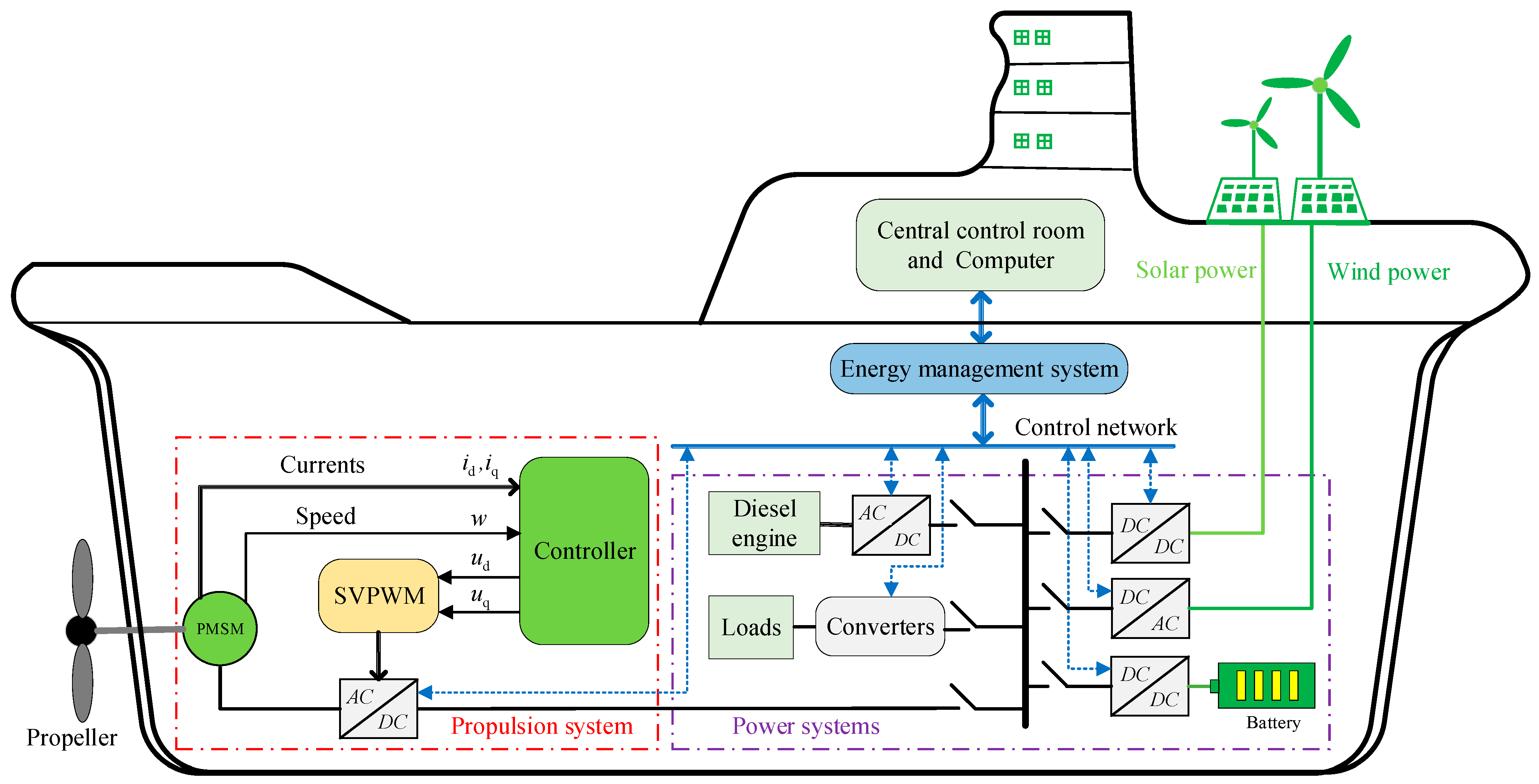The rest of this paper is structured as follows: Section 2 presents the structural framework of the new energy hybrid ship propulsion system and the construction of the PMSM mathematical model with matched or unmatched perturbations. Section 3 provides the design of the AFTCFBC to enable the output of the system to track the desired rotational speed within a finite period of time. Section 4 demonstrates the stability of the proposed AFTCFBC by applying Lyapunov theory. Section 5 outlines a simulation of the designed controller. Section 6 offers a summary and conclusions.

2. New Energy Hybrid Ship Propulsion System and Mathematical Modeling

In this section, an overview of the functions of each module in a novel energy hybrid ship is presented, and a mathematical model of the PMSM propulsion system is subsequently developed.

2.1. Hybrid Ship Propulsion System Architecture

In recent years, new energy hybrid ships have been developed with the objective of meeting the IMO’s carbon emission standards and of achieving comprehensive energy saving, energy storage, and efficient energy. Such ships employ diesel engines for the purpose of providing propulsion power and generating electricity, while solar photovoltaic panels and wind energy are utilized for auxiliary power generation and work together through inverters. This enables the optimization of the motor speed strategy in each sea state [36,37,38].

Figure 1 shows that in the new energy hybrid ship propulsion system, the entire system is monitored and controlled by the central control room and computer. The energy management system oversees the coordination of operational activities across all components via the control network. The primary source of energy for the vessel is the diesel engine, which transforms kinetic energy into electrical energy and then links to the power grid through an alternating-current/direct-current (AC/DC) inverter. The power from the grid can be supplied to various types of loads on the ship, either directly or via the inverters in the propulsion system. Solar energy and wind energy are converted into electricity by means of solar and wind power. This electricity can be utilized in two distinct ways. Initially, it can be transmitted via the transmission line, DC/DC inverter, and DC/AC inverter and subsequently connected directly to the power grid. This configuration serves as an auxiliary power unit for the ship’s power supply. Alternatively, the electricity can be transmitted through the DC/DC inverter and stored in the battery. This battery then releases the stored electricity when required.

In the propulsion system, the electric energy processed by the inverter is optimized and controlled by space vector pulse-width modulation (SVPWM), which then drives the PMSM to run. The PMSM outputs the rotational speed, which drives the propeller to rotate, thus enabling the propulsion of the ship. The system as a whole is capable of combining new and traditional energy sources through the collaborative work of all its parts. This allows it to utilize clean energy sources such as solar and wind in order to reduce carbon emissions, while also relying on the diesel engine to ensure the continuous operation of the ship and sufficient power to meet the needs of the new energy hybrid ship for long-distance voyages when necessary.

2.2. Mathematical Modeling of Ship Propulsion Motors

It is recommended that the mathematical model of a surface-mounted PMSM be represented in a synchronous rotating Cartesian coordinate system [39], as presented in Equation (1).

$$\left\{\begin{array}{l}J{\displaystyle \frac{dw}{dt}}=-Bw+{\displaystyle \frac{3}{2}}{P}_{\mathrm{n}}{\Psi }_{\mathrm{f}}{i}_{\mathrm{q}}-T_{\mathrm{L}}\\ L_{\mathrm{q}}{\displaystyle \frac{d{i}_{\mathrm{q}}}{dt}}=-P_{\mathrm{n}}{\Psi }_{\mathrm{f}}w-P_{\mathrm{n}}{L}_{\mathrm{q}}{i}_{\mathrm{d}}w-R_{\mathrm{s}}{i}_{\mathrm{q}}+u_{\mathrm{q}}\\ L_{\mathrm{d}}{\displaystyle \frac{d{i}_{\mathrm{d}}}{dt}}=P_{\mathrm{n}}{L}_{\mathrm{d}}{i}_{\mathrm{q}}w-R_{\mathrm{s}}{i}_{\mathrm{d}}+u_{\mathrm{d}}\end{array}\right.$$

(1)

where w represents the rotor mechanical angular velocity of the motor; P_n represents the pole pair number; Ψ_f represents the rotor flux linkage; J represents the rotational inertia; B represents the viscous damping friction coefficient; T_L is the load torque; R_s is the stator resistance; L_d and L_q represent the inductances of the stator on the d-q axis; i_d and i_q represent the currents of the stator on the d-q axis; and u_d and u_q represent the input voltages of the stator on the d-q axis.

In order to facilitate the design of the controller for the motor model in a more accurate and intuitive manner, a simplified motor model is illustrated in Equation (2).

$$\left\{\begin{array}{l}{\displaystyle \frac{dw}{dt}}=\Gamma w+{\lambda }_1{i}_{\mathrm{q}}+D\\ {\displaystyle \frac{d{i}_{\mathrm{q}}}{dt}}=P_{\mathrm{n}}\left({\lambda }_2-i_{\mathrm{d}}\right)w+{\mu }_1{i}_{\mathrm{q}}+{\displaystyle \frac{u_{\mathrm{q}}}{L_{\mathrm{s}}}}\\ {\displaystyle \frac{d{i}_{\mathrm{d}}}{dt}}=P_{\mathrm{n}}{i}_{\mathrm{q}}w+{\mu }_2{i}_{\mathrm{d}}+{\displaystyle \frac{u_{\mathrm{d}}}{L_{\mathrm{s}}}}\end{array}\right.$$

(2)

where ${\mu }_1,{\mu }_2$ are unknown parameters, the stator inductance $L_s=L_d=L_q,$ $\Gamma =-{\displaystyle \frac{B}{J}}, {\lambda }_1={\displaystyle \frac{1.5P_{\mathrm{n}}{\Psi }_{\mathrm{f}}}{J}}, {\lambda }_2=-{\displaystyle \frac{{\Psi }_{\mathrm{f}}}{L_{\mathrm{s}}}}, {\mu }_1=-{\displaystyle \frac{R_{\mathrm{s}}}{L_{\mathrm{q}}}}, {\lambda }_1={\displaystyle \frac{1.5P_{\mathrm{n}}{\Psi }_{\mathrm{f}}}{J}}, {\lambda }_2=-{\displaystyle \frac{{\Psi }_{\mathrm{f}}}{L_{\mathrm{s}}}}, {\mu }_1=-{\displaystyle \frac{R_{\mathrm{s}}}{L_{\mathrm{q}}}}.$ As stated in [36], system (2) is a nonlinear equation in semi-strict feedback form, in which w, i_d and i_q are regarded as the state variables of the system.

The subsequent three lemmas are introduced: The first and second lemmas are employed to prove the stability of the AFTCFBC and to analyze it in this paper. The third is used to prove the stability of the NFTCF and to analyze it [40].

Lemma 1.

For any positive constants c and d and any real function $\eta (x,y)>0$, the following inequality holds: ${\left|x\right|}^{\mathrm{c}}{\left|y\right|}^{\mathrm{d}}\le {\displaystyle \frac{c}{c+d}}\eta (x,y){\left|x\right|}^{\mathrm{c}+\mathrm{d}}+{\displaystyle \frac{d}{c+d}}{\eta }^{-\mathrm{c}/\mathrm{d}}(x,y){\left|y\right|}^{\mathrm{c}+\mathrm{d}}$.

Lemma 2.

Consider a nonlinear system where there is a function $V\left(x\right)>0$ on ${ℂ}^1$ and $\dot{V}\left(x\right)\le -k{V}^{\alpha }\left(x\right)+ϵ, k>0, ϵ>0, 0<\alpha <1$, which is pragmatically stable in finite time.

Lemma 3.

Consider a nonlinear system where there is a function $V\left(x\right)>0$ on ${ℂ}^1$ and $\dot{V}\left(x\right)\le -k{V}^{\alpha }\left(x\right)-bV\left(x\right), k>0, 0<\alpha <1$, which is fast and stable in finite time.

3. AFTCFBC Design

This section of the paper is concerned with the issue of how to achieve effective improvement in the control of the ship’s PMSM parameters in the context of unknown load disturbance variations in a complex marine environment. In doing so, it considers the phenomenon of controller oscillation and overshoot, which may occur as a result of jitter vibration during the SMC process. 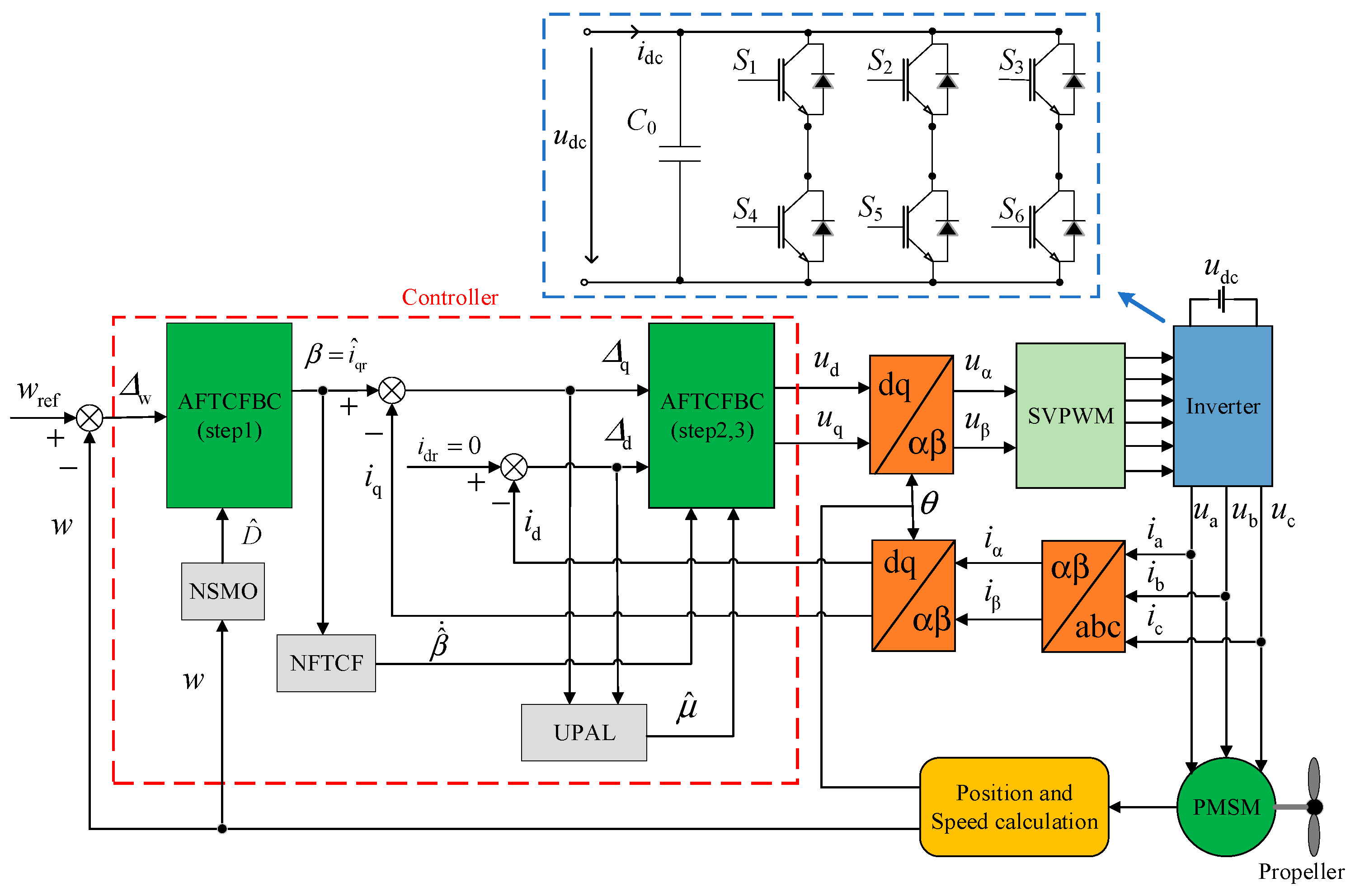In order to achieve the accurate tracking of the nonlinear system (2) output (w) relative to the reference signal (w_ref) within a finite time frame, an AFTCFBC control strategy is proposed. 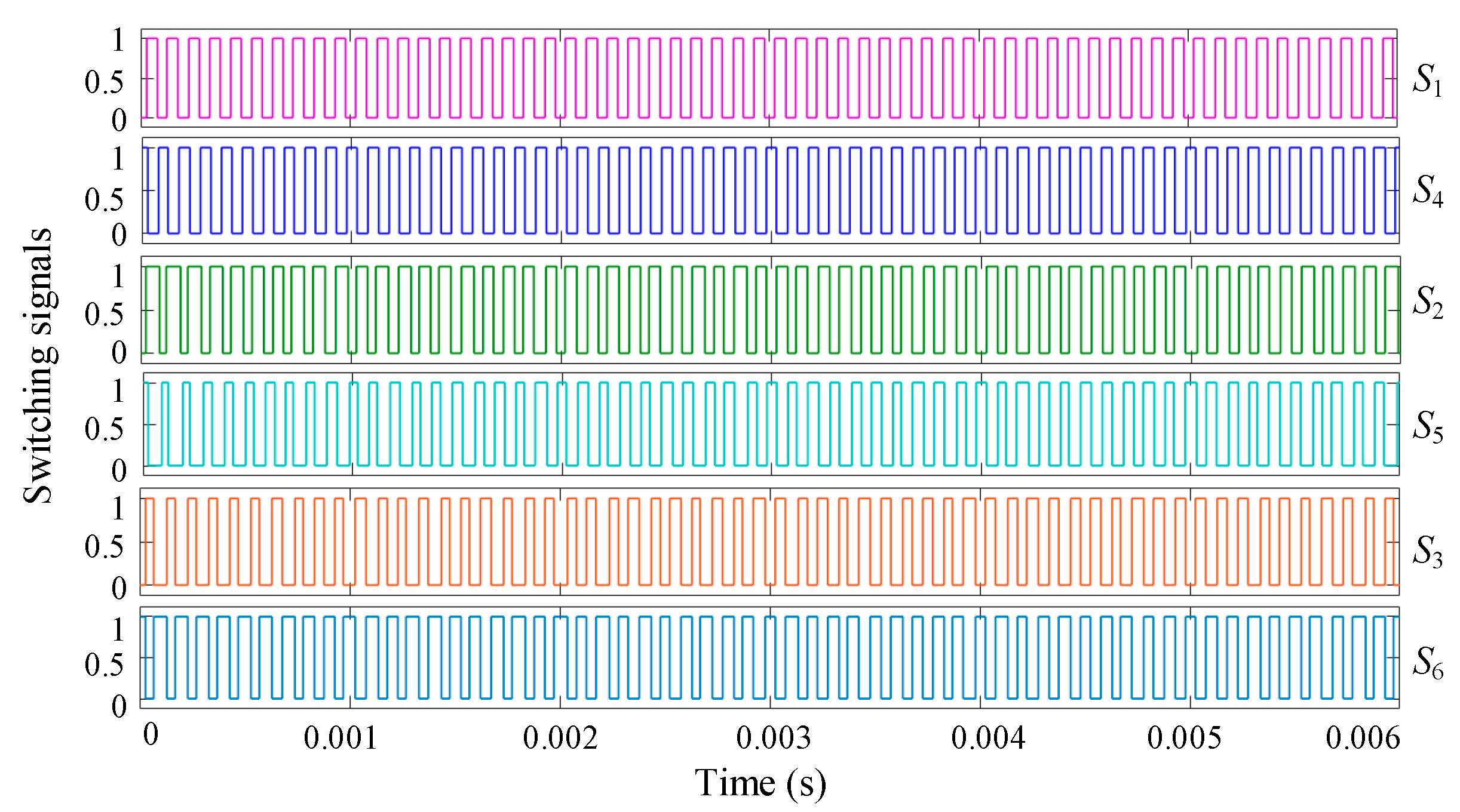The block diagram of the controller structure is divided into two sections: outer-loop speed control and single inner-loop current control, as expressed in Figure 2. The configuration of the inverter depicted in the figure comprises C₀, which denotes capacitance, u_dc, representing the inverter’s DC-side voltage, and i_dc for the inverter’s DC-side current. Additionally, S₁, S₂, S₃, S₄, S₅, and S₆ refer to six switching signals, with the input being facilitated by SVPWM. In this configuration, the transistors of SVPWM act as switching devices.

Step 1 involves the construction of the virtual current controller via NSMC. Steps 2 and 3 then proceed with the design of the d-axis and q-axis voltage controllers, utilizing the virtual control currents i_qr, NFTCF, and UPAL to obtain the control signals (u_d, u_q). The control signals u_d and u_q are transformed in a series of steps, beginning with an inverse Park transform, followed by space vector pulse-width modulation (SVPWM), an inverter, and finally a Clarke transform. This sequence of transformations is used to obtain the direct (i_d) and intersection (i_q) currents, which are then fed back to the controller as part of a single inner-loop current feedback control loop. In the field of motor control, the Park and Clarke transforms are two widely used mathematical transformations that facilitate the conversion of variables in a three-phase (abc) coordinate system into a two-phase (αβ) stationary coordinate system, as well as the synchronous rotation of direct-axis (d) and cross-axis (q) coordinate systems. This enables the development of more intuitive and efficient control strategies. The inverter is responsible for converting the direct-current power supply to an alternating-current power supply. The SVPWM technique is a common inverter control technique that precisely controls the output voltage waveform and frequency by adjusting the pulse width. The rotor position (θ) and speed (w) of the PMSM are obtained from the position and speed calculation module, which constitutes the external-loop speed feedback control of the controller. This results in a cascaded dual closed-loop vector control strategy.

3.1. Designing Nonlinear Finite-Time Command Filter

The designed command filter can be employed to address the issue of the complexity of the differential derivative calculation resulting from the implementation of backstepping control, thereby reducing the maximum steady-state error of the system output as expressed in Equation (3).

$$\dot{\widehat{\beta }}=\left[\zeta \left(w,t\right)+{\displaystyle \frac{\xi \left(t\right)}{{\left|\tilde{\beta }\right|}^{\mathrm{r}}+\rho }}\right]\tilde{\beta }+\delta \tilde{\beta }$$

(3)

where $\tilde{\beta }=\beta -\widehat{\beta }, \beta ={\widehat{i}}_{\mathrm{qr}}, {\widehat{i}}_{\mathrm{qr}}$ denotes the cross-axis desired virtual current control quantity, as shown in Figure 2. $\widehat{\beta }$ is the estimated state signal β, and β denotes the virtual current filtering signal, the design procedure for which is outlined in Section 3.2.2. Additionally, 0 < r < 1, r, δ is a positive constant. In this particular study, we have set r = 0.5.

In Equation (3), $\zeta \left(w,t\right)$ and $\xi \left(t\right)$ denote monotonically bounded functions with respect to the variable t, with the stipulation that both functions must be non-negative. The design of $\zeta \left(w,t\right)$ for distinct rotational speeds, denoted by $w$, enables the dynamic adjustment of the filter’s (3) filtering capability in response to the variation in rotational speed, $w$. Assume that the state signal β and its first-order derivatives are bounded. In this case, the filter error $\tilde{\beta }$ will converge to a value close to zero within a finite time frame.

The present study analyzes the stability of command filters in the context of Lyapunov candidate functions, as expressed in Equation (4).

$$V_{\beta }={\displaystyle \frac{1}{2}}{\tilde{\beta }}^2$$

(4)

The derivation of $V_{\beta }$ ultimately yields Inequation (5).

$$\begin{array}{cc}\hfill {\dot{V}}_{\beta }& =\tilde{\beta }\left(\dot{\beta }-\dot{\widehat{\beta }}\right)\hfill \\ & =\tilde{\beta }\left[\dot{\beta }-\zeta \left(w,t\right)\tilde{\beta }-{\displaystyle \frac{\xi \left(t\right)\tilde{\beta }}{{\left|\tilde{\beta }\right|}^{1/2}+\rho }}-\tilde{\beta }\delta \right]\\ & \le -\left(\zeta \left(w,t\right)+\delta \right){\tilde{\beta }}^2-{\displaystyle \frac{\xi \left(t\right){\tilde{\beta }}^2}{{\left|\tilde{\beta }\right|}^{1/2}+\rho }}+\tilde{\beta }\dot{\beta }\\ & \le -\left(\zeta \left(w,t\right)+\delta \right){\tilde{\beta }}^2-{\left|\tilde{\beta }\right|}^{1/2}\left[{\displaystyle \frac{\xi \left(t\right){\left|\tilde{\beta }\right|}^{3/2}}{{\left|\tilde{\beta }\right|}^{1/2}+\rho }}-{\left|\tilde{\beta }\right|}^{1/2}\dot{\beta }\right]\end{array}$$

(5)

If there exists a positive constant M such that $\xi {\left(t\right)}_{\min }=M>{\left|\dot{\beta }\right|}_{\max }=\sigma >0$ and there exists $M=h\sigma , h>0$, then there exists the inequality shown in Inequation (6).

$$\begin{array}{cc}\hfill {\dot{V}}_{\beta }& \le -L{\tilde{\beta }}^2-{\left|\tilde{\beta }\right|}^{1/2}\left[{\displaystyle \frac{h\sigma {\left|\tilde{\beta }\right|}^{3/2}}{{\left|\tilde{\beta }\right|}^{1/2}+\rho }}-{\left|\tilde{\beta }\right|}^{1/2}\sigma \right]\hfill \\ & \le -L{\tilde{\beta }}^2-\sigma {\left|\tilde{\beta }\right|}^{3/2}\left[{\displaystyle \frac{h{\left|\tilde{\beta }\right|}^{1/2}}{{\left|\tilde{\beta }\right|}^{1/2}+\rho }}-{\displaystyle \frac{1}{{\left|\tilde{\beta }\right|}^{1/2}}}\right]\hfill \end{array}$$

(6)

where $L=\zeta \left(w,t\right)+\delta$.

When satisfying $\rho \ge {\displaystyle \frac{\left(2h-1\right)\left|\tilde{\beta }\right|-{\left|\tilde{\beta }\right|}^{1/2}}{{\left|\tilde{\beta }\right|}^{1/2}+1}}, \rho >0$, we have ${\displaystyle \frac{h{\left|\tilde{\beta }\right|}^{3/2}}{{\left|\tilde{\beta }\right|}^{1/2}+\rho }}-{\displaystyle \frac{1}{{\left|\tilde{\beta }\right|}^{1/2}}}\le 1$, and if there exists a positive constant m such that at this point $\zeta {\left(w,t\right)}_{\min }=m_0$, then we can obtain the equation shown in Equation (7).

$$\begin{array}{cc}\hfill {\dot{V}}_{\beta }& \le -L{\tilde{\beta }}^2-\sigma {\left|\tilde{\beta }\right|}^{3/2}\hfill \\ & \le -2m{V}_{\beta }-{\displaystyle \frac{\sigma }{2}}{V_{\beta }}^{3/4}\hfill \end{array}$$

(7)

where $m=m_0+\delta$.

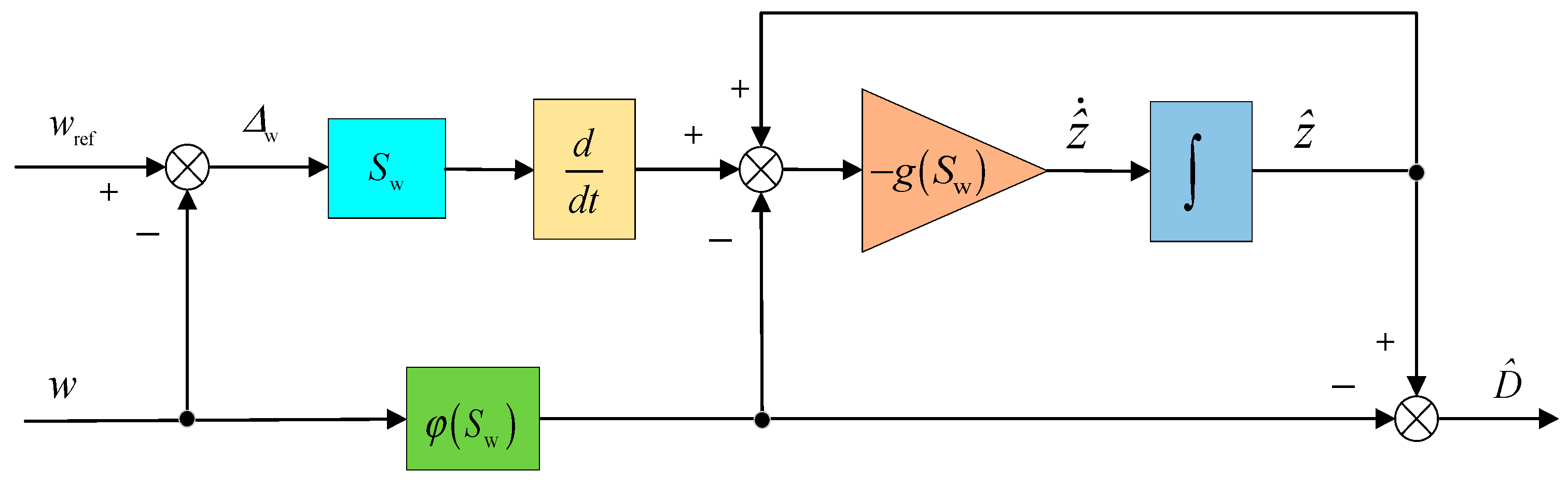
According to Lemma 3, the nonlinear command filter (3) is finite-time-stable. The control structure diagram of the filter shown in Figure 3 is constructed, and the stability of the proposed NFTCF is verified by simulation.

The input signal β(t) is given by Equation (8).

$$\begin{array}{cc}\beta \left(t\right)=\left\{\begin{array}{l}60,\\ 60+20\sin \left(f^{\ast }2\pi t\right),\\ 40+10t, \end{array}\right.& \begin{array}{l}0\le t<0.5, \hfill \\ 0.5\le t<2, \hfill \\ 2\le t<3.\hfill \end{array}\end{array}$$

(8)

where f is the signal frequency in Hertz (Hz).

The nonlinear function is shown in Equation (9).

$$\left\{\begin{array}{l}\zeta \left(w,t\right)=l_1{e}^{-{\displaystyle \frac{l_2}{w\left(t\right)+20}}}\\ \xi \left(t\right)=l_3\tanh \left(l_{4}t\right)\end{array}\right.$$

(9)

where $l_1, l_2, l_3, l_4$ are positive constants, the specific values of which are related to β and w(t); in this paper, $l_1=90, l_2=200, l_3=200, l_4=6$. The given signal w(t) is a random white noise interference signal superimposed at the speed of 500 r/min.

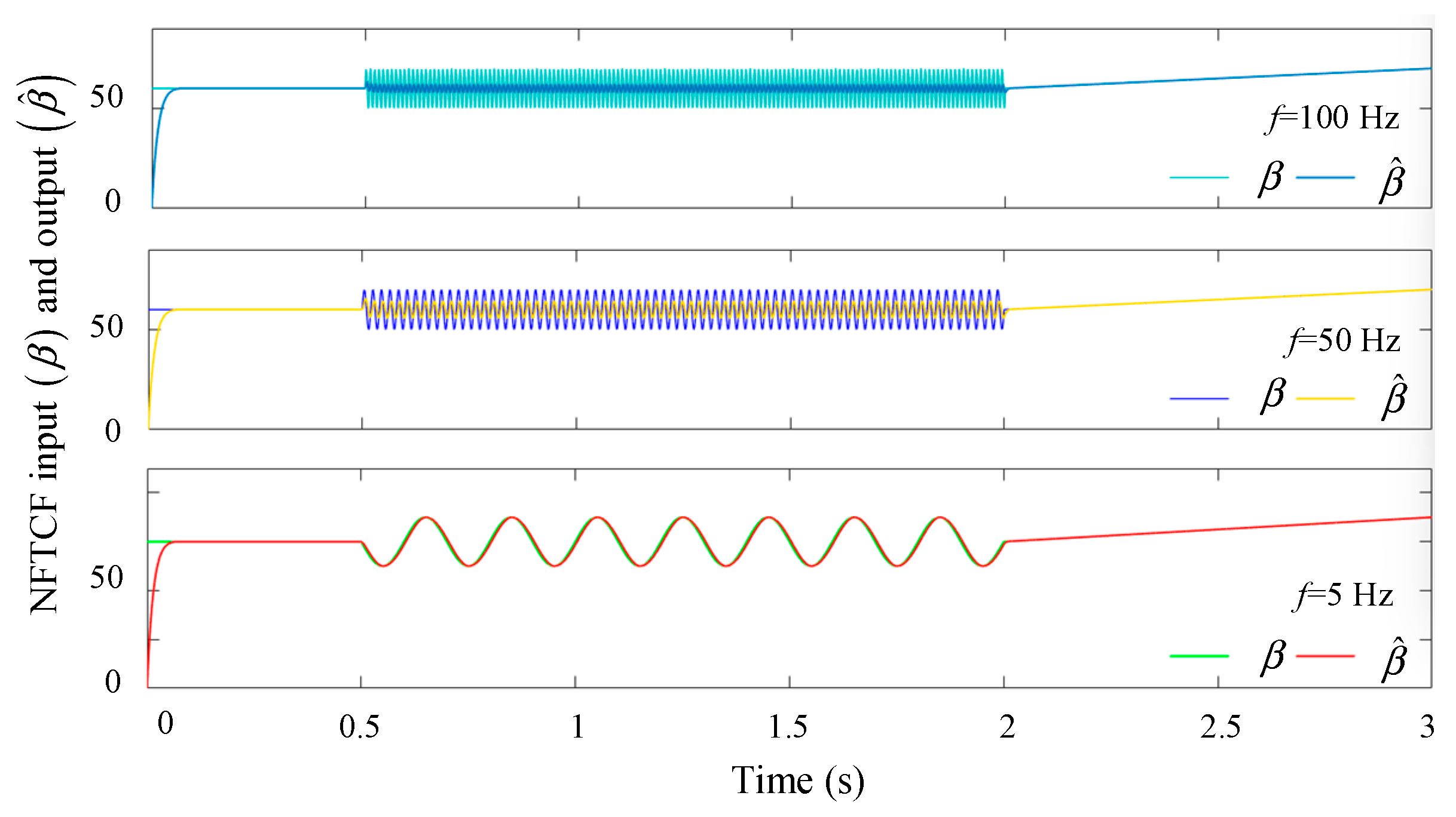
The tracking performance of the NFTCF output $\widehat{\beta }$ signal, which is tracked at different frequencies (f = 5 Hz, 50 Hz, 100 Hz) of the input β signal, is analyzed through simulations. The effect of the input signal β at different frequencies on the stability of the filter is investigated through these simulations. The parameters $\rho , \sigma$ of Equation (3) are analyzed for their effect on the filter’s stability under the selected input signal β of the same frequency. The values of their best performance are selected. The results of these analyses can be found in Figure 4, Figure 5, Figure 6 and Figure 7.

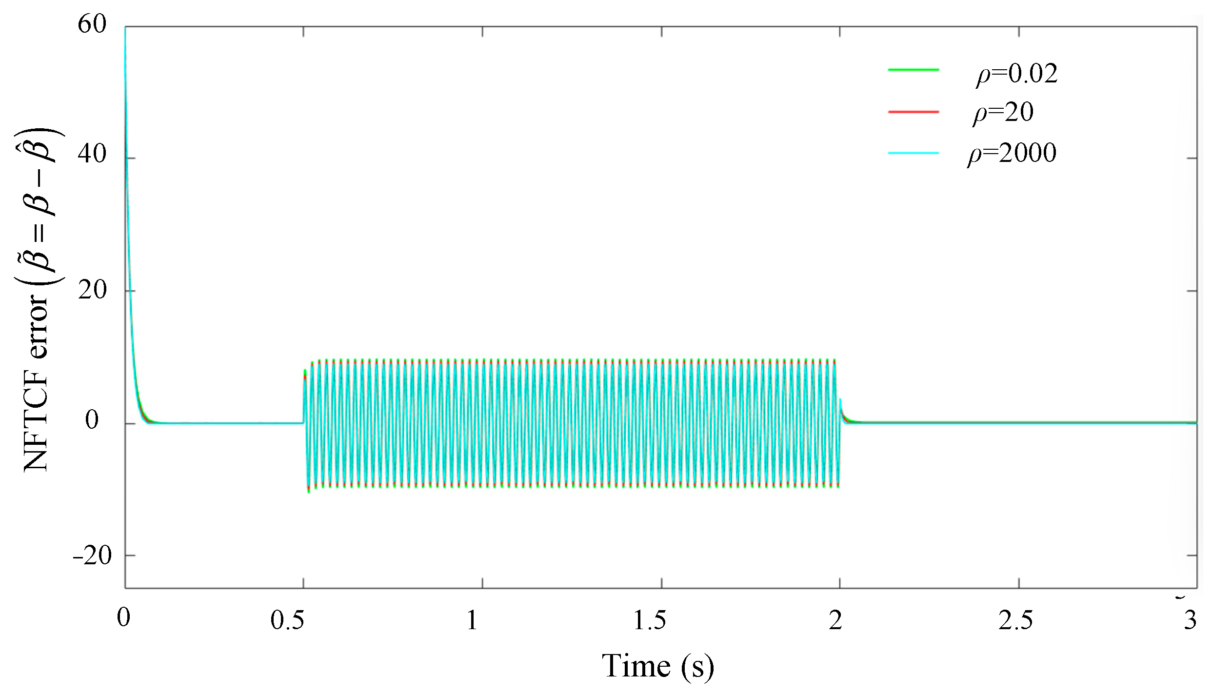
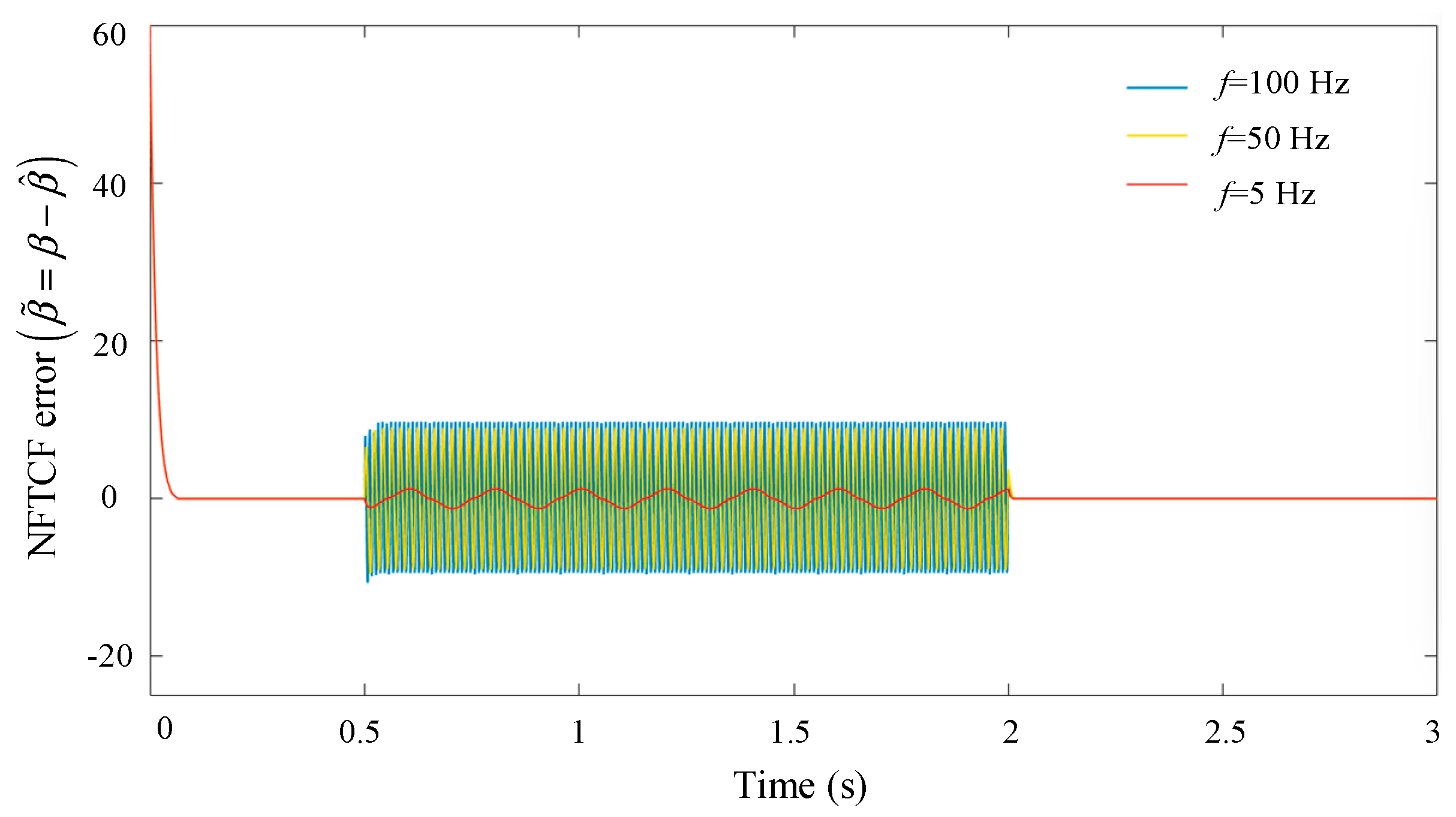
As demonstrated in Figure 4, Figure 5, Figure 6 and Figure 7, the designed filter demonstrates superior tracking performance in the low-frequency band. Conversely, the tracking error $\tilde{\beta }$ increases with the frequency of the input signal β and decreases with the parameters ρ and δ. Concurrently, the response speed accelerates.

As demonstrated in Figure 3 and Figure 4 and in accordance with Equation (3), the filter exhibits low-pass characteristics, thereby attenuating high-frequency signals more significantly than low-frequency signals. Consequently, in scenarios where the input signal comprises a substantial proportion of high-frequency components, the signal undergoes significant attenuation upon filtration, resulting in increased signal distortion and error.

3.2. Designing Backstepping Sliding Mode Controller

In accordance with the tenets of backstepping sliding mode control theory, the exponentially decaying sliding mode surface is given by the equation $S=\Delta -\Delta \left(0\right)e^{-\gamma \mathrm{t}}$, wherein $\angle$ represents the state error, $\Delta \left(0\right)$ denotes the initial value, and γ is a positive constant. Given that system (2) is an equation in semi-strict feedback form, the objective of employing backstepping control is to effectively eliminate the state variable errors in the rotational speed (w) and current ($i_{\mathrm{q}}, i_{\mathrm{d}}$) in system (2) through the feedback mechanism and to achieve high-precision control of the output.

3.2.1. Design of d-q-Axis Voltage Input Controller

In consideration of the second and third equations in the PMSM system (2), the design of the q-axis current sliding mode function is presented in Equation (10).

$$S_{\mathrm{q}}={\Delta }_{\mathrm{q}}-{\Delta }_{\mathrm{q}}\left(0\right)e^{-{\gamma }_{\mathrm{q}}\mathrm{t}}$$

(10)

where ${\gamma }_{\mathrm{q}}$ is a positive constant, speed error ${\Delta }_{\mathrm{q}}={\widehat{i}}_{\mathrm{qr}}-i_{\mathrm{q}}, {\widehat{i}}_{\mathrm{qr}}=\beta$ denotes the cross-axis desired virtual current state variable, and ${\Delta }_{\mathrm{q}}\left(0\right)={\widehat{i}}_{\mathrm{qr}}\left(0\right)-i_q\left(0\right)$, wherein ${\widehat{i}}_{\mathrm{qr}}\left(0\right)$ and $i_{\mathrm{q}}\left(0\right)$ represent the initial value.

The differential equation of the closed-loop tracking error is derived from the sliding mode function $S_{\mathrm{q}}$ and analyzed using Lyapunov stability theory as outlined below.

It is imperative to consider the Lyapunov candidate function $V_1=V_{\beta }+V_{\mathrm{q}}$ in Equation (11), wherein $V_{\mathrm{q}}={\displaystyle \frac{1}{2}}{S}_{\mathrm{q}}^2$.

$$V_1=V_{\beta }+{\displaystyle \frac{1}{2}}{S}_{\mathrm{q}}^2$$

(11)

The derivation of $V_1$ is shown in Equation (12).

$${\dot{V}}_1={\dot{V}}_{\beta }+S_{\mathrm{q}}\left[{\dot{\widehat{i}}}_{\mathrm{qr}}-P_{\mathrm{n}}\left({\lambda }_2-i_{\mathrm{d}}\right)w-{\mu }_1{i}_{\mathrm{q}}-{\displaystyle \frac{u_{\mathrm{q}}}{L_{\mathrm{s}}}}+\right.\left.{\gamma }_{\mathrm{q}}{\Delta }_{\mathrm{q}}\left(0\right)e^{-{\gamma }_{\mathrm{q}}\mathrm{t}}\right]$$

(12)

where ${\dot{\widehat{i}}}_{\mathrm{qr}}$ is the q-axis desired virtual current state derivative, and ${\dot{\widehat{i}}}_{\mathrm{qr}}=\dot{\widehat{\beta }}$.

Subsequently, the q-axis voltage input controller is designed as shown in Equation (13).

$$u_{\mathrm{q}}=L_{\mathrm{s}}\left[K_{\mathrm{q}}{S}_{\mathrm{q}}+\dot{\widehat{\beta }}-P_{\mathrm{n}}\left({\lambda }_2-i_{\mathrm{d}}\right)w-\right.\left.{\widehat{\mu }}_1{i}_{\mathrm{q}}+{\gamma }_{\mathrm{q}}{\Delta }_{\mathrm{q}}\left(0\right)e^{-{\gamma }_{\mathrm{q}}\mathrm{t}}\right]$$

(13)

where $K_{\mathrm{q}}$ is a positive constant and ${\widehat{\mu }}_1$ represents an estimate of the parameter ${\mu }_1$, and its design process is given in Section 3.3.2.

In the absence of consideration of the parameter-adaptive law design (${\widehat{\mu }}_1={\mu }_1$) and taking $u_{\mathrm{q}}$ into account in Equation (12), we obtain in Equation (14).

$$\begin{array}{cc}\hfill {\dot{V}}_1& =\tilde{\beta }\left(\dot{\beta }-\dot{\widehat{\beta }}\right)-K_{\mathrm{q}}{S}_{\mathrm{q}}^2\hfill \\ & \le -K_{\mathrm{q}}{S}_{\mathrm{q}}^2-2m{V}_{\beta }-{\displaystyle \frac{\sigma }{2}}{V_{\beta }}^{3/4}\hfill \\ & \le -2K_{\mathrm{q}}{V}_{\mathrm{q}}-2m{V}_{\beta }+C_1\hfill \\ & \le -2{\varphi }_1{V}_1+C_1\hfill \end{array}$$

(14)

where ${\varphi }_1=\min \left\{K_{\mathrm{q}}, m\right\}, C_1\ge 0$.

Upon analysis of the aforementioned integral inequality (14), it becomes evident that if ${\varphi }_1>C_1/2{\tau }_1\left({\tau }_1>0\right)$, when $V_1={\tau }_1, {\dot{V}}_1\le -2{\varphi }_1{\tau }_1+C_1$, there is ${\dot{V}}_1\le 0$. This signifies that ${\dot{V}}_1\le {\tau }_1$ is an invariant set $V_1\left(t\right)\le {\tau }_1\left(t\ge 0\right)$ with respect to $V_1={\tau }_1$, as illustrated in Equation (15).

$$0\le V_1\left(t\right)\le {\varphi }_1+\left(V_1\left(0\right)-{\varphi }_1\right)e^{-2{\varphi }_{1}t}, \forall t\ge 0$$

(15)

The analysis of Equation (15) shows that $V_1\left(t\right)$ is subject to the constraint ${\varphi }_1$. This observation leads to the conclusion that $S_{\mathrm{q}}$ is bounded. Therefore, when the sliding mode exponential function $S_{\mathrm{q}}={\Delta }_{\mathrm{q}}-{\Delta }_{\mathrm{q}}\left(0\right)e^{{-\gamma }_{\mathrm{q}}\mathrm{t}}$ is utilized as a Lyapunov function, it can be ensured that the system is globally exponentially stable and the q-axis current error ${\Delta }_{\mathrm{q}}$ will converge to zero in finite time.

Similarly, the d-axis current sliding mode function is designed in Equation (16).

$$S_{\mathrm{d}}={\Delta }_{\mathrm{d}}-{\Delta }_{\mathrm{d}}\left(0\right)e^{-{\gamma }_{\mathrm{d}}\mathrm{t}}$$

(16)

where ${\gamma }_{\mathrm{d}}$ is a positive constant and speed error ${\Delta }_{\mathrm{d}}={\widehat{i}}_{\mathrm{dr}}-i_{\mathrm{d}}, {\Delta }_{\mathrm{d}}\left(0\right)={\widehat{i}}_{\mathrm{dr}}\left(0\right)-i_{\mathrm{d}}\left(0\right)$, wherein ${\widehat{i}}_{\mathrm{dr}}\left(0\right)$ and $i_{\mathrm{d}}\left(0\right)$ represent the initial value. Assume that ${\widehat{i}}_{\mathrm{dr}}=0$.

The differential equation of the closed-loop tracking error is derived from the sliding mode function $S_{\mathrm{d}}$ and analyzed using Lyapunov stability theory as outlined below.

It is imperative to consider the Lyapunov candidate function $V_2=V_1+V_{\mathrm{d}}$ in Equation (17), wherein $V_{\mathrm{d}}={\displaystyle \frac{1}{2}}{S}_{\mathrm{d}}^2$.

$$V_2=V_1+{\displaystyle \frac{1}{2}}{S}_{\mathrm{d}}^2$$

(17)

The derivation of $V_2$ is shown in Equation (18).

$${\dot{V}}_2={\dot{V}}_1+S_{\mathrm{d}}\left[{\dot{\widehat{i}}}_{\mathrm{dr}}-P_{\mathrm{n}}{i}_{\mathrm{q}}w-{\mu }_2{i}_{\mathrm{d}}-{\displaystyle \frac{u_{\mathrm{d}}}{L_{\mathrm{s}}}}+\right.\left.{\gamma }_{\mathrm{d}}{\Delta }_{\mathrm{d}}\left(0\right){\mathrm{e}}^{-{\gamma }_{\mathrm{d}}\mathrm{t}}\right]$$

(18)

where ${\dot{\widehat{i}}}_{\mathrm{dr}}$ is the d-axis desired virtual current state derivative, and ${\dot{\widehat{i}}}_{\mathrm{dr}}=0$.

Subsequently, the d-axis voltage input controller is designed as shown in Equation (19).

$$u_{\mathrm{d}}=L_{\mathrm{s}}\left[K_{\mathrm{d}}{S}_{\mathrm{d}}-P_{\mathrm{n}}{i}_{\mathrm{q}}w-{\widehat{\mu }}_2{i}_{\mathrm{d}}+\right.\left.{\gamma }_{\mathrm{d}}{\Delta }_{\mathrm{d}}\left(0\right)e^{-{\gamma }_{\mathrm{d}}\mathrm{t}}\right]$$

(19)

where $K_{\mathrm{d}}$ is a positive constant and ${\widehat{\mu }}_2$ represents an estimate of the parameter ${\mu }_2$, and its design process is given in Section 3.3.2.

In the absence of consideration of the parameter-adaptive law design (${\widehat{\mu }}_1={\mu }_1, {\widehat{\mu }}_2={\mu }_2$) and taking $u_{\mathrm{d}}$ into account in Equation (18), we obtain in Equation (20).

$$\begin{array}{cc}\hfill {\dot{V}}_2& ={\dot{V}}_1-K_{\mathrm{d}}{S}_{\mathrm{d}}^2\hfill \\ & \le -2K_{\mathrm{q}}{V}_{\mathrm{q}}-2K_{\mathrm{d}}{V}_{\mathrm{d}}-2m{V}_{\beta }+C_2\hfill \\ & \le -2{\varphi }_2{V}_2+C_2\hfill \end{array}$$

(20)

where ${\varphi }_2=\min \left\{K_{\mathrm{q}}, K_{\mathrm{d}}, m\right\}, C_2\ge 0$.

It is evident that an identical analytical process to that delineated in Equation (14) results in the derivation of in Equation (21).

$$0\le V_2\left(t\right)\le {\varphi }_2+\left(V_2\left(0\right)-{\varphi }_2\right)e^{-2{\varphi }_{2}t}, \forall t\ge 0$$

(21)

The analysis of Equation (21) shows that $V_2\left(t\right)$ is subject to the constraint ${\varphi }_2$. This observation leads to the conclusion that $S_{\mathrm{q}}, S_{\mathrm{d}}$ are bounded. Therefore, when the sliding mode exponential function $S_{\mathrm{d}}={\Delta }_{\mathrm{d}}-{\Delta }_{\mathrm{d}}\left(0\right)e^{-{\gamma }_{\mathrm{d}}\mathrm{t}}$ is utilized as a Lyapunov function, it can be ensured that the system is globally exponentially stable and the d-axis current error ${\Delta }_{\mathrm{d}}$ will converge to zero in finite time.

3.2.2. Designing a Virtual Current Filter Controller

Given the first equation of the PMSM system (2), the function $S_{\mathrm{w}}$ of the speed sliding mode is designed as expressed in Equation (22).

$$S_{\mathrm{w}}={\Delta }_{\mathrm{w}}-{\Delta }_{\mathrm{w}}\left(0\right)e^{{-\gamma }_{\mathrm{w}}\mathrm{t}}$$

(22)

where ${\gamma }_{\mathrm{w}}$ is a positive constant, speed error ${\Delta }_{\mathrm{w}}=w_{\mathrm{ref}}-w$, wherein $w_{\mathrm{ref}}$ denotes the given desired reference speed input. ${\Delta }_{\mathrm{w}}\left(0\right)=w_{\mathrm{ref}}\left(0\right)-w\left(0\right)$, wherein $w_{\mathrm{ref}}\left(0\right)$ and $w\left(0\right)$ denotes the initial value.

The differential equation of the closed-loop tracking error is derived from the sliding mode function $S_{\mathrm{w}}$ and analyzed using Lyapunov stability theory as outlined below.

It is imperative to consider the Lyapunov candidate function $V_3=V_2+V_{\mathrm{w}}$ in Equation (23), wherein $V_{\mathrm{w}}={\displaystyle \frac{1}{2}}{S}_{\mathrm{w}}^2$.

$$V_3=V_2+{\displaystyle \frac{1}{2}}{S}_{\mathrm{w}}^2$$

(23)

The derivation of $V_3$ is shown in Equation (24).

$${\dot{V}}_3={\dot{V}}_2+S_{\mathrm{w}}\left[{\dot{w}}_{\mathrm{ref}}-\Gamma w+{\lambda }_1{\Delta }_{\mathrm{q}}-{\lambda }_1\tilde{\beta }-{\lambda }_1\beta -D\right.+\left.{\gamma }_{\mathrm{w}}{\Delta }_{\mathrm{w}}\left(0\right)e^{-{\gamma }_{\mathrm{w}}\mathrm{t}}\right]$$

(24)

where the cross-axis current error ${\Delta }_{\mathrm{q}}={\widehat{i}}_{\mathrm{qr}}-i_{\mathrm{q}}$, wherein cross-axis current virtual control ${\widehat{i}}_{\mathrm{qr}}$ is designed as ${\widehat{i}}_{\mathrm{qr}}=\beta$.

Subsequently, the virtual current filtering control $\beta$ signal is designed as shown in Equation (25).

$$\beta ={\displaystyle \frac{1}{{\lambda }_1}}\left[K_{\mathrm{w}}{S}_{\mathrm{w}}+{\dot{w}}_{\mathrm{ref}}-\Gamma w-\widehat{D}+\right.\left.{\gamma }_{\mathrm{w}}{\Delta }_{\mathrm{w}}\left(0\right)e^{-{\gamma }_{\mathrm{w}}\mathrm{t}}\right]$$

(25)

where $\widehat{D}$ is an estimate of D, and its design process is given in Section 3.3.1.

In the absence of consideration of the parameter-adaptive law design (${\widehat{\mu }}_1={\mu }_1, {\widehat{\mu }}_2={\mu }_2$) and the disturbance estimation design ($\widehat{D}=D$) and taking $\beta$ into account in Equation (24), we obtain in Equation (26).

$$\begin{array}{cc}\hfill {\dot{V}}_3& ={\dot{V}}_2+S_{\mathrm{w}}\left(-K_{\mathrm{w}}{S}_{\mathrm{w}}+{\lambda }_1{\Delta }_{\mathrm{q}}-{\lambda }_1\tilde{\beta }\right)\hfill \\ & =-K_{\mathrm{w}}{S}_{\mathrm{w}}^2-K_{\mathrm{q}}{S}_{\mathrm{q}}^2-K_{\mathrm{d}}{S}_{\mathrm{d}}^2+{\lambda }_1{\Delta }_{\mathrm{q}}{S}_{\mathrm{w}}-{\lambda }_1\tilde{\beta }{S}_{\mathrm{w}}+{\dot{V}}_{\beta }\hfill \\ & \le \left({\displaystyle \frac{3{\lambda }_1}{2}}-K_{\mathrm{w}}\right)S_{\mathrm{w}}^2+\left({\displaystyle \frac{{\lambda }_1}{2}}-K_{\mathrm{q}}\right)S_{\mathrm{q}}^2-K_{\mathrm{d}}{S}_{\mathrm{d}}^2+{\displaystyle \frac{{\lambda }_1}{2}}{\tilde{\beta }}^2-2m{V}_{\beta }-{\displaystyle \frac{\sigma }{2}}{V}_{\beta }^{3/4}+{\displaystyle \frac{{\lambda }_1}{2}}{\Delta }_{\mathrm{q}}^2\left(0\right)e^{-2{\gamma }_{\mathrm{q}}\mathrm{t}}\hfill \\ & \le -2\left(K_{\mathrm{w}}-{\displaystyle \frac{3{\lambda }_1}{2}}\right)V_{\mathrm{w}}-2\left(K_{\mathrm{q}}-{\displaystyle \frac{{\lambda }_1}{2}}\right)V_{\mathrm{q}}-2K_{\mathrm{d}}{V}_{\mathrm{d}}-2\left(m-{\displaystyle \frac{{\lambda }_1}{2}}\right)V_{\beta }+{\displaystyle \frac{{\lambda }_1}{2}}{\Delta }_{\mathrm{q}}^2\left(0\right)e^{-2{\gamma }_{\mathrm{q}}\mathrm{t}}\hfill \\ & \le -2{\varphi }_3{V}_3+C_3\hfill \end{array}$$

(26)

where ${\varphi }_3=\min \left\{K_{\mathrm{w}}-{\displaystyle \frac{3{\lambda }_1}{2}}, K_{\mathrm{q}}-{\displaystyle \frac{{\lambda }_1}{2}}, K_{\mathrm{d}}, m-{\displaystyle \frac{{\lambda }_1}{2}}\right\}, C_3={\displaystyle \frac{{\lambda }_1}{2}}{\Delta }_{\mathrm{q}}^2\left(0\right)e^{-2{\gamma }_{\mathrm{q}}\mathrm{t}}$.

It is evident that an identical analytical process to that delineated in Equation (14) results in the derivation of in Equation (27).

$$0\le V_3\left(t\right)\le {\varphi }_3+\left(V_3\left(0\right)-{\varphi }_3\right)e^{-2{\varphi }_{3}t}, \forall t\ge 0$$

(27)

The analysis of Equation (27) shows that $V_3\left(t\right)$ is subject to the constraint ${\varphi }_3$. This observation leads to the conclusion that $S_{\mathrm{w}}, S_{\mathrm{q}}, S_{\mathrm{d}}$ are all bounded. Therefore, when the sliding mode exponential function $S_{\mathrm{w}}={\Delta }_{\mathrm{w}}-{\Delta }_{\mathrm{w}}\left(0\right)e^{-{\gamma }_{\mathrm{w}}\mathrm{t}}$ is utilized as a Lyapunov function, it can be ensured that the system is globally exponentially stable and the speed error ${\Delta }_{\mathrm{w}}$ will converge to zero in finite time.

3.3. Designing NSMO and UPAL

3.3.1. Designing Exponential Nonlinear Sliding Mode Observer

A nonlinear function is introduced for the NSMO to estimate the load torque, and the design is shown in Equation (28).

$$\left\{\begin{array}{l}\widehat{D}=\widehat{z}-\phi \left(S_{\mathrm{w}}\right)\hfill \\ \dot{\widehat{z}}=-g\left(S_{\mathrm{w}}\right)\left[\Phi +\widehat{z}+\phi \left(S_{\mathrm{w}}\right)\right]\hfill \end{array}\right.$$

(28)

where $\Phi ={\dot{w}}_{\mathrm{ref}}-\Gamma w-{\lambda }_1{i}_{\mathrm{q}}+{\gamma }_{\mathrm{w}}{\Delta }_{\mathrm{w}}\left(0\right){\mathrm{e}}^{-{\gamma }_{\mathrm{w}}\mathrm{t}}, \phi \left(S_{\mathrm{w}}\right)$ is actually designed according to the need for a nonlinear function, and $g\left(S_{\mathrm{w}}\right)={\displaystyle \frac{\partial \phi \left(S_{\mathrm{w}}\right)}{\partial S_{\mathrm{w}}}}$ is a bounded function, wherein $g\left(S_{\mathrm{w}}\right)$ is designed to resist the perturbation caused by changes in the external environment, and is required to satisfy $G_{\min }\le g\left(S_{\mathrm{w}}\right)\le G_{\max }$. The values of G_min and G_max are both constants, with values greater than zero.

The selection of an appropriate nonlinear gain function enables the embedding of both linear and nonlinear dynamics into the motor system (2), while simultaneously suppressing the impact of disturbances originating from within and outside the system. Consequently, the sliding mode is identified as the optimal nonlinear gain function for the NSMO. Its block diagram is illustrated in Figure 8.

The error equation for the NSMO is shown in Equation (29).

$$\dot{\tilde{D}}=-g\left(S_{\mathrm{w}}\right)\tilde{D}-\dot{D}$$

(29)

The nonlinear sliding mode observer, designed using the closed-loop tracking differential Equation (29), has been proven to be globally exponentially stable.

It is imperative to consider the Lyapunov candidate function $V_4=V_{\mathrm{D}}={\displaystyle \frac{1}{2}}{\tilde{D}}^2$, with the derivation of $V_{\mathrm{D}}$ shown in Equation (24).

$${\dot{V}}_4=\tilde{D}\dot{\tilde{D}}$$

(30)

Substituting Equation (29) into Equation (30) yields in Equation (31).

$$\begin{array}{cc}\hfill {\dot{V}}_4& =\tilde{D}\left(-g\left(S_{\mathrm{w}}\right)\tilde{D}-\dot{D}\right)\hfill \\ & \le \left({\displaystyle \frac{1}{2}}-g\left(S_{\mathrm{w}}\right)\right){\tilde{D}}^2+{\displaystyle \frac{1}{2}}{\dot{D}}^2\hfill \\ & \le -2\left(G_{\min }-{\displaystyle \frac{1}{2}}\right)V_{\mathrm{D}}+{\displaystyle \frac{{\dot{D}}^2}{2}}\hfill \\ & \le -2{\varphi }_4{V}_4+C_4\hfill \end{array}$$

(31)

where ${\varphi }_4=G_{\min }-1/2, C_4={\dot{D}}^2/2$.

The disturbances $D$ and their first-order derivatives $\dot{D}$ in the system are bounded, continuous, and differentiable. It is evident that an identical analytical process to that delineated in Equation (14) results in the derivation of in Equation (32).

$$0\le V_4\left(t\right)\le {\varphi }_4+\left(V_4\left(0\right)-{\varphi }_4\right)e^{-2{\varphi }_{4}t}, \forall t\ge 0$$

(32)

An analysis of Equation (32) reveals a limitation of $V_4\left(t\right)$ by ${\varphi }_4$. Consequently, it can be deduced that $\tilde{D}$ is bounded. This indicates that the system can be ensured to be globally exponentially stable, and the parameter error $\tilde{D}$ can converge to zero in a finite time.

The nonlinear function $g\left(S_{\mathrm{w}}\right)$ is designed in accordance with the specifications set forth in Equation (33).

$$g\left(S_{\mathrm{w}}\right)=p_1\left(p_2{S}_{\mathrm{w}}+p_3{S}_{\mathrm{w}}^3\right)$$

(33)

where $p_1, p_2, p_3$ are all positive constants. Assume that $p_1=1.3, p_2=80, p_3=0.001.$ In light of the fact that D(t) represents a random white noise interfering signal, the bounded input signal w(t) is illustrated in Equation (34).

$$\begin{array}{cc}w\left(t\right)=\left\{\begin{array}{l}500, \\ 500+20\sin \left(100\pi t\right), \end{array}\right.& \begin{array}{c}0\le t<0.5, \\ 0.5\le t<3.\end{array}\end{array}$$

(34)

In order to validate the soundness of the NSMO designed in this paper, a simulation model was constructed in accordance with the specifications set forth in Equation (29). The fundamental principles underlying the NSMO design were then subjected to a simulation verification process, the results of which are presented in subsequent figures.

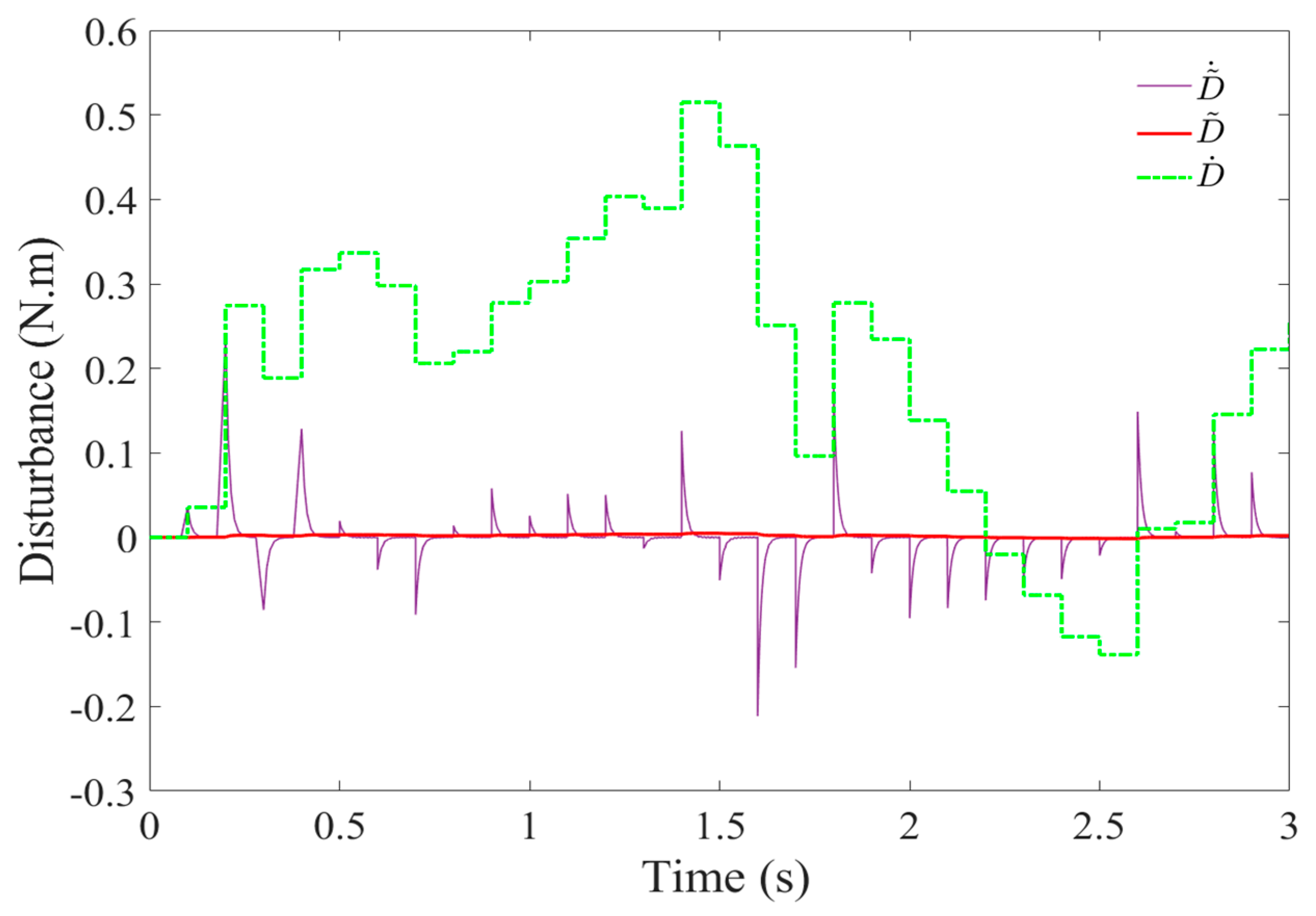
As illustrated in Figure 9, the error $\dot{\tilde{D}}\left(t\right)$ of the NSMO rapidly approaches 0 at the initial stage of the simulation and subsequently stabilizes. Concurrently, the error Equation (29), $\tilde{D}\left(t\right)$, exhibits fluctuations around 0, attributable to the impact of the input disturbance signal $D\left(t\right)$. Notably, the first-order derivative of the NSMO is constrained at the commencement of the simulation period. Additionally, Figure 9 demonstrates that the first-order derivative $\dot{D}\left(t\right)$ of the interfering signal $D\left(t\right)$ remains within certain limits during the simulation time, thereby validating the practicality of the NSMO and nonlinear function $g\left(S_{\mathrm{w}}\right)$ design.

3.3.2. Designing μ₁,μ₂ Parameter-Adaptive Law

In the absence of consideration of the filter design ($\widehat{\beta }=\beta$) and the disturbance estimation design ($\widehat{D}=D$), integrating the equations listed in footnotes (13), (19), and (25) with respect to the derivative of Equation (23) results in

$$\begin{array}{cc}\hfill {\dot{V}}_3& =-\left(K_{\mathrm{w}}{S}_{\mathrm{w}}^2+K_{\mathrm{q}}{S}_{\mathrm{q}}^2+K_{\mathrm{d}}{S}_{\mathrm{d}}^2\right)+{\lambda }_1{S}_{\mathrm{w}}{\Delta }_{\mathrm{q}}-{\lambda }_1{S}_{\mathrm{w}}\tilde{\beta }+S_{\mathrm{w}}\tilde{D}+{\tilde{\mu }}_1{S}_{\mathrm{q}}{i}_{\mathrm{q}}+{\tilde{\mu }}_2{S}_{\mathrm{d}}{i}_{\mathrm{d}}\hfill \\ & =-\left(K_{\mathrm{w}}{S}_{\mathrm{w}}^2+K_{\mathrm{q}}{S}_{\mathrm{q}}^2+K_{\mathrm{d}}{S}_{\mathrm{d}}^2\right)+{\lambda }_1{S}_{\mathrm{w}}{\Delta }_{\mathrm{q}}+{\tilde{\mu }}_1{S}_{\mathrm{q}}{i}_{\mathrm{q}}+{\tilde{\mu }}_2{S}_{\mathrm{d}}{i}_{\mathrm{d}}\hfill \end{array}$$

(35)

where ${\tilde{\mu }}_1$ is an error of ${\mu }_1, {\tilde{\mu }}_1=\mu -{\widehat{\mu }}_1\begin{array}{cc}.& {\tilde{\mu }}_2\end{array}$, which is an error of ${\mu }_2, {\tilde{\mu }}_2={\mu }_2-{\widehat{\mu }}_2.$ The adaptive law for parameter $\mu =\left[\begin{array}{l}{\mu }_1\\ {\mu }_2\end{array}\right]$ is designed as shown in Equation (36).

$$\dot{\widehat{\mu }}=\Pi \left(\left[\begin{array}{cc}{i}_{\mathrm{q}}& 0\\ 0& i_{\mathrm{d}}\end{array}\right]\left[\begin{array}{cc}{S}_{\mathrm{q}}& 0\\ 0& S_{\mathrm{d}}\end{array}\right]-\Sigma \left[\begin{array}{c}{\widehat{\mu }}_1\\ {\widehat{\mu }}_2\end{array}\right]\right)$$

(36)

where $\mathit{\Pi }, \mathit{\Sigma }$ are symmetric positive definite matrices. $\mathit{\Pi }=\left[\begin{array}{cc}{\varpi }_1& 0\\ 0& {\varpi }_2\end{array}\right],$ and $\mathit{\Sigma }=\left[\begin{array}{cc}{\epsilon }_1& 0\\ 0& {\epsilon }_2\end{array}\right]$, wherein ${\varpi }_1, {\varpi }_2, {\epsilon }_1$ and ${\epsilon }_2$ are all positive constants, and $\varpi ={\varpi }_1={\varpi }_2, \epsilon ={\epsilon }_1={\epsilon }_2$.

As illustrated in Figure 2, Equations (28) and (36) demonstrate a clear relationship between an increase in the external perturbation of the system and the subsequent effect on the system output w. This, in turn, exerts an influence on the input of the motor d-q-axis voltages, thereby inducing parametric instability in the motor. The development of an adaptive law (UPAL) to counteract system instability due to variations in motor current and voltage, resulting from disturbances, constitutes a pivotal approach to ensure operational stability and reliability.

It is imperative to consider the Lyapunov candidate function $V_5=V_3+V_{\mu }$ in Equation (37), wherein $V_{\mu }={\displaystyle \frac{1}{2\varpi }}{{\tilde{\mu }}_1}^2+{\displaystyle \frac{1}{2\varpi }}{{\tilde{\mu }}_2}^2$.

$$V_5=V_3+{\displaystyle \frac{1}{2\varpi }}\left({{\tilde{\mu }}_1}^2+{{\tilde{\mu }}_2}^2\right)$$

(37)

The derivation of $V_5$ is shown in Equation (38).

$${\dot{V}}_5={\dot{V}}_{\mathrm{w}}+{\dot{V}}_{\mathrm{q}}+{\dot{V}}_{\mathrm{d}}+{\displaystyle \frac{1}{\varpi }}\left({\tilde{\mu }}_1{\dot{\tilde{\mu }}}_1+{\tilde{\mu }}_2{\dot{\tilde{\mu }}}_2\right)$$

(38)

The application of $\widehat{\mu }=\left[\begin{array}{c}{\widehat{\mu }}_1\\ {\widehat{\mu }}_2\end{array}\right]$ to Equation (38) results in Equation (39).

$$\begin{array}{cc}\hfill {\dot{V}}_5& =-\left(K_{\mathrm{w}}{S}_{\mathrm{w}}^2+K_{\mathrm{q}}{S}_{\mathrm{q}}^2+K_{\mathrm{d}}{S}_{\mathrm{d}}^2\right)+{\lambda }_1{S}_{\mathrm{w}}{\Delta }_{\mathrm{q}}-{\displaystyle \frac{\epsilon }{\varpi }}\left({\tilde{\mu }}_1{\widehat{\mu }}_1+{\tilde{\mu }}_2{\widehat{\mu }}_2\right)\hfill \\ & =-\left(K_{\mathrm{w}}{S}_{\mathrm{w}}^2+K_{\mathrm{q}}{S}_{\mathrm{q}}^2+K_{\mathrm{d}}{S}_{\mathrm{d}}^2\right)+{\lambda }_1{S}_{\mathrm{w}}{\Delta }_{\mathrm{q}}-{\displaystyle \frac{\epsilon }{\varpi }}\left({\tilde{\mu }}_1^2+{\tilde{\mu }}_2^2+{\tilde{\mu }}_1{\mu }_1+{\tilde{\mu }}_2{\mu }_2\right)\hfill \\ & \le -\left(K_{\mathrm{w}}{S}_{\mathrm{w}}^2+K_{\mathrm{q}}{S}_{\mathrm{q}}^2+K_{\mathrm{d}}{S}_{\mathrm{d}}^2\right)+{\lambda }_1{S}_{\mathrm{w}}{\Delta }_{\mathrm{q}}-{\displaystyle \frac{\epsilon }{2\varpi }}\left({‖{\tilde{\mu }}_1‖}^2+{‖{\tilde{\mu }}_2‖}^2\right)+{\displaystyle \frac{\epsilon }{2\varpi }}\left({‖{\mu }_1‖}^2+{‖{\mu }_2‖}^2\right)\hfill \\ & \le -2\left(K_{\mathrm{w}}-{\lambda }_1\right)V_{\mathrm{w}}-2\left(K_{\mathrm{q}}-{\displaystyle \frac{{\lambda }_1}{2}}\right)V_{\mathrm{q}}-2K_{\mathrm{d}}{V}_{\mathrm{d}}-2\epsilon V_{\mu }+{\displaystyle \frac{{\lambda }_1}{2}}{\Delta }_{\mathrm{q}}^2\left(0\right)e^{-2{\gamma }_{\mathrm{q}}\mathrm{t}}+{\displaystyle \frac{\epsilon }{2\varpi }}\left({‖{\mu }_1‖}^2+{‖{\mu }_2‖}^2\right)\hfill \\ & \le -2{\varphi }_5{V}_5+C_5\hfill \end{array}$$

(39)

where ${\varphi }_5=\min \left\{K_{\mathrm{w}}-{\lambda }_1, K_{\mathrm{q}}-{\displaystyle \frac{{\lambda }_1}{2}}, K_{\mathrm{d}}, \epsilon \right\}, C_5={\displaystyle \frac{{\lambda }_1}{2}}{\Delta }_{\mathrm{q}}^2\left(0\right)e^{-2{\gamma }_{\mathrm{q}}\mathrm{t}}+{\displaystyle \frac{\epsilon }{2\varpi }}\left({‖{\mu }_1‖}^2+{‖{\mu }_2‖}^2\right)$.

It is evident that an identical analytical process to that delineated in Equation (14) results in the derivation of in Equation (40).

$$0\le V_5\left(t\right)\le {\varphi }_5+\left(V_5\left(0\right)-{\varphi }_5\right)e^{-2{\varphi }_{5}t}, \forall t\ge 0$$

(40)

A thorough examination of Equation (40) reveals a limitation of $V_5\left(t\right)$ by ${\varphi }_5$. Consequently, it can be deduced that ${\tilde{\mu }}_1, {\tilde{\mu }}_2$ are bounded. This indicates that the system can be ensured to be globally exponentially stable, and the parameter error ${\tilde{\mu }}_1, {\tilde{\mu }}_2$ can converge to zero in a finite time.

4. Stability Proof

For the purposes of facilitating the proof and analysis, the following assumptions are posited with respect to the desired trajectory w_ref(t):

Assumption 1.

The requisite reference input trajectories w_ref(t) and their derivatives ${\displaystyle \frac{d^{\left(j\right)}{w}_{\mathrm{ref}}\left(t\right)}{d^{j}t}}, \left(1\le j\le n\right)$ are bounded, continuous, and known.

Assumption 2.

The disturbances $D\left(t\right)$ and their first-order derivatives ${\displaystyle \frac{dD\left(t\right)}{dt}}$ in the system are bounded, continuous, and differentiable, and have $\left|\dot{D}\right|\le \Upsilon , \Upsilon$ positive constants.

Assumption 3.

The designed composite filters $\widehat{\beta }\left(t\right)$ and their derivatives ${\displaystyle \frac{d^{\left(j\right)}\widehat{\beta }\left(t\right)}{d^{j}t}}, \left(1\le j\le n\right)$ are known to be bounded, continuous, and well defined.

In an analysis of the stability of a specific nonlinear system, Lyapunov theory provides an effective method to solve the problem of nonlinear system stability that cannot be addressed by the stability criteria in classical control theory (e.g., algebraic criterion, Laws criterion, root-trajectory method, etc.). According to the Lyapunov theory of the energy stability of systems, all controllers in the entire control system, including the designed NSMO and UPAL, are taken into account. The stability of the AFTCFBC is thus proven and analyzed in detail.

The Lyapunov candidate function $V$ is selected in accordance with the specifications outlined in Equation (41).

$$V=V_{\mathrm{w}}+V_{\mathrm{q}}+V_{\mathrm{d}}+V_{\beta }+V_{\mathrm{D}}+V_{\mu }$$

(41)

The derivation of $V$ is shown in Equation (42).

$$\dot{V}=S_{\mathrm{w}}{\dot{S}}_{\mathrm{w}}+S_{\mathrm{q}}{\dot{S}}_{\mathrm{q}}+S_{\mathrm{d}}{\dot{S}}_{\mathrm{d}}+\tilde{\beta }\dot{\tilde{\beta }}+\tilde{D}\dot{\tilde{D}}+{\tilde{\mu }}_1{\dot{\tilde{\mu }}}_1+{\tilde{\mu }}_2{\dot{\tilde{\mu }}}_2$$

(42)

The result of combining the solutions to Equations (3), (7), (19), (25), (29) and (35) with Equation (42) is shown in in Equation (43).

$$\begin{array}{cc}\hfill \dot{V}& =-K_{\mathrm{w}}{S}_{\mathrm{w}}^2-K_{\mathrm{q}}{S}_{\mathrm{q}}^2-K_{\mathrm{d}}{S}_{\mathrm{d}}^2+{\lambda }_1{S}_{\mathrm{w}}{\Delta }_{\mathrm{q}}-{\lambda }_1{S}_{\mathrm{w}}\tilde{\beta }+S_{\mathrm{w}}\tilde{D}+{\dot{V}}_{\mathrm{D}}-{\displaystyle \frac{\epsilon }{\varpi }}\left({\tilde{\mu }}_1{\widehat{\mu }}_1+{\tilde{\mu }}_2{\widehat{\mu }}_2\right)\hfill \\ & =-K_{\mathrm{w}}{S}_{\mathrm{w}}^2-K_{\mathrm{q}}{S}_{\mathrm{q}}^2-K_{\mathrm{d}}{S}_{\mathrm{d}}^2+{\lambda }_1{S}_{\mathrm{w}}{\Delta }_{\mathrm{q}}^2\left(0\right)e^{-2{\gamma }_{\mathrm{q}}\mathrm{t}}+{\lambda }_1{S}_{\mathrm{w}}{S}_{\mathrm{q}}+{\lambda }_1{S}_{\mathrm{w}}\tilde{\beta }+S_{\mathrm{w}}\tilde{D}+\hfill \\ & {\dot{V}}_{\beta }+\tilde{D}\dot{\tilde{D}}-{\displaystyle \frac{\epsilon }{\varpi }}\left({\tilde{\mu }}_1{\widehat{\mu }}_1+{\tilde{\mu }}_2{\widehat{\mu }}_2\right)\hfill \end{array}$$

(43)

The simplified Equation (43), derived from the premises of Lemma 1, is thus written as in Equation (46).

$$\begin{array}{cc}\hfill \dot{V}& ={\dot{V}}_{\beta }-K_{\mathrm{w}}{S}_{\mathrm{w}}^2-K_{\mathrm{q}}{S}_{\mathrm{q}}^2-K_{\mathrm{d}}{S}_{\mathrm{d}}^2+{\lambda }_1{S}_{\mathrm{w}}{\Delta }_{\mathrm{q}}\left(0\right)e^{-{\gamma }_{\mathrm{q}}\mathrm{t}}+{\lambda }_1{S}_{\mathrm{w}}{S}_{\mathrm{q}}-{\lambda }_1{S}_{\mathrm{w}}\tilde{\beta }+S_{\mathrm{w}}\tilde{D}+\hfill \\ & \tilde{D}\left(-g\left(S_{\mathrm{w}}\right)\tilde{D}-\dot{D}\right)-{\displaystyle \frac{\epsilon }{\varpi }}\left({\tilde{\mu }}_1{\widehat{\mu }}_1+{\tilde{\mu }}_2{\widehat{\mu }}_2\right)\hfill \\ & \le -K_{\mathrm{w}}{S}_{\mathrm{w}}^2-K_{\mathrm{q}}{S}_{\mathrm{q}}^2-K_{\mathrm{d}}{S}_{\mathrm{d}}^2+{\displaystyle \frac{{\lambda }_1}{2}}{S}_{\mathrm{w}}^2+{\displaystyle \frac{{\lambda }_1}{2}}{\Delta }_{\mathrm{q}}^2\left(0\right)e^{-2{\gamma }_{\mathrm{q}}\mathrm{t}}+{\displaystyle \frac{{\lambda }_1}{2}}{S}_{\mathrm{w}}^2+{\displaystyle \frac{{\lambda }_1}{2}}{S}_{\mathrm{q}}^2+{\displaystyle \frac{{\lambda }_1}{2}}{S}_{\mathrm{w}}^2+{\displaystyle \frac{{\lambda }_1}{2}}{\tilde{\beta }}^2+\hfill \\ & {\displaystyle \frac{1}{2}}{S}_{\mathrm{w}}^2+{\displaystyle \frac{1}{2}}{\tilde{D}}^2-g\left(S_{\mathrm{w}}\right){\tilde{D}}^2+{\displaystyle \frac{1}{2}}{\tilde{D}}^2+{\displaystyle \frac{1}{2}}{\Upsilon }^2-{\displaystyle \frac{\epsilon }{\varpi }}\left({\tilde{\mu }}_1{\widehat{\mu }}_1+{\tilde{\mu }}_2{\widehat{\mu }}_2\right)+{\dot{V}}_{\beta }\hfill \\ & \le -\left(K_{\mathrm{w}}-{\displaystyle \frac{3{\lambda }_1}{2}}-{\displaystyle \frac{1}{2}}\right)S_{\mathrm{w}}^2-\left(K_{\mathrm{q}}-{\displaystyle \frac{{\lambda }_1}{2}}\right)S_{\mathrm{q}}^2-K_{\mathrm{d}}{S}_{\mathrm{d}}^2-\left(m-{\displaystyle \frac{{\lambda }_1}{2}}\right){\tilde{\beta }}^2-2\left(G_{\min }-1\right){\tilde{D}}^2-\hfill \\ & 2\epsilon V_{\mu }+{\displaystyle \frac{{\dot{D}}^2}{2}}+{\displaystyle \frac{{\lambda }_1}{2}}{\Delta }_{\mathrm{q}}^2\left(0\right)e^{-2{\gamma }_{\mathrm{q}}\mathrm{t}}+{\displaystyle \frac{\epsilon }{2\varpi }}\left({‖{\mu }_1‖}^2+{‖{\mu }_2‖}^2\right)\hfill \end{array}$$

(44)

Ultimately, the simplification is represented by Equation (45).

$$\begin{array}{cc}\hfill \dot{V}& \le -2\left(K_{\mathrm{w}}-{\displaystyle \frac{3{\lambda }_1}{2}}-{\displaystyle \frac{1}{2}}\right)V_{\mathrm{w}}-2\left(K_{\mathrm{q}}-{\displaystyle \frac{{\lambda }_1}{2}}\right)V_{\mathrm{q}}-2K_{\mathrm{d}}{V}_{\mathrm{d}}-2\left(m-{\displaystyle \frac{{\lambda }_1}{2}}\right)V_{\beta }-2\epsilon V_{\mu }\hfill \\ & -2\left(G_{\min }-1\right)V_{\mathrm{D}}+{\displaystyle \frac{\epsilon }{2\varpi }}{‖{\mu }_1‖}^2+{\displaystyle \frac{\epsilon }{2\varpi }}{‖{\mu }_2‖}^2+{\displaystyle \frac{1}{2}}{\Upsilon }^2+{\displaystyle \frac{{\lambda }_1^2}{2}}{\Delta }_{\mathrm{q}}^2\left(0\right)e^{{-2\gamma }_{\mathrm{q}}\mathrm{t}}\hfill \\ & \le -2\varphi V+C\hfill \end{array}$$

(45)

where $\varphi , C$ are constant, with $\varphi =\min \left\{K_{\mathrm{w}}-{\displaystyle \frac{3{\lambda }_1}{2}}-{\displaystyle \frac{1}{2}}, K_{\mathrm{q}}-{\displaystyle \frac{{\lambda }_1}{2}}, K_{\mathrm{d}}, m-{\displaystyle \frac{{\lambda }_1}{2}}, \epsilon , G_{\min }-1\right\}$ and $C={\displaystyle \frac{{\Upsilon }^2}{2}}+{\displaystyle \frac{{\lambda }_1}{2}}{\Delta }_{\mathrm{q}}^2\left(0\right)e^{-2{\gamma }_{\mathrm{q}}\mathrm{t}}+{\displaystyle \frac{\epsilon }{2\varpi }}{‖{\mu }_1‖}^2+{\displaystyle \frac{\epsilon }{2\varpi }}{‖{\mu }_2‖}^2$.

Upon analysis of the aforementioned integral Equation (45), it becomes evident that if $\varphi >{\displaystyle \frac{C}{2\tau }}\left(\tau >0\right)$, when $V=\tau , \dot{V}\le -2\varphi \tau +C$, there is $\dot{V}\le 0$. This signifies that $\dot{V}\le \tau$ is an invariant set $V\left(t\right)\le \tau \left(t\ge 0\right)$ with respect to $V=\tau$, as illustrated in Equation (46).

$$0\le V\left(t\right)\le \varphi +\left(V\left(0\right)-\varphi \right)e^{-2\varphi t}, \forall t\ge 0$$

(46)

It is evident that V(t) is subject to the constraint ϕ. This observation leads to the conclusion that $S_{\mathrm{w}}, S_{\mathrm{q}}, S_{\mathrm{q}}, {\tilde{\mu }}_1, {\tilde{\mu }}_2$ and $\tilde{D}$ are bounded. When this result is considered in conjunction with the finite-time stability theorem for nonlinear systems, it becomes evident that system (2) is finite-time-stable in the designed controller.

5. Simulation

In order to simulate the performance of the ship in the actual sailing process, this study employs a model of a PMSM based on the theory of the AFTCFBC within the MATLAB/Simulink environment, subsequently undertaking a verification process through simulation. In consideration of the operational characteristics of ships in disparate marine environments, the simulation analysis of the PMSM is divided into four typical working conditions. In order to further validate the feasibility and superiority of the proposed control method and its theory, the present study compares the performance of Adaptive Backstepping Sliding Mode Controller (ABSMC), Command-Filtered Backstepping Sliding Mode Controller (CFBSMC), and conventional proportional–integral (PI) control strategies under these operating conditions. In particular, both the ABSMC and CFBSMC control algorithms mentioned in the simulations are designed within the framework of the control theory proposed in this paper. The ABSMC algorithm is designed without an NFTCF, while the CFBSMC algorithm is designed without the UPAL.

5.1. Data Preparation

This section presents a comprehensive list of the motor parameters employed in the simulation process of this study, along with the pertinent control parameters of the aforementioned four controllers. These parameters are crucial for ensuring the efficacy of the designed control strategy and the reliability of the simulation results. For detailed information, please refer to

Table 1. The parameters required for the simulation of a PMSM.

Parameters	Value
Pole pairs Pn	4
Stator resistance Rs/Ω	0.958
Winding resistance Ls/mH	5.25
Moment of inertia J/(kg.m2)	0.0000003
Viscous damping factor B	0.003
Rotor magnetic chain Ψf/Wb	0.1827
Rated voltage/V	540
Rated speed/rpm	750

and

Table 2. The parameters required for the simulation of different controllers.

Controller	Controller Parameters
	Rotating Speed Loop	Current Loop
AFTCFBC	$\begin{array}{l}r=0.5, \rho =0.02, l=10;\\ K_{\mathrm{w}}={1.1}^{\ast }B/J, K_{\mathrm{q}}={ 1.8}^{\ast }B/J, K_{\mathrm{d}}={ 0.4}^{\ast }B/J;\\ {\gamma }_{\mathrm{w}}=120, {\gamma }_{\mathrm{q}}= 40, {\gamma }_{\mathrm{d}}=20;\\ {\varpi }_1=0.3, {\varpi }_2=0.3, {\epsilon }_1=0.2, {\epsilon }_2=0.2.\end{array}$

.

5.2. Multi-Case Simulation for Comparative Verification

5.2.1. Condition 1—Constant Speed and Constant Torque

The motor is set at a constant speed of 500 r/min and a constant torque of 10 N·m, which is typical for operational processes where the ship requires stability in speed and propulsion. This is exemplified by situations where the ship sails for an extended period or needs to maintain a specific working point. The simulation results are presented in Figure 10 for the purposes of illustration.

In Figure 10a,b, it can be observed that the rotor speed of all four controllers can be rapidly tracked to the specified reference speed input, and that the dynamic and steady-state performance of the system aligns with the control requirements. In comparison to the PI control, the three controllers, ABSMC, CFBSMC, and AFTCFBC, demonstrate a notable absence of overshooting, a markedly enhanced response speed, a considerably reduced maximum steady-state error, and a diminished level of jitter.

As illustrated in

Table 3. Indicator elements of rotational speed with different controllers.

Performance	AFTCFBC	CFBSMC	ABSMC	PI
Overshoot	0	0	0	6.44%
Response time (s)	0.105	0.105	1.131	0.129
Maximum steady-state error (r/min)	0.50	0.50	0.80	1.70
Intermittent oscillation peak-to-peak value (r/min)	0.959	0.962	0.922	2.892

, which presents the rotor speed characteristics with the four controllers, the response time of the AFTCFBC is reduced by 18.6% in comparison with PI. The integral squared error of PI is 1.83744, whereas that of the AFTCFBC is 0.180938, which is reduced by 90.15% in comparison with PI. Furthermore, the maximum steady-state error of the AFTCFBC and CFBSMC speeds in the stable operation phase is 0.5, representing a 37.5% reduction in comparison to the ABSMC. The peak-to-peak value of the steady-state jitter of the AFTCFBC is reduced by 70.6% in comparison to the PI control, while the CFBSMC reduction is 0.3% and the PI reduction is 66.8%. The peak-to-peak value of the steady-state jitter of the ABSMC is reduced by 68.1% in comparison to the PI control. The data from this study demonstrate that the AFTCFBC exhibits a comparatively superior control effect. It can be observed that the combined control performance of the AFTCFBC is the most effective among the four control methods.

As illustrated in Figure 10c and

Table 4. Indicator elements of torque with different controllers.

Performance	AFTCFBC	CFBSMC	ABSMC	PI
Overshoot	7.3%	7.3%	16.2%	121.4%
Response time (s)	0.054	0.054	0.054	0.039
Maximum steady-state error (r/min)	0.96	0.95	0.96	1.27
Intermittent oscillation peak-to-peak value (r/min)	1.809	1.792	1.804	2.446

, all four controllers demonstrate the capacity to rapidly attain the specified reference torque input. In comparison to the PI control, the three controllers, ABSMC, CFBSMC, and AFTCFBC, demonstrate a reduction in overshoot, maximum steady-state error, and jitter. In particular, the PI control is outperformed by the AFTCFBC in terms of overshoot, maximum steady-state error, and jitter peak-to-peak value, with reductions of 94.0%, 24.4%, and 26.0%, respectively. This evidence substantiates the AFTCFBC’s superior performance in both steady-state and dynamic operations.

A comparison of the design of the CFBSMC and AFTCFBC reveals a notable distinction. The former does not incorporate the UPAL module, which plays a pivotal role in estimating uncertainty parameters within the system. Consequently, the overall gain function is primarily influenced by the sliding mode function and the interference D. This observation underscores the similarity in the control behavior of the two controllers, AFTCFBC and CFBSMC.

Figure 10d clearly shows that the three controllers, ABSMC, CFBSMC, and AFTCFBC, exhibit a comparable disturbance estimation effect, exhibiting fluctuations of approximately $-3.27\times {10}^7$ N·m when the motor is operating smoothly. The precision of disturbance estimation directly influences the magnitude of the cross-axis virtual control current, which can most effectively compensate for the unpredictability of the motor torque output.

In the context of condition 1, characterized by constant speed and constant torque, the simulation study advances based on the control block diagram depicted in Figure 2. This approach enables the acquisition of the main state values of each component, including the SVPMW waveforms, three-phase voltages $u_{\mathrm{abc}}$, the rotor position θ, the d-q-axis currents, and three-phase currents, of the PMSM with the AFTCFBC. The outcomes of this study are illustrated in Figure 11, Figure 12, Figure 13 and Figure 14.

As demonstrated in Figure 11, the SVPMW waveform of the PMSM under the influence of the AFTCFBC exhibits stable and regular characteristics; the six switching signals output from SVPWM to the inverter (denoted by S₁, S₂, S₃, S₄, S₅, and S₆) are shown in Figure 2.

Figure 12 clearly shows that the amplitude and phase of the three-phase voltage $u_{\mathrm{abc}}$ are relatively stable. As illustrated in Figure 13, the rotor position θ is updated with precision in real time, indicating the PMSM’s capacity for stable operation and precise control with the AFTCFBC. The efficacy of the method is evident, underscoring its feasibility.

The rotor position θ in Figure 13 is obtained by employing Vector Control (VC), subsequent to coordinate transformation (e.g., Clarke transformation, Park transformation), which converts the three-phase stator currents to the synchronous rotating coordinate system. Thereafter, the rotor position can be derived according to the relationship between the active and reactive components of the currents and the rotor position. Additionally, the Direct Torque Method (DTC) can be employed to derive the rotor position. This method involves measuring the stator voltage and current, calculating the stator magnetic chain, and subsequently deriving the rotor position based on the relationship between the stator magnetic chain and the rotor position.

As evidenced by Figure 14, the dq-axis current waveform is stable, with $i_{\mathrm{d}}$ exhibiting fluctuations at 0, while $i_{\mathrm{q}}$ remains stable at approximately 10 A. Concurrently, the three-phase current $i_{\mathrm{abc}}$ is symmetrical and exhibits no substantial harmonics, thereby validating the efficacy of the AFTCFBC in achieving precise current control and ensuring the stability of motor torque output under operating condition 1. This outcome is pivotal in guaranteeing the efficient operation and reliable performance of the system.

5.2.2. Condition 2—Variable Speed and Constant Torque

The motor is set to operate at a constant speed of 500 r/min and a constant torque of 10 N·m. The motor rotor speed rises to 600 r/min in one second and falls to 400 r/min in two seconds. This phenomenon can be observed in operational scenarios where the ship requires a change in the speed and stabilization of the propulsion system, such as during sailing and docking maneuvers. The results of the motor simulation are presented in Figure 15.

As illustrated in Figure 15a,b, all four controller rotor speeds are capable of being rapidly tracked to a specified reference speed input following a 1 s ramp-up of 100 r/min and a 2 s ramp-down of 200 r/min. In comparison to the PI control, the three controllers (ABSMC, CFBSMC, and AFTCFBC) demonstrate superior tracking capabilities to the reference input, exhibiting reduced overshoot and jitter control following a rotor speed-up or -down.

Figure 15c illustrates that the three controllers, ABSMC, CFBSMC, and AFTCFBC, rapidly converge on the desired value of the reference input torque following the lifting and lowering of the motor, exhibiting superior stability compared to the PI control. A comparison of Figure 10d and Figure 15d demonstrates that the disturbance estimation is subject to variation in accordance with rotor speed, exhibiting a positive correlation.

As demonstrated in Figure 16, under condition 2 of variable speed with constant torque, the dq-axis current waveform is stable. The current i_d increases convexly when the speed is raised and lowered at time 1 s, and concavely when the speed is lowered at time 2 s. Concurrently, the three-phase current $i_{\mathrm{abc}}$ is also stable and symmetrical without significant harmonics, thereby demonstrating that the AFTCFBC can achieve accurate current control and the stability of motor rotor speed output under condition 2.

5.2.3. Condition 3—Constant Speed and Step Torque

The motor is set to perform load and unload simulations under a constant speed of 500 r/min and a constant load torque of 10 N·m. This is carried out in order to verify the dynamic response and stability performance of the motor. A load of 15 N·m is applied for a period of one second, after which an unloading of 5 N·m is initiated and maintained for a further two seconds. This operational process is representative of the methods typically employed by ships to stabilize their speed and alter their propulsive force, for instance, in the event of a sudden storm at sea. The results of the motor simulation are presented in Figure 17.

As illustrated in Figure 17a,b, all four controller speeds demonstrate the capacity to be rapidly tracked to a specified reference speed input following a one-second loading period of 15 N·m and a two-second unloading period of 5 N·m. Moreover, the four controllers display a superior capacity to track the reference speed input in comparison to the PI control. In comparison to the PI control, the three controllers, ABSMC, CFBSMC, and AFTCFBC, demonstrate enhanced tracking capabilities to the reference input, both during loading and unloading. This is evidenced by the reduction in error and jitter control, coupled with the absence of oscillation following loading and unloading.

Figure 17c illustrates that the three controllers, ABSMC, CFBSMC, and AFTCFBC, demonstrate the rapid tracking of the desired value of the reference input torque following the loading or unloading of the motor. Their stability performance is superior to that of the PI control. In Figure 10d and Figure 17d, it can be observed that the disturbance estimation is more responsive to changes in torque than to changes in rotational speed. Furthermore, there is a positive correlation between the two variables in terms of numerical changes.

As demonstrated in Figure 18, under condition 3 of constant speed and variable torque, the dq-axis current waveform exhibits stability. A sudden increase in the current i_d is observed at time 1 s, followed by a subsequent decrease at time 2 s, coinciding with a reduction in load. Concurrently, the three-phase current i_abc is observed to be stable and symmetrical, devoid of significant harmonics. This outcome serves to substantiate the efficacy of the AFTCFBC in attaining precise current control and ensuring the stability of the motor torque output under condition 3.

5.2.4. Condition 4—Variable Speed and White Noise Torque

The motor is set to perform a stochastic white noise speed-lift simulation at a constant speed of 500 r/min and a constant load torque of 10 N·m. This is carried out in order to verify the motor’s dynamic response and stability performance. The motor speed is then ramped up to 600 r/min. The motor speed is then reduced to 400 r/min over a period of 2 s. This configuration is representative of operational scenarios that necessitate concurrent adjustments in speed and propulsion, such as a ship encountering an unforeseen event in open waters. The outcomes of the motor simulation are illustrated in Figure 19.

As illustrated in Figure 19a,b, even when subjected to white noise perturbations, the four controller speeds can still be rapidly tracked to a specified reference speed after a one-second ramp-up of 100 r/min and a two-second ramp-down of 200 r/min. In comparison to the PI control, the three controllers, ABSMC, CFBSMC, and AFTCFBC, demonstrate superior performance in tracking the ramp-up and ramp-down speeds in the presence of white noise perturbations, thereby enhancing the control effect. As shown in Figure 19c,d, in the presence of white noise disturbances, the three controllers, ABSMC, CFBSMC, and AFTCFBC, are capable of tracking the reference torque input intermittently and exhibit superior stability compared to the PI control. In the presence of disturbances and uncertain parameter inputs from the external environment, the AFTCFBC is capable of rapid compensation and response output through the estimation of the disturbances via the NSMO.

As demonstrated in Figure 20, under the condition of variable-speed white noise torque, the dq-axis current wave demonstrates a dynamic relationship with the input white noise torque. Concurrently, the three-phase current i_abc exhibits a synchronized response, mirroring the fluctuations in the white noise torque. This observation unveils the symmetrical and non-significant harmonic characteristics of the system, thereby substantiating the efficacy of the AFTCFBC in attaining precise current control and ensuring the stability of motor speed and torque output under condition 4.

In conclusion, the NSMO-based ABSMC, CFBSMC, and AFTCFBC proposed in this paper can be applied to the control of ship propulsion motors. They are capable of adapting to unknown perturbations in the external environment and changes in their own parameters while improving their dynamic and steady-state performances. Consequently, the PMSM is able to meet the driving requirements of the ship under different sea conditions.

6. Conclusions

The issue of rotational speed oscillation and overshoot in the PMSM system of a new energy hybrid ship propulsion system, attributed to load variation and parameter uncertainty, is addressed in this paper. The speed control algorithm of the AFTCFBC based on NSMO, as proposed in this paper, integrates backstepping control, sliding mode control, adaptive control, and finite-time control to effectively mitigate the impact of unknown load perturbations stemming from changes in the external marine environment. The specific conclusions are as follows:

(1)

The NFTCF has been designed in such a way that the computational complexity issues associated with conventional backstepping control are effectively negated. Furthermore, the maximum steady-state error of the motor output speed has been reduced, and the overall stability of the control system has been enhanced.

(2)

The estimation of input load torque compensation in the new energy ship PMSM system is achieved by the NSMO and UPAL, which markedly enhances the dynamic performance of the ship propulsion system and the anti-disturbance capability of the load, while concurrently reducing the additional energy consumption of the system. This facilitates the safe and seamless operation of the ship electric propulsion system in diverse marine environments.

(3)

In comparison to the conventional PI control methodology, the AFTCFBC approach demonstrates a notable reduction in overshoot in speed tracking, with a 100% elimination of overshoot in some cases. Additionally, the AFTCFBC exhibits an 18.6% reduction in response time, a 37.5% reduction in maximum steady-state error, and a 66.8% reduction in the peak-to-peak value of steady-state jitter. Furthermore, the peak-to-peak value of steady-state jitter of the AFTCFBC is reduced by 0.3% in comparison to the CFBSMC. Additionally, the AFTCFBC demonstrates a notable reduction in the magnitude of overshoot in torque tracking in comparison to the ABSMC, resulting in optimal combined motor speed and torque control performance.

(4)

Three advanced motor controllers have been proposed in this paper; the CFBSMC, ABSMC, and AFTCFBC have been simulated and verified, and the AFTCFBC combines the advantages of both the CFBSM and ABSMC control technologies. All three controllers are able to meet the speed and torque control requirements of the PMSM in new energy hybrid ships under variable sea conditions, thereby confirming the significant advantages of the control strategy in improving motor efficiency, reducing energy consumption, and enhancing system robustness, as well as in achieving precise control of the PMSM.

In light of the considerable influence that complex and evolving meteorological circumstances exert on the actual navigation of ships, it seems prudent to consider the potential benefits of a data-driven AFTCFBC intelligent mathematical model that is grounded in real-time environmental variables in the future. The results of this study demonstrate a significant reduction in speed-tracking overshoot to zero, a substantial decrease in integral squared error by 90.15%, and a notable improvement in response time by 18.6%.