1. Introduction
The optimization algorithm is a mathematical technique for determining the optimal solution to a problem given constraints or limitations. In contemporary research, a wide range of disciplines, including prediction, control, and mechanical systems, employ optimization methodologies. Current research on optimization algorithms focuses on achieving optimal solutions with minimal computational time and resources while balancing global and local search capabilities. Early-stage optimization algorithms require significant computational resources and labor and suffer from issues such as overreliance on initial solutions and local minima stagnation [
1,
2]. Furthermore, most real-world models requiring optimization exhibit complex constraints, high-dimensional decision variables, and pronounced nonlinear properties, posing challenges for effective algorithmic solutions [
3,
4]. Consequently, researchers have proposed metaheuristic algorithms to address the complexity and computational challenges of optimization processes.
Typically, metaheuristic algorithms fall into three categories [
5]: evolution-based algorithms, physics-based algorithms, and population-based algorithms. Among these, evolution-based algorithms draw inspiration from natural evolution. The most prominent example is the Genetic Algorithm (GA), proposed by Holland in 1992, which implements Darwinian evolutionary theory [
6]. Physics-based algorithms emulate physical laws; the classic example is the Simulated Annealing Algorithm (SA), proposed by Kirkpatrick et al. in 1983 [
7]. SA models the metallurgical annealing process and probabilistically accepts suboptimal solutions to escape local optima. Currently, the most popular and rapidly evolving stochastic algorithms are population-based algorithms, which mimic collective behaviors in biological populations. Two classical examples are Particle Swarm Optimization (PSO) [
8] (Kennedy et al., 1995) and Ant Colony Optimization (ACO) [
9] (Dorigo et al., 2006). PSO simulates avian flocking behavior, while ACO emulates ant foraging strategies. Subsequent developments have produced algorithms such as the Krill Herd Algorithm (KH) [
10], Gray Wolf Optimization (GWO) [
11], the Whale Optimization Algorithm (WOA) [
12], Tuna Swarm Optimization (TSO) [
13], and Hippopotamus Optimization (HO) [
14]. These algorithms are valued for their model independence, gradient-free operation, robust global search capability, versatility, and computational efficiency [
15].
Most engineering problems require multi-objective rather than single-objective optimization. For example, an underwater manipulator operates as a multibody dynamic system that simultaneously requires optimization of joint kinematics, motion duration, energy consumption, and vibration suppression. In nonlinear multi-objective optimization, conflicting objectives often arise where some functions require maximization while others necessitate minimization. Unlike single-objective problems, the solution involves identifying Pareto-optimal solutions that represent the best achievable trade-offs between competing objectives. Consequently, developing robust multi-objective optimization algorithms constitutes the current research frontier in this field.
Currently, researchers primarily employ Pareto dominance and non-dominated sorting mechanisms to enhance single-objective optimization algorithms for multi-objective optimization. The most widely used algorithms include Multi-Objective Particle Swarm Optimization (MOPSO) [
16,
17], proposed by Coello et al., which integrates Pareto dominance into Particle Swarm Optimization (PSO) to handle multi-objective problems; the Non-Dominated Sorting Genetic Algorithm (NSGA) [
18], developed by Deb and Srinivas using non-dominated sorting to upgrade single-objective algorithms; NSGA-II [
19], an improved version by Deb et al. featuring a computationally efficient fast non-dominated sorting mechanism; other variant algorithms, such as Multi-Objective Gray Wolf Optimization (MOGWO) [
20], the Non-Dominated Sorting Whale Optimization Algorithm (NSWOA) [
21], the Multi-Objective Whale Optimization Algorithm (MOWOA) [
22], Non-Dominated Sorting Gray Wolf Optimization (NSGWO) [
23], the Multi-Objective Jellyfish Search Optimizer (MOJSO) [
24], and Multi-Objective Tuna Swarm Optimization (MOTSO) [
25]. However, existing multi-objective algorithms exhibit limitations in universal applicability. The No-Free-Lunch Theorem motivates researchers to develop novel metaheuristics or refine existing algorithms for domain-specific optimization challenges [
26].
At present, numerous researchers have optimized manipulator trajectories using multi-objective optimization algorithms. Huang et al. [
27] employed the Multi-Objective Particle Swarm Optimization (MOPSO) method to solve an objective function comprising motion time, dynamic perturbation, and acceleration, obtaining an efficient and safe motion trajectory for a space robot. Marcos et al. [
28] combined the closed-loop pseudo-inverse method with a Multi-Objective Genetic Algorithm (MOGA) to minimize joint displacements and end-effector position errors. Zhou et al. [
29] proposed a time-optimal trajectory planning method for manipulators based on an improved butterfly algorithm. Yang et al. [
30] developed a time-optimal trajectory planning method using the Marine Predators Algorithm (MPA) to satisfy the high-efficiency and high-precision operational requirements of manipulators. Additionally, other scholars have utilized and enhanced NSGA-II for manipulator trajectory optimization [
31,
32,
33,
34]. Due to the more complex working environments and the need to maintain stable and efficient operations, underwater manipulators face more challenging trajectory control compared to their land-based counterparts. Consequently, optimization outcomes for time, energy, and impact must meet stricter criteria. It is therefore insufficient to address underwater manipulators’ operational requirements by optimizing solely time or individual objective functions. The Tuna Swarm Optimization (TSO) algorithm exhibits rapid convergence, high solution accuracy, and excellent flexibility and scalability. It has been successfully applied to diverse optimization problems, including wind turbine fault classification [
35], autonomous underwater vehicle path planning [
36], Unmanned Aerial Vehicle (UAV) path planning [
37], and other domains with demonstrated efficacy.
Therefore, in this paper, the Fast Non-Dominated Sorting Tuna Swarm Optimization algorithm (FNS-TSO) is proposed by improving the TSO algorithm and is used to optimize the trajectory of an underwater manipulator. The main novel contributions of this study are as follows: 1. integrating the fast non-dominated sorting mechanism into the TSO algorithm; 2. improving the initialization of FNS-TSO by Optimal Latin Hypercube Sampling; 3. designing a nonlinear dynamic weight to improve the convergence and robustness of the FNS-TSO algorithm.
This paper is structured as follows:
Section 2 introduces the proposed FNS-TSO algorithm.
Section 3 presents a comparative analysis of the standard test function optimization results.
Section 4 demonstrates the algorithm’s application in underwater manipulator trajectory optimization.
Section 5 summarizes the key findings and provides actionable recommendations for future research.
2. Fast Non-Dominated Sorting Tuna Swarm Optimization (FNS-TSO)
The Tuna Swarm Optimization (TSO) algorithm is a new population-based metaheuristic optimization algorithm proposed by Xie et al. in 2021 [
13], based on modeling two foraging behaviors (spiral foraging and parabolic foraging) of tuna swarms. This section focuses on the improvements made to the TSO algorithm and does not provide a detailed description of the underlying algorithm.
2.1. Optimal Latin Hypercube Sampling Initialization Strategy
Latin Hypercubic Sampling (LHS) is a stratified sampling technique for approximate random sampling from multivariate parameter distributions, first proposed by McKay et al. [
38] and widely applied in multidisciplinary fields.
Following Mckay et al. in 1979 [
38], let
be a Latin hypercube of
runs for
factors that is a
matrix where each column is obtained as a uniform permutation on
and these columns are obtained independently. A
Latin hypercube design
based on
is generated through [
38]:
Specific explanations are provided in
Appendix A.1.
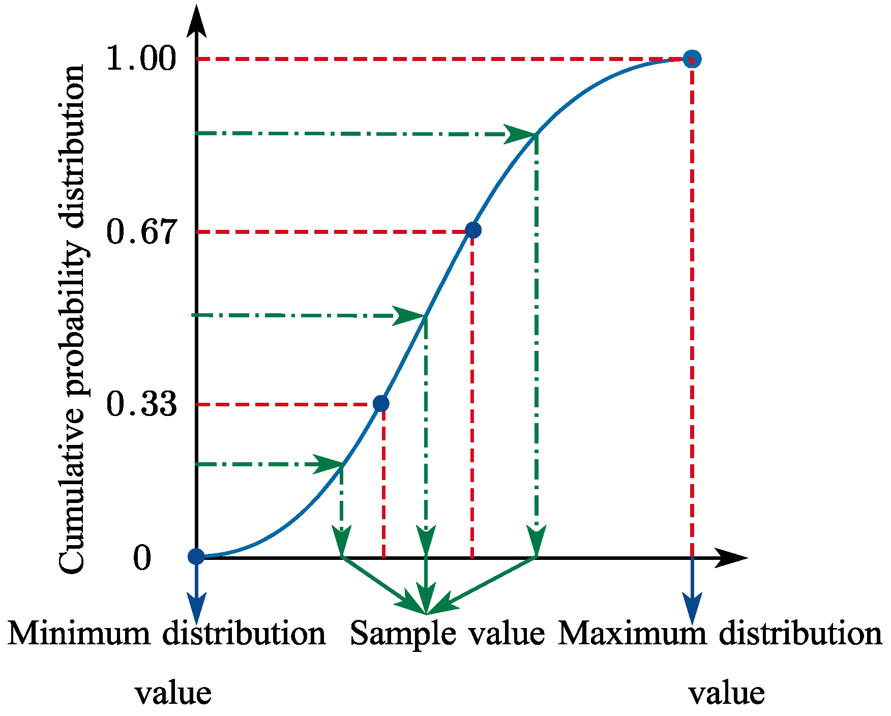
Stratifying the input probability distribution is fundamental to Latin Hypercube Sampling. On the cumulative probability scale (0 to 1.0), this method divides the cumulative distribution curve into equal intervals. A random sample is then selected from each stratum (or interval) of the input distribution.
The cumulative probability distribution function curve is separated into three intervals, as illustrated in
Figure 1. One sample is drawn from each interval, and the interval is excluded from subsequent sampling once sampled. In practical applications, this approach proves efficient because the samples can more accurately reflect input probability distributions, avoiding the “clustering” phenomenon that may occur with small sample sizes.
The optimal design used in this paper is called a maximin distance design if it maximizes the minimum inter-site distance [
39]:
Specific explanations are provided in
Appendix A.1.
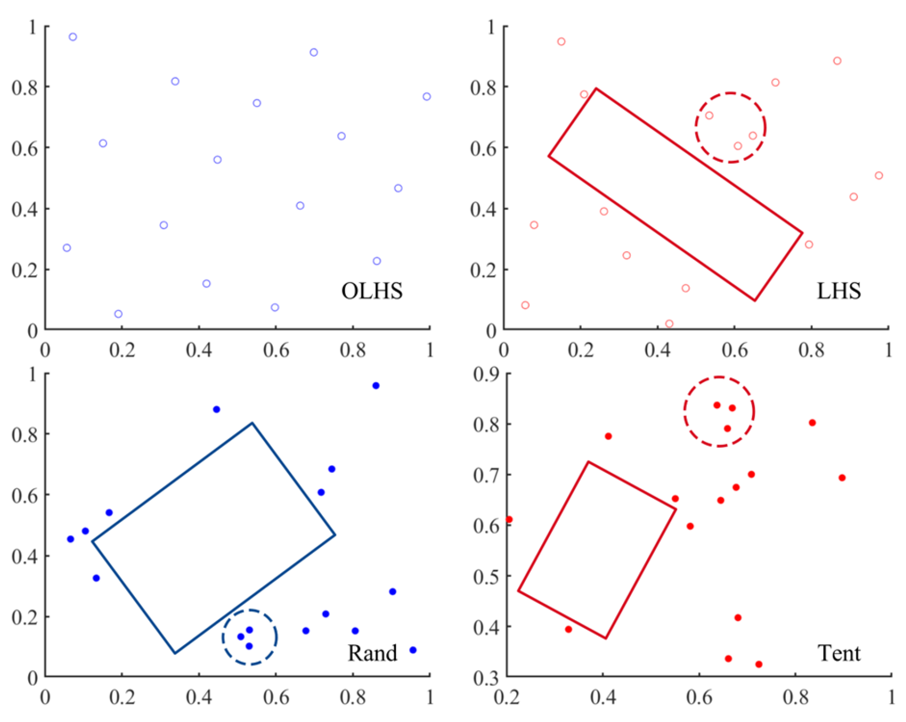
The random populations produced by the Rand function, Latin Hypercube Sampling (LHS), Tent Chaotic Mapping, and Optimal Latin Hypercube Sampling (OLHS) are compared in this paper.
Figure 2 demonstrates that, in contrast to the initial population generated by Optimal Latin Hypercubic Sampling (OLHS), populations generated by the Rand function, Latin Hypercubic Sampling (LHS), and Tent Chaotic Mapping exhibit uneven distribution patterns such as aggregation and over-dispersion.
Introducing Optimal Latin Hypercubic Sampling (OLHS) into the initialization function of the algorithm, a new initialization equation is obtained as follows:
where OLHS is a collection of random vectors produced by Optimal Latin Hypercube Sampling,
is the upper boundaries of the search space,
is the lower boundaries of the search space,
is the number of tuna populations.
2.2. Improved Spiral Foraging Strategy
To enhance the global exploration capability of the TSO algorithm during the initial phase, prevent falling into local optima, and enable the algorithm to converge rapidly in the later search stages, we propose introducing nonlinear dynamic weights to improve the original spiral foraging strategy. As the weight of the random term increases, the tuna swarm can traverse the search space more effectively, thereby enhancing exploration. Similarly, increasing the weight of the optimal term strengthens exploitation performance. The equation for the improved spiral foraging strategy is as follows:
where
is the
-th individual of the
-th iteration,
is randomized spiral foraging,
is optimal spiral foraging,
and
are nonlinear dynamic weighting coefficients,
denotes the initial value of
,
denotes the final value of
,
denotes the initial value of
,
denotes the final value of
,
and
are the current iteration number and the maximum iteration number, respectively, and
,
and
are control parameters that control the rate of change in the weights, and different problems can try to select different combinations of
and
to obtain a better solution. The weight control parameter
used in this paper is
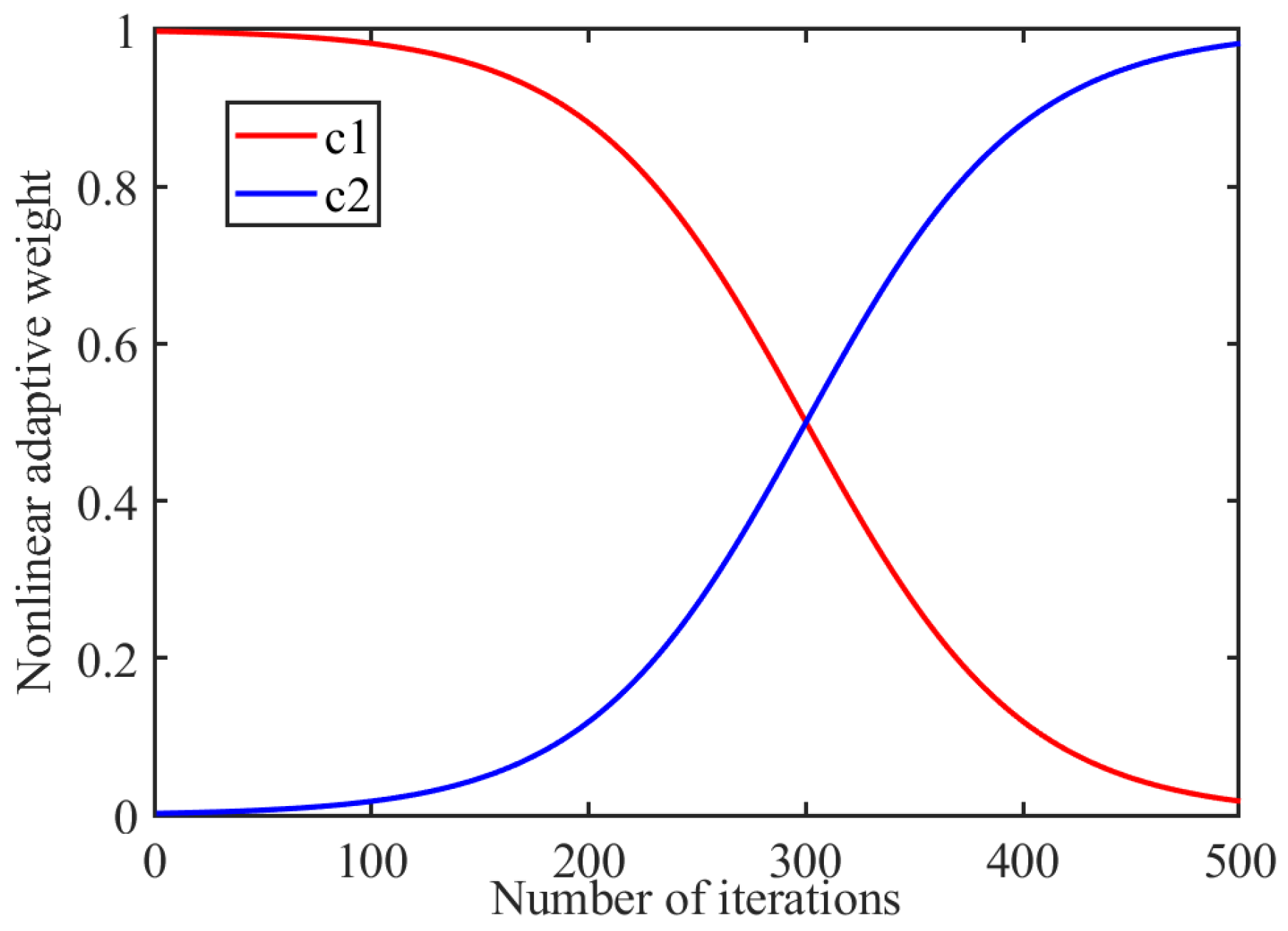
. The variation curve of nonlinear dynamic weights with the number of iterations is shown in
Figure 3.
The schematic illustrates how the random term serves as the dominant component in the early stages of the iteration to enhance the tuna swarm’s exploration capability. The optimal term becomes the dominant factor in the later stages of the iteration, improving the algorithm’s convergence performance.
2.3. Fast Non-Dominated Sorting Mechanism
Domination in optimization problems means that a particular solution is non-inferior to on the objective function in N dimensions and superior to in at least one dimension. Therefore, the relationship between the two can be called: dominates , denoted as (maximization problem). If there is no that is better than , then mark as a non-dominant individual (i.e., none is better than under the N-dimensional objective function).
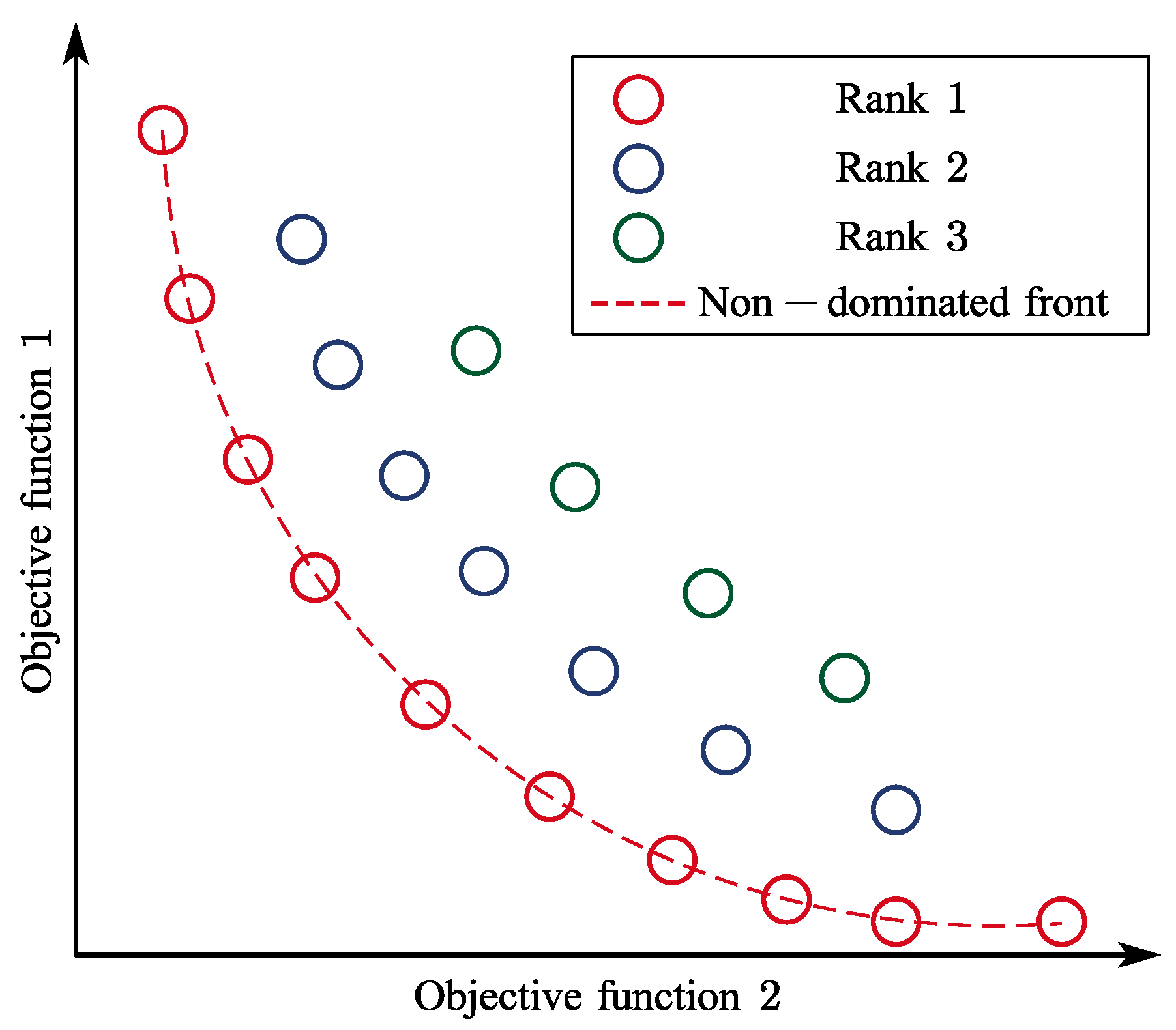
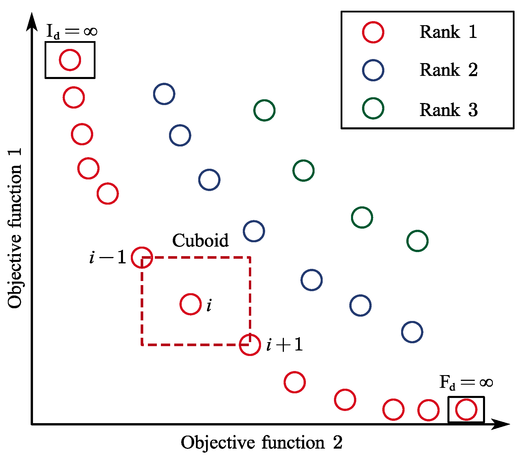
Non-dominated sorting is based on the dominance level to rank the Pareto-optimal solution and is assigned a rank based on its ability. A solution is referred to as Rank 1 when it is not dominated by other solutions, a solution dominated by only one solution is referred to as Rank 2, and a solution dominated by only two solutions is referred to as Rank 3, and so on.
As shown in
Figure 4, Rank 1 represents the first Pareto front, and Rank 2 represents the second Pareto front, where any solution in the first front dominates all solutions in the second front. This process classifies solution sets with identical objective function values into distinct Pareto fronts. Non-dominated sorting typically requires
computational complexity (where
denotes the number of objective functions and
the population size), with the computational cost scaling proportionally to both parameters.
Fast non-dominated sorting [
19] overcomes the shortcomings of excessive search iterations in conventional non-dominated sorting and reduces the computational complexity of the process, thereby decreasing the optimization algorithm’s complexity to
.
2.4. Crowding Distance and Crowding Comparison Operators
Lower crowding distances correspond to higher solution density and enhanced exploratory coverage, which mitigates premature convergence to local optima. Conversely, solutions with lower density indicate underutilized regions in the search space, suggesting continued exploration potential. To preserve solution diversity, individuals exhibiting larger crowding distances are prioritized during the subsequent selection phase.
Crowding distance is a measure of how densely packed the solutions are around each solution. As shown in
Figure 5, this value represents the perimeter of the rectangle formed by the nearest solutions as vertices. The diversity of the population is maintained by the crowding distance [
19].
Specific calculation steps:
① Initialize the crowding distance for each point: ;
② Non-dominated sorting of the population such that the 2-individual crowding distance at the boundary is infinity, i.e.,: ;
③ Crowding distance was calculated for the remaining
individuals:
where
denotes the crowding distance at point
,
denotes the
-th objective function value at point
, and
denotes the
-th objective function value at point
.
Crowding Comparison Operator: the premise of the comparison operator is that after the computation of the fast non-dominated sorting and the crowding distance, each individual in the population has two attributes: the non-dominated rank obtained from the non-dominated sorting and the crowding distance .
Based on these two properties, we can then define the congestion comparison operator: compare individual with individual . Individual wins if either of the following conditions holds.
① ; individual is in a better non-dominant rank than individual . The selected individual belongs to the better non-dominant rank.
② ; individual and individual have the same rank, but individual has a greater crowding distance. That is, the individual in the less crowded region is selected.
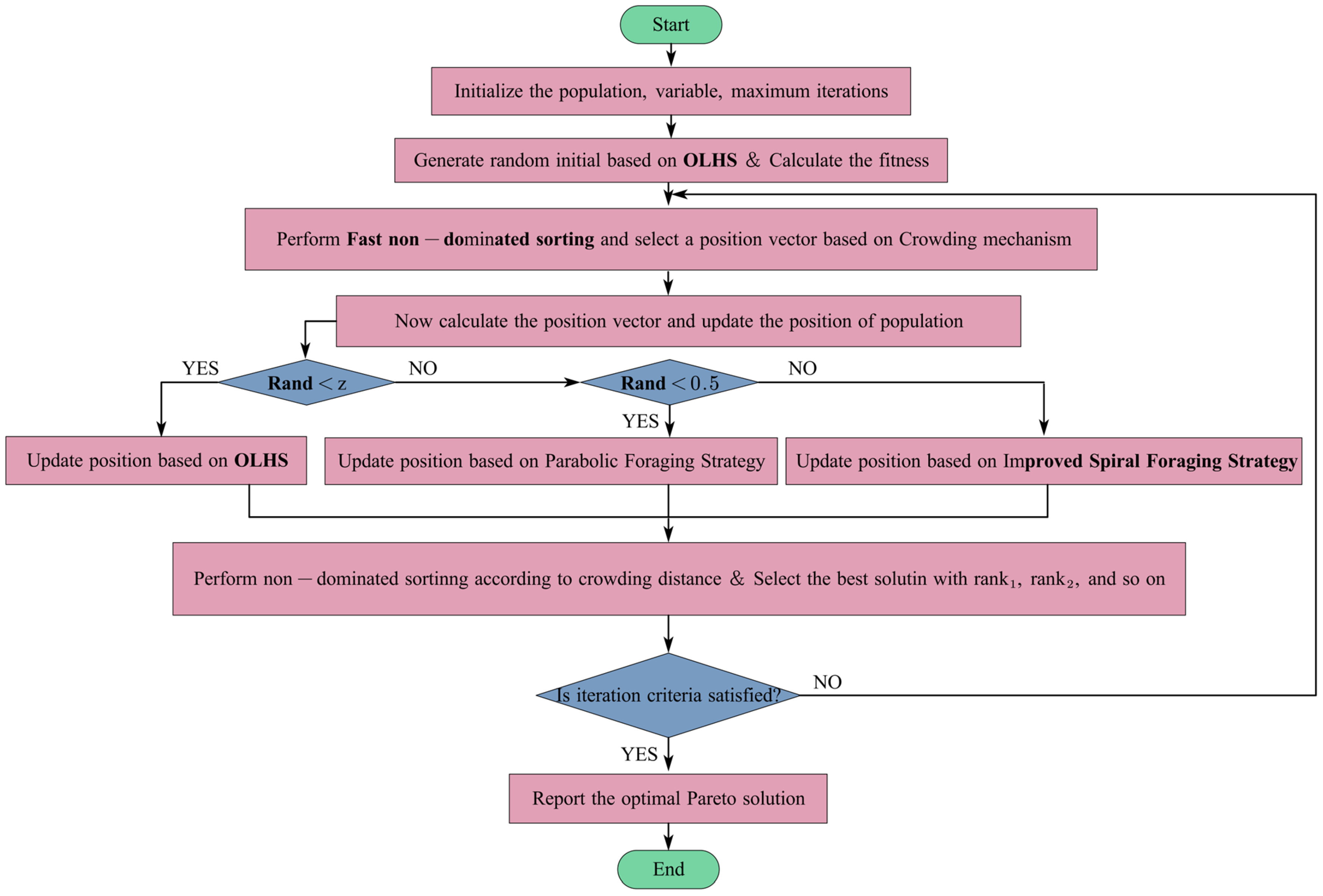
In summary, this paper proposes the following improvements to the TSO algorithm as shown in
Figure 6: Optimized Latin Hypercubic Sampling (OLHS) replaces the random function for population initialization, enhancing population distribution uniformity; a dynamic weighting coefficient improves the spiral foraging strategy, further balancing the “exploration” and “exploitation” trade-off while enhancing algorithmic robustness; and incorporating the fast non-dominated sorting mechanism with the crowding distance mechanism lowers computational complexity and yields a multi-objective variant of the algorithm.
2.5. Basic Work of the FNS-TSO Algorithm
The operational framework of the FNS-TSO algorithm is structured into four phases: Phase 1: The tuna population is initialized, and the fitness of the tuna swarm positions is calculated based on the objective function. Phase 2: The positions of the tuna swarms are updated through spiral or parabolic motion patterns. With equal probability (50%), the swarm follows either a spiral or parabolic path during optimization, thereby determining the next candidate positions. Phase 3: The FNS-TSO algorithm maintains the best Pareto solutions in an archive and allows dynamic adjustment of solutions during iterations. If the archive reaches capacity (exceeding a user-defined threshold), non-dominated solutions with larger crowding distances are selectively retained based on the crowding distance mechanism. Phase 4: Iteration termination: The search systematically terminates in uncertain search spaces when the maximum iteration threshold enforces convergence to the optimum. The FNS-TSO workflow is illustrated in
Figure 7.
4. Application of FNS-TSO in Underwater Manipulator Trajectory Optimization Problem
Underwater manipulators require smooth and stable operation to perform tasks such as grasping and exploration. When meeting impact constraints, it is essential to optimize the operational duration and energy consumption of underwater manipulators to improve work efficiency and reduce energy costs. Therefore, this paper establishes a trajectory model using quintic spline interpolation with three optimization objectives: total time, total energy consumption, and total impact for underwater manipulators. The FNS-TSO algorithm is then applied to perform trajectory optimization and obtain the Pareto optimal solution set.
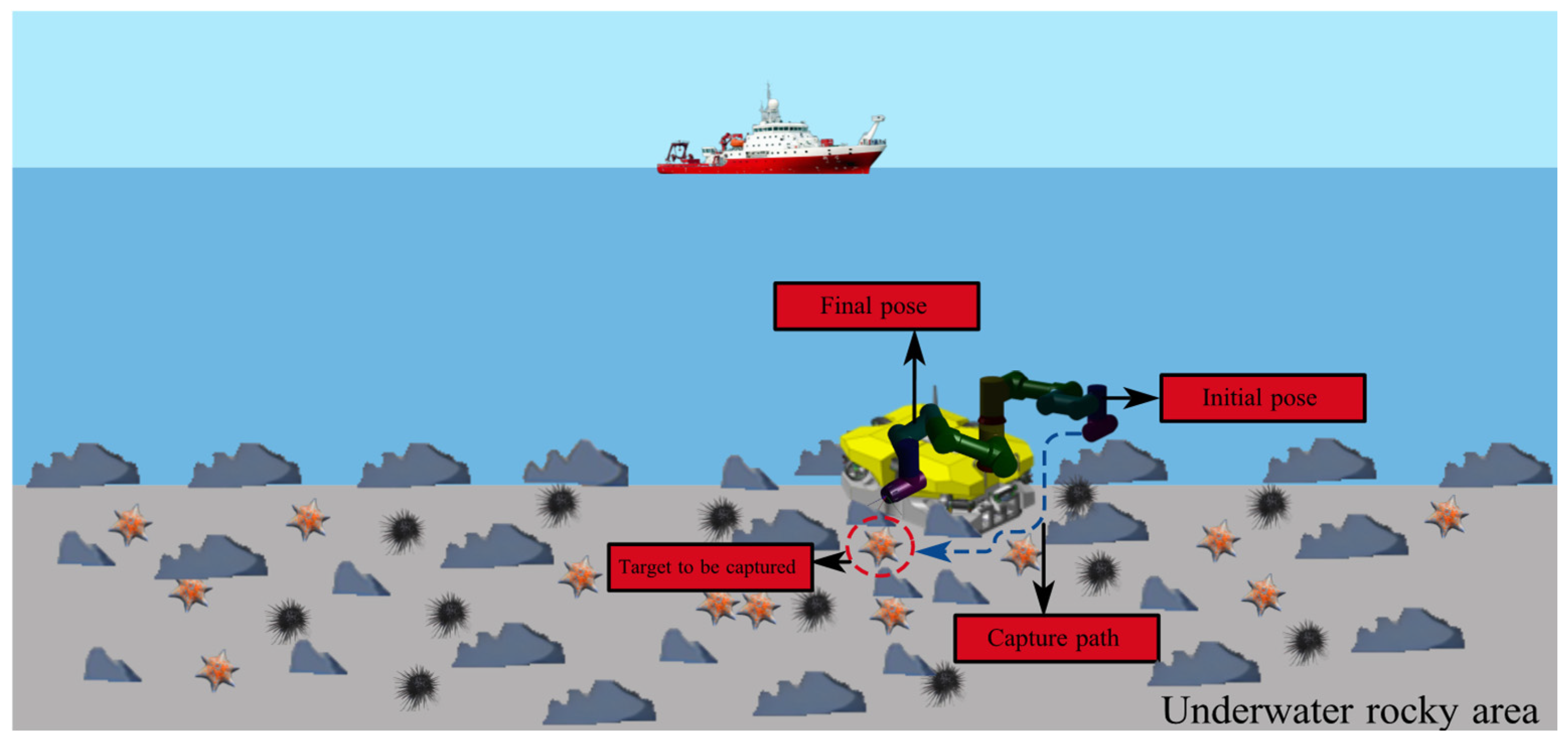
Our underwater manipulator is primarily employed for tasks such as underwater mineral collection and marine biological sample capture. As shown in
Figure 29, the underwater manipulator needs to complete point-to-point movement from the end of the arm to the object being grabbed during the task. Multiple path points can be selected between the starting and ending points, resulting in numerous potential paths traversing these points. It is necessary to choose the optimal path that achieves the time-energy-impact optimization. The optimal time aims to improve work efficiency and enable the acquisition of more mineral resources within a limited timeframe; the electric-driven manipulator can only carry a limited battery capacity during operation, and thus the optimal energy consumption addresses the limited energy capacity and the optimal impact ensures smoother operation.
4.1. Derivation of Quintic Spline Interpolation
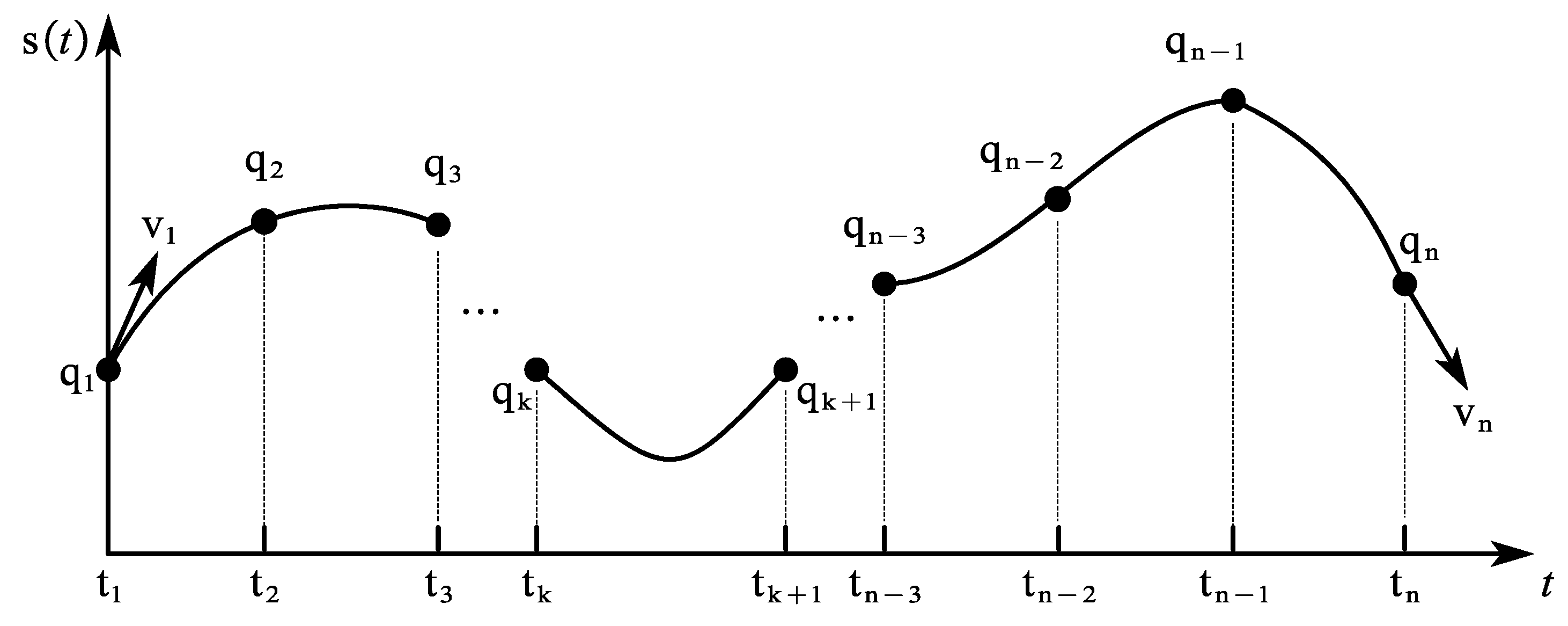
When given n points, instead of using a single quintic interpolating polynomial, we can employ n − 1 quintic polynomials, each defining a trajectory segment. The resulting composite function s(t) is called a fifth-order spline curve. Quintic spline interpolation ensures both smooth and continuous transitions of velocity and acceleration at all interpolation points while also guaranteeing zero initial and final velocities and accelerations in the planned trajectory. This significantly mitigates the start–stop shock in underwater manipulators.
Define the functional form of a quintic spline curve as:
This trajectory consists of
n − 1 quintic polynomials and each polynomial requires the computation of six parameters, resulting in a total of 6
n − 6 coefficients to be determined. As shown in
Figure 30, the initial velocity is
, the termination velocity is
, and under natural conditions, the acceleration
and
at the initial and final moments are both 0. To ensure the smoothness of position, velocity, and acceleration and reduce the impact during motion, quintic spline interpolation needs to satisfy the continuity of
,
,
,
,
.
where
.
From the interpolation condition:
And the spline curve is continuous at each segment transition, i.e:
Through deduction, the interpolation formula for the quintic spline is written in matrix form as:
4.2. Optimal Trajectory Planning Based on FNS-TSO
The decision variable for trajectory multi-objective optimization is the time length of each interpolation interval, denoted as , where , , denotes the time series of the trajectory points, and the time of the first point is , usually taken as . The defined optimization objective function and the constraints are shown below.
Objective function:
where
is the time optimum,
denotes the number of interpolation intervals,
is the energy objective function,
denotes the acceleration variable for each interval,
is the objective function of the shock, and
denotes the additive acceleration variable for each interpolation interval.
Constraints:
where
and
, respectively, denote the speed at which the
-th joint operates and the maximum joint speed allowed,
and
respectively denote the acceleration at which the
-th joint operates and the maximum joint acceleration allowed, and
and
denote the accelerated acceleration at which the
-th joint operates and the maximum joint accelerated acceleration allowed, respectively.
Assuming that the underwater manipulator needs to move along a curve L in Cartesian space to accomplish the task of handling minerals on the seafloor, the position parameters
of the passing points are as shown in
Table 4.
Through the kinematic inverse solution, the angular interpolation points of the six joints were obtained, which are shown in
Table 5.
The value range of the decision variables is
, and the velocity and acceleration at the start and end points of the underwater manipulator are set to 0. The constraints are:
The times for each interpolation interval for the underwater manipulator selected before optimization are shown in
Table 6.
Based on the timings listed in the table, quintic spline interpolation is performed, and the motion parameters’ variation of each joint in the underwater manipulator is simulated using MATLAB(R2023b), as shown in
Figure 31.
The simulation results show that the joint trajectories are smooth and continuous, with velocities and accelerations at the start and end being zero. However, during the initial movement phase, joints 2 and 3 exhibit excessive impact forces, while joints 2 and 4 demonstrate similar issues in the final phase, causing the joint jerk to exceed the specified threshold. Furthermore, parameters such as time, energy, and impact fail to reach optimal values.
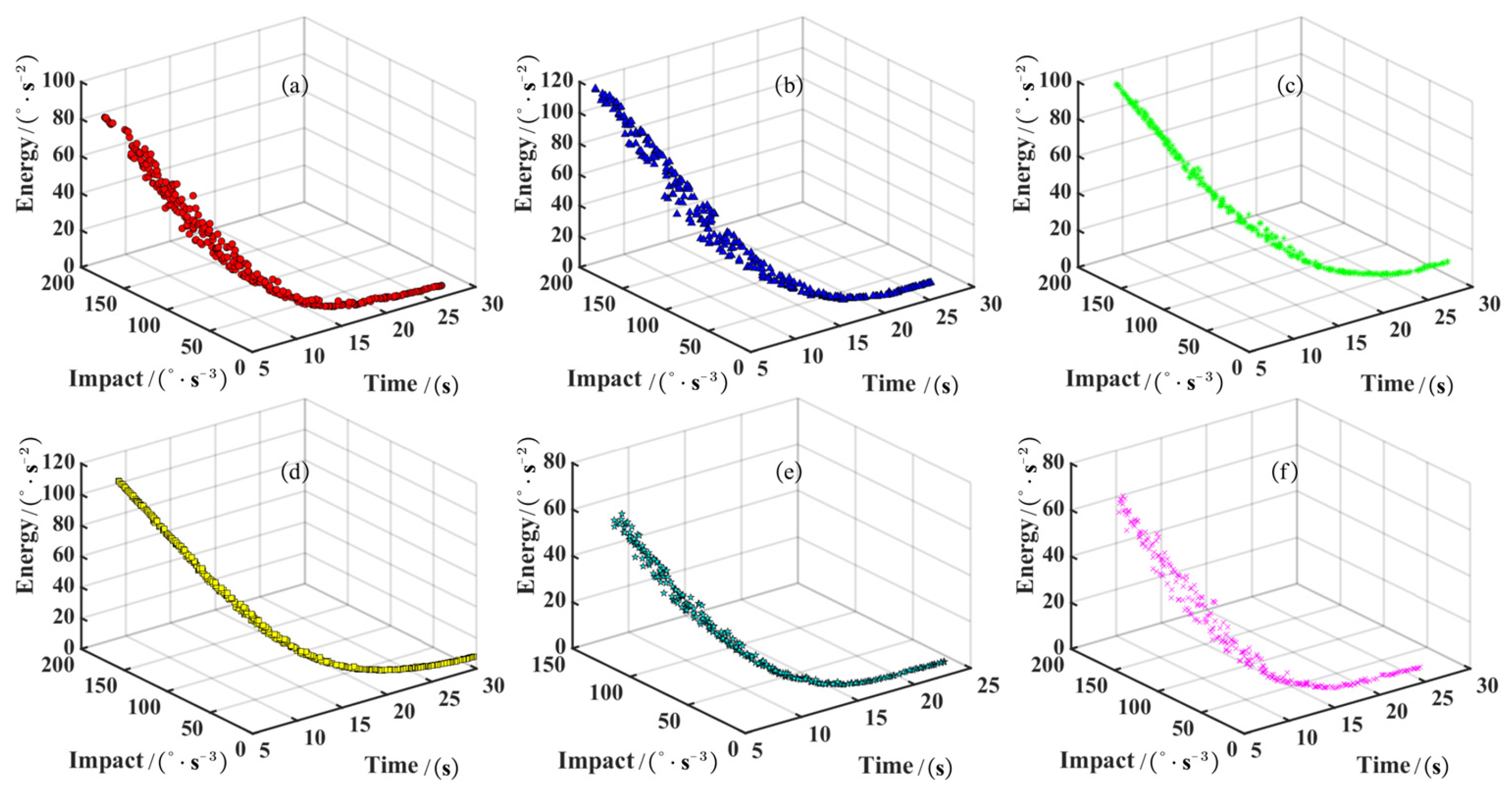
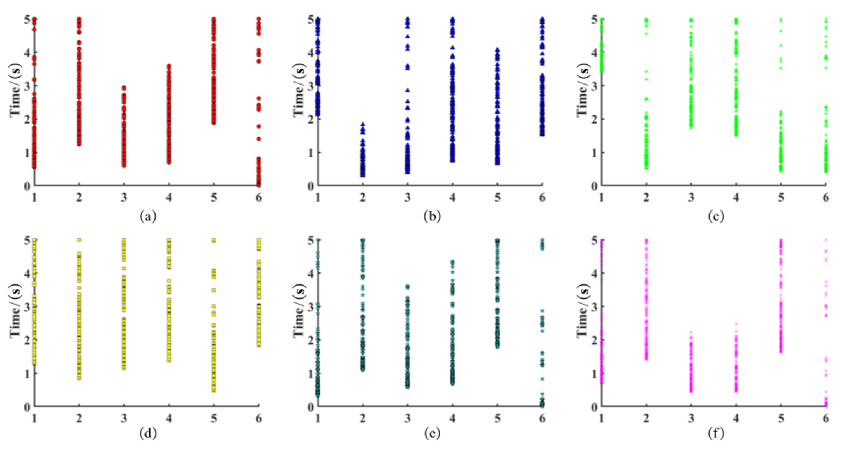
The FNS-TSO algorithm was applied to conduct multi-objective optimization for each joint of the underwater manipulator independently, with a population size and maximum iteration count of 300 each. This process generated the Pareto front and population distribution for each joint, as illustrated in
Figure 32 (Pareto fronts) and
Figure 33 (population distributions), respectively.
From the Pareto frontiers, analysis reveals an inverse relationship between time and energy consumption/impact: extended durations correspond to lower energy consumption and reduced impact, while shorter durations exhibit higher energy consumption and amplified impact. Therefore, engineering applications require selection based on actual operational constraints. This study prioritizes energy efficiency and impact mitigation, selecting a balanced time duration through multi-criteria analysis (see
Table 7).
To ensure synchronized joint movements in underwater manipulators, the maximum joint movement time is selected for each segment of the interval, as detailed in
Table 8.
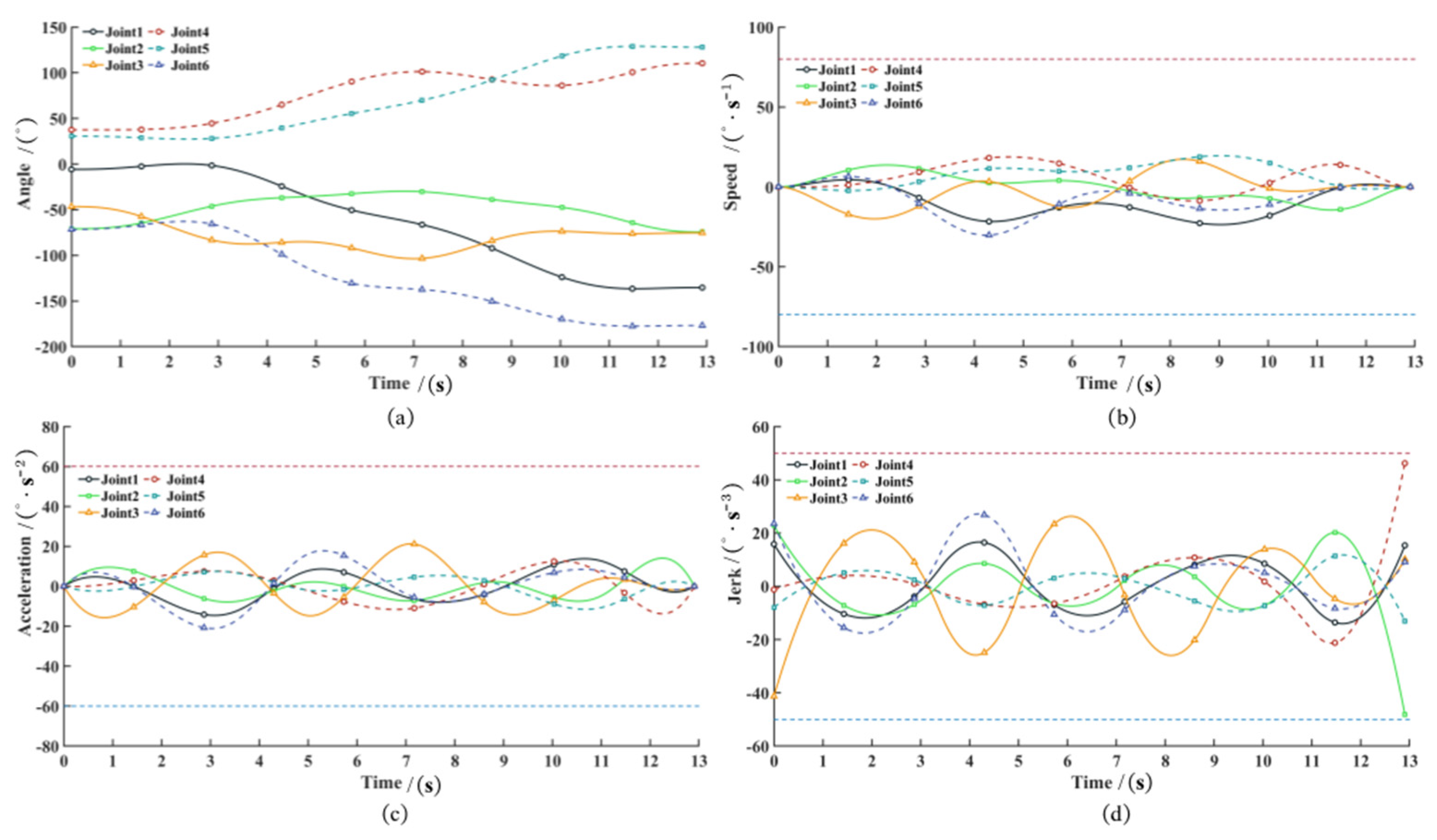
The variations in angle, angular velocity, angular acceleration, and jerk of the optimal quintic spline trajectories for each joint are shown in
Figure 34.
The simulation results demonstrate that the optimally planned trajectory is smooth, continuous, and free of abrupt changes. The manipulator’s end-effector passes precisely through all predefined path points, while joint speed, acceleration, and jerk remain within constraint limits throughout the operation. The quintic spline trajectory fully satisfies all technical requirements. Quantitative comparisons of the underwater manipulator’s total operation time, total joint energy consumption, and impact before and after optimization are presented in
Table 9.
The tabular data demonstrate that the manipulator’s total operation time decreases by 11.03%, with 19.02% reduction in energy consumption and 24.69% mitigation of total impact compared to pre-optimization benchmarks. The multi-objective optimized trajectory therefore ensures smooth underwater operation while enhancing efficiency and significantly reducing energy expenditure.
