Article

Fast Non-Dominated Sorting Tuna Swarm Optimization Algorithm (FNS-TSO): Time-Energy-Impact Multi-Objective Optimization of Underwater Manipulator Trajectories

1
Institute of Marine Science and Technology, Shandong University, Qingdao 266237, China
2
School of Mechanical Engineering, Shandong University, Jinan 250061, China
3
Key Laboratory of High Efficiency and Clean Mechanical Manufacture, Ministry of Education, Jinan 250061, China
*
Author to whom correspondence should be addressed.
J. Mar. Sci. Eng. 2025, 13(5), 916; https://doi.org/10.3390/jmse13050916
Submission received: 27 March 2025 / Revised: 1 May 2025 / Accepted: 3 May 2025 / Published: 6 May 2025
(This article belongs to the Section Ocean Engineering)

Abstract

:
To achieve time–energy–impact multi-objective optimization in the trajectory control of underwater manipulators, this paper proposes a Fast Non-Dominated Sorting Tuna Swarm Optimization algorithm (FNS-TSO). The algorithm integrates a fast non-dominated sorting mechanism into the Tuna Swarm Optimization algorithm, improves initialization through Optimal Latin Hypercubic Sampling (OLHS) to enhance population distribution uniformity, and incorporates a nonlinear dynamic weight to refine the spiral foraging strategy, thereby strengthening algorithmic robustness. To verify FNS-TSO’s effectiveness, we conducted comparative evaluations using standard test functions against three established algorithms: Multi-Objective Particle Swarm Optimization (MOPSO), Multi-Objective Jellyfish Search Optimization (MOJSO), and the Non-Dominated-Sorting Genetic Algorithm (NSGA-II). Results demonstrate superior overall performance, particularly regarding convergence speed and solution diversity, with solution set distributions showing enhanced uniformity. In practical implementation, we applied FNS-TSO to the multi-objective optimization of an underwater manipulator using quintic spline curves for trajectory planning. Simulation outcomes reveal respective reductions of 11.03% in total operation time, 19.02% in energy consumption, and 24.69% in mechanical impacts, with the optimized manipulator achieving stable point-to-point motion transitions.

1. Introduction

The optimization algorithm is a mathematical technique for determining the optimal solution to a problem given constraints or limitations. In contemporary research, a wide range of disciplines, including prediction, control, and mechanical systems, employ optimization methodologies. Current research on optimization algorithms focuses on achieving optimal solutions with minimal computational time and resources while balancing global and local search capabilities. Early-stage optimization algorithms require significant computational resources and labor and suffer from issues such as overreliance on initial solutions and local minima stagnation [1,2]. Furthermore, most real-world models requiring optimization exhibit complex constraints, high-dimensional decision variables, and pronounced nonlinear properties, posing challenges for effective algorithmic solutions [3,4]. Consequently, researchers have proposed metaheuristic algorithms to address the complexity and computational challenges of optimization processes.
Typically, metaheuristic algorithms fall into three categories [5]: evolution-based algorithms, physics-based algorithms, and population-based algorithms. Among these, evolution-based algorithms draw inspiration from natural evolution. The most prominent example is the Genetic Algorithm (GA), proposed by Holland in 1992, which implements Darwinian evolutionary theory [6]. Physics-based algorithms emulate physical laws; the classic example is the Simulated Annealing Algorithm (SA), proposed by Kirkpatrick et al. in 1983 [7]. SA models the metallurgical annealing process and probabilistically accepts suboptimal solutions to escape local optima. Currently, the most popular and rapidly evolving stochastic algorithms are population-based algorithms, which mimic collective behaviors in biological populations. Two classical examples are Particle Swarm Optimization (PSO) [8] (Kennedy et al., 1995) and Ant Colony Optimization (ACO) [9] (Dorigo et al., 2006). PSO simulates avian flocking behavior, while ACO emulates ant foraging strategies. Subsequent developments have produced algorithms such as the Krill Herd Algorithm (KH) [10], Gray Wolf Optimization (GWO) [11], the Whale Optimization Algorithm (WOA) [12], Tuna Swarm Optimization (TSO) [13], and Hippopotamus Optimization (HO) [14]. These algorithms are valued for their model independence, gradient-free operation, robust global search capability, versatility, and computational efficiency [15].
Most engineering problems require multi-objective rather than single-objective optimization. For example, an underwater manipulator operates as a multibody dynamic system that simultaneously requires optimization of joint kinematics, motion duration, energy consumption, and vibration suppression. In nonlinear multi-objective optimization, conflicting objectives often arise where some functions require maximization while others necessitate minimization. Unlike single-objective problems, the solution involves identifying Pareto-optimal solutions that represent the best achievable trade-offs between competing objectives. Consequently, developing robust multi-objective optimization algorithms constitutes the current research frontier in this field.
Currently, researchers primarily employ Pareto dominance and non-dominated sorting mechanisms to enhance single-objective optimization algorithms for multi-objective optimization. The most widely used algorithms include Multi-Objective Particle Swarm Optimization (MOPSO) [16,17], proposed by Coello et al., which integrates Pareto dominance into Particle Swarm Optimization (PSO) to handle multi-objective problems; the Non-Dominated Sorting Genetic Algorithm (NSGA) [18], developed by Deb and Srinivas using non-dominated sorting to upgrade single-objective algorithms; NSGA-II [19], an improved version by Deb et al. featuring a computationally efficient fast non-dominated sorting mechanism; other variant algorithms, such as Multi-Objective Gray Wolf Optimization (MOGWO) [20], the Non-Dominated Sorting Whale Optimization Algorithm (NSWOA) [21], the Multi-Objective Whale Optimization Algorithm (MOWOA) [22], Non-Dominated Sorting Gray Wolf Optimization (NSGWO) [23], the Multi-Objective Jellyfish Search Optimizer (MOJSO) [24], and Multi-Objective Tuna Swarm Optimization (MOTSO) [25]. However, existing multi-objective algorithms exhibit limitations in universal applicability. The No-Free-Lunch Theorem motivates researchers to develop novel metaheuristics or refine existing algorithms for domain-specific optimization challenges [26].
At present, numerous researchers have optimized manipulator trajectories using multi-objective optimization algorithms. Huang et al. [27] employed the Multi-Objective Particle Swarm Optimization (MOPSO) method to solve an objective function comprising motion time, dynamic perturbation, and acceleration, obtaining an efficient and safe motion trajectory for a space robot. Marcos et al. [28] combined the closed-loop pseudo-inverse method with a Multi-Objective Genetic Algorithm (MOGA) to minimize joint displacements and end-effector position errors. Zhou et al. [29] proposed a time-optimal trajectory planning method for manipulators based on an improved butterfly algorithm. Yang et al. [30] developed a time-optimal trajectory planning method using the Marine Predators Algorithm (MPA) to satisfy the high-efficiency and high-precision operational requirements of manipulators. Additionally, other scholars have utilized and enhanced NSGA-II for manipulator trajectory optimization [31,32,33,34]. Due to the more complex working environments and the need to maintain stable and efficient operations, underwater manipulators face more challenging trajectory control compared to their land-based counterparts. Consequently, optimization outcomes for time, energy, and impact must meet stricter criteria. It is therefore insufficient to address underwater manipulators’ operational requirements by optimizing solely time or individual objective functions. The Tuna Swarm Optimization (TSO) algorithm exhibits rapid convergence, high solution accuracy, and excellent flexibility and scalability. It has been successfully applied to diverse optimization problems, including wind turbine fault classification [35], autonomous underwater vehicle path planning [36], Unmanned Aerial Vehicle (UAV) path planning [37], and other domains with demonstrated efficacy.
Therefore, in this paper, the Fast Non-Dominated Sorting Tuna Swarm Optimization algorithm (FNS-TSO) is proposed by improving the TSO algorithm and is used to optimize the trajectory of an underwater manipulator. The main novel contributions of this study are as follows: 1. integrating the fast non-dominated sorting mechanism into the TSO algorithm; 2. improving the initialization of FNS-TSO by Optimal Latin Hypercube Sampling; 3. designing a nonlinear dynamic weight to improve the convergence and robustness of the FNS-TSO algorithm.
This paper is structured as follows: Section 2 introduces the proposed FNS-TSO algorithm. 
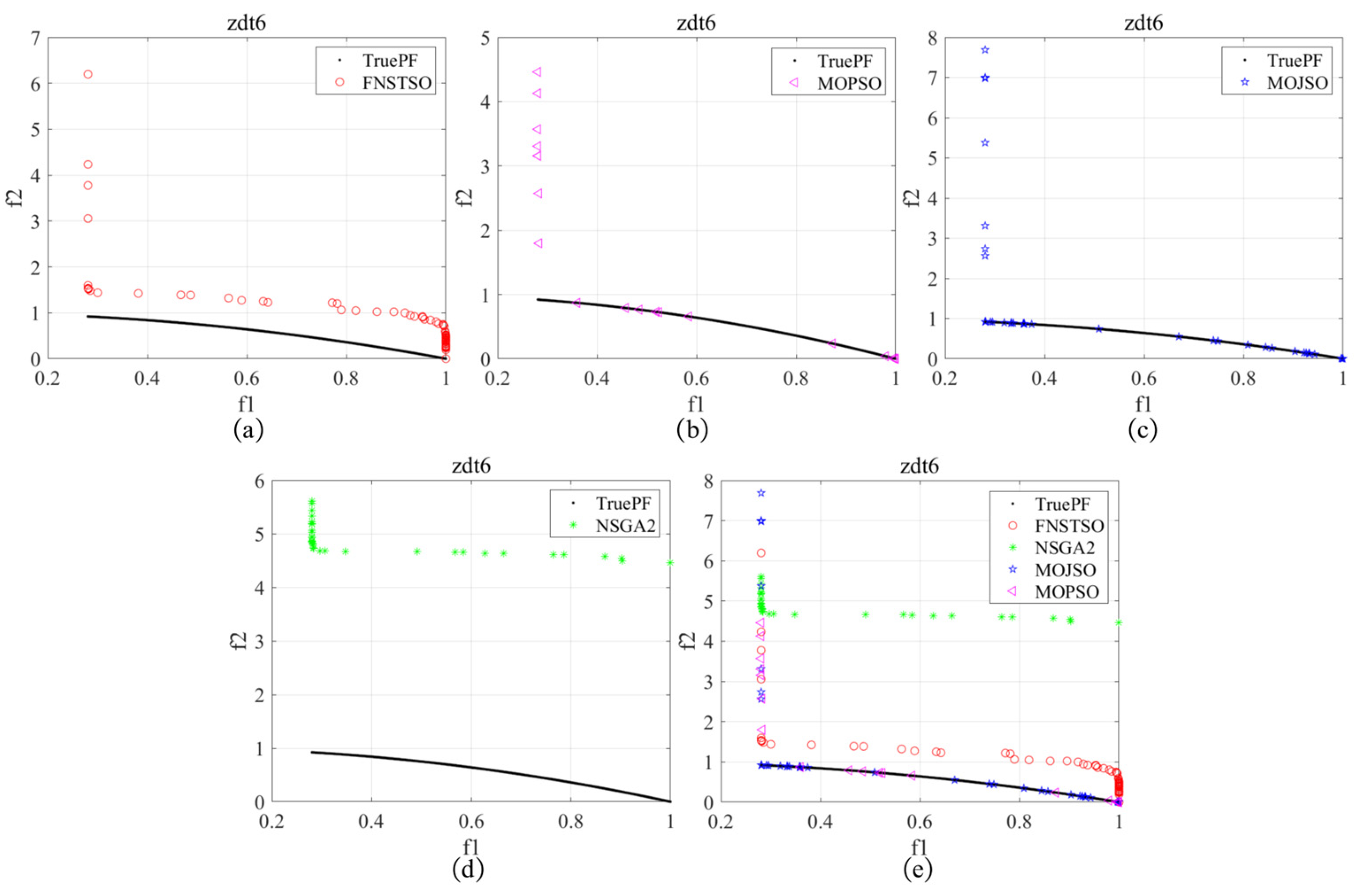
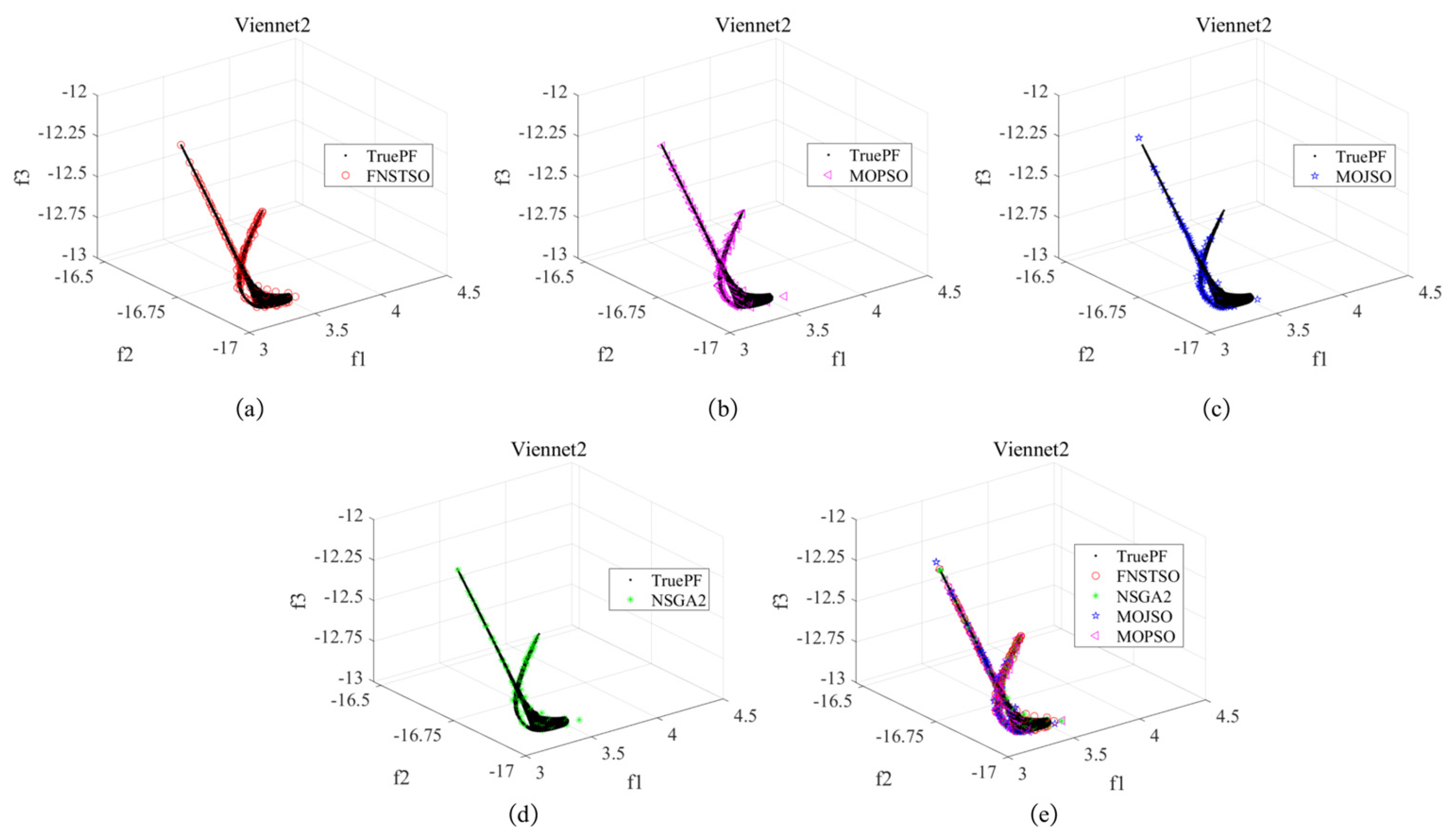
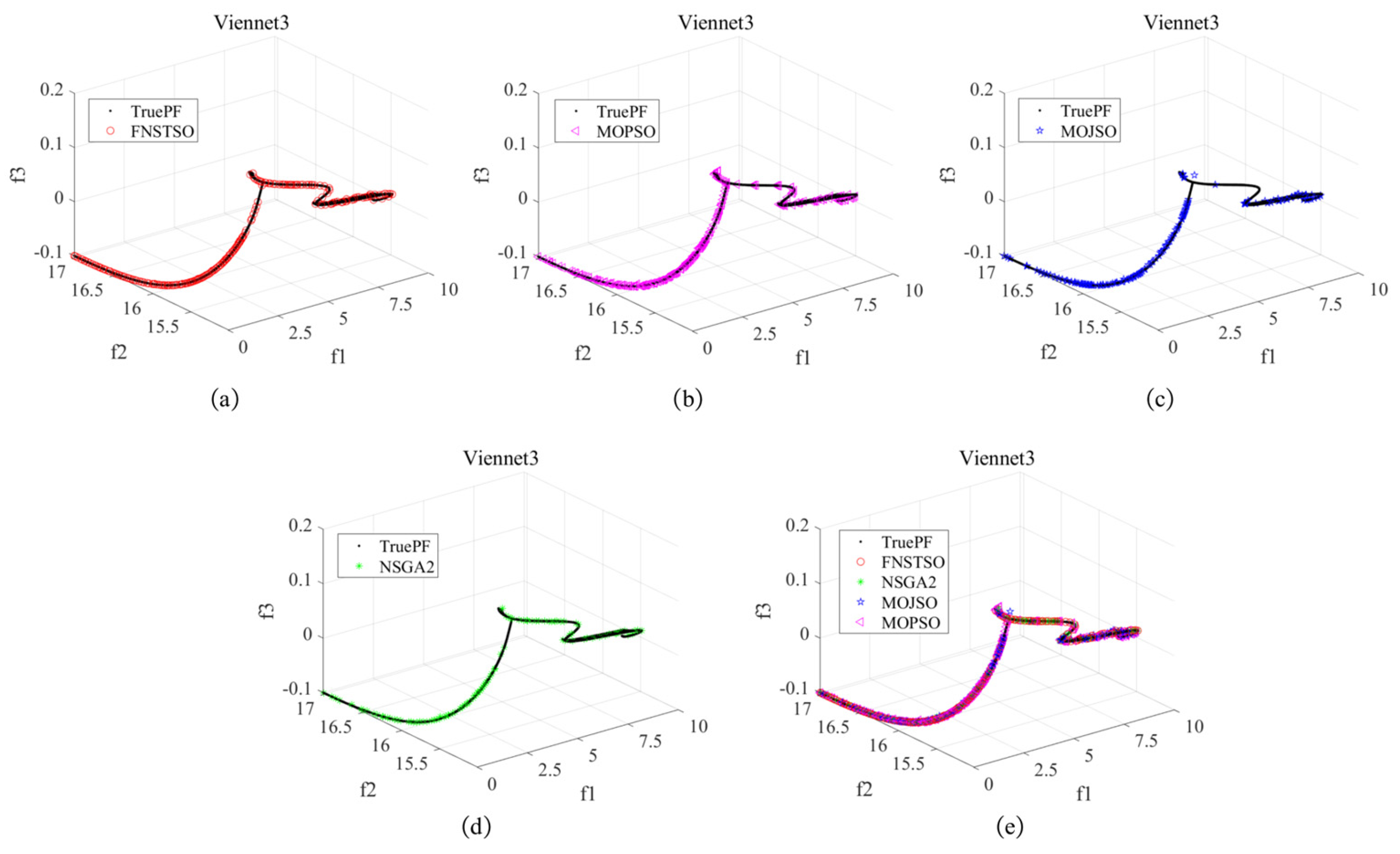
Section 3 presents a comparative analysis of the standard test function optimization results. Section 4 demonstrates the algorithm’s application in underwater manipulator trajectory optimization. Section 5 summarizes the key findings and provides actionable recommendations for future research.

2. Fast Non-Dominated Sorting Tuna Swarm Optimization (FNS-TSO)

The Tuna Swarm Optimization (TSO) algorithm is a new population-based metaheuristic optimization algorithm proposed by Xie et al. in 2021 [13], based on modeling two foraging behaviors (spiral foraging and parabolic foraging) of tuna swarms. This section focuses on the improvements made to the TSO algorithm and does not provide a detailed description of the underlying algorithm.

2.1. Optimal Latin Hypercube Sampling Initialization Strategy

Latin Hypercubic Sampling (LHS) is a stratified sampling technique for approximate random sampling from multivariate parameter distributions, first proposed by McKay et al. [38] and widely applied in multidisciplinary fields.
Following Mckay et al. in 1979 [38], let A = ( a i k ) be a Latin hypercube of n runs for q factors that is a n × q matrix where each column is obtained as a uniform permutation on Z n ( a 1 k , a 2 k , , a n k ) and these columns are obtained independently. A n × q Latin hypercube design D based on A is generated through [38]:
X i k = ( a i k u i k ) / n , ( i = 1 , 2 , , n , k = 1 , 2 , , q )
Specific explanations are provided in Appendix A.1.
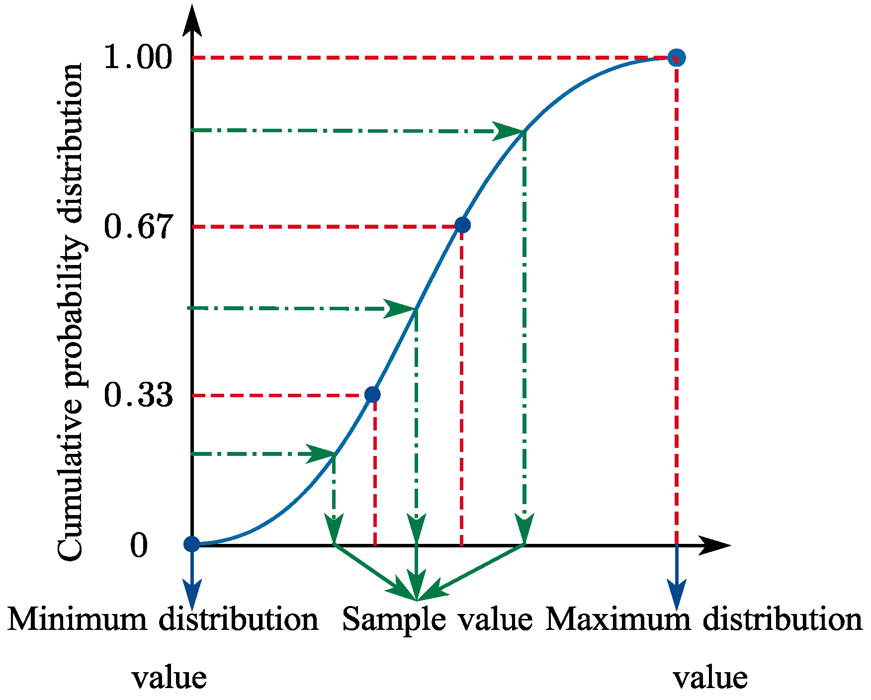
Stratifying the input probability distribution is fundamental to Latin Hypercube Sampling. On the cumulative probability scale (0 to 1.0), this method divides the cumulative distribution curve into equal intervals. A random sample is then selected from each stratum (or interval) of the input distribution.
The cumulative probability distribution function curve is separated into three intervals, as illustrated in Figure 1. One sample is drawn from each interval, and the interval is excluded from subsequent sampling once sampled. In practical applications, this approach proves efficient because the samples can more accurately reflect input probability distributions, avoiding the “clustering” phenomenon that may occur with small sample sizes.
The optimal design used in this paper is called a maximin distance design if it maximizes the minimum inter-site distance [39]:
min 1 i , j n , i j d ( x i , x j )
d ( x i , x j ) = d i j = k = 1 m x i k x j k t 1 / t , t = 1   o r   2
Specific explanations are provided in Appendix A.1.
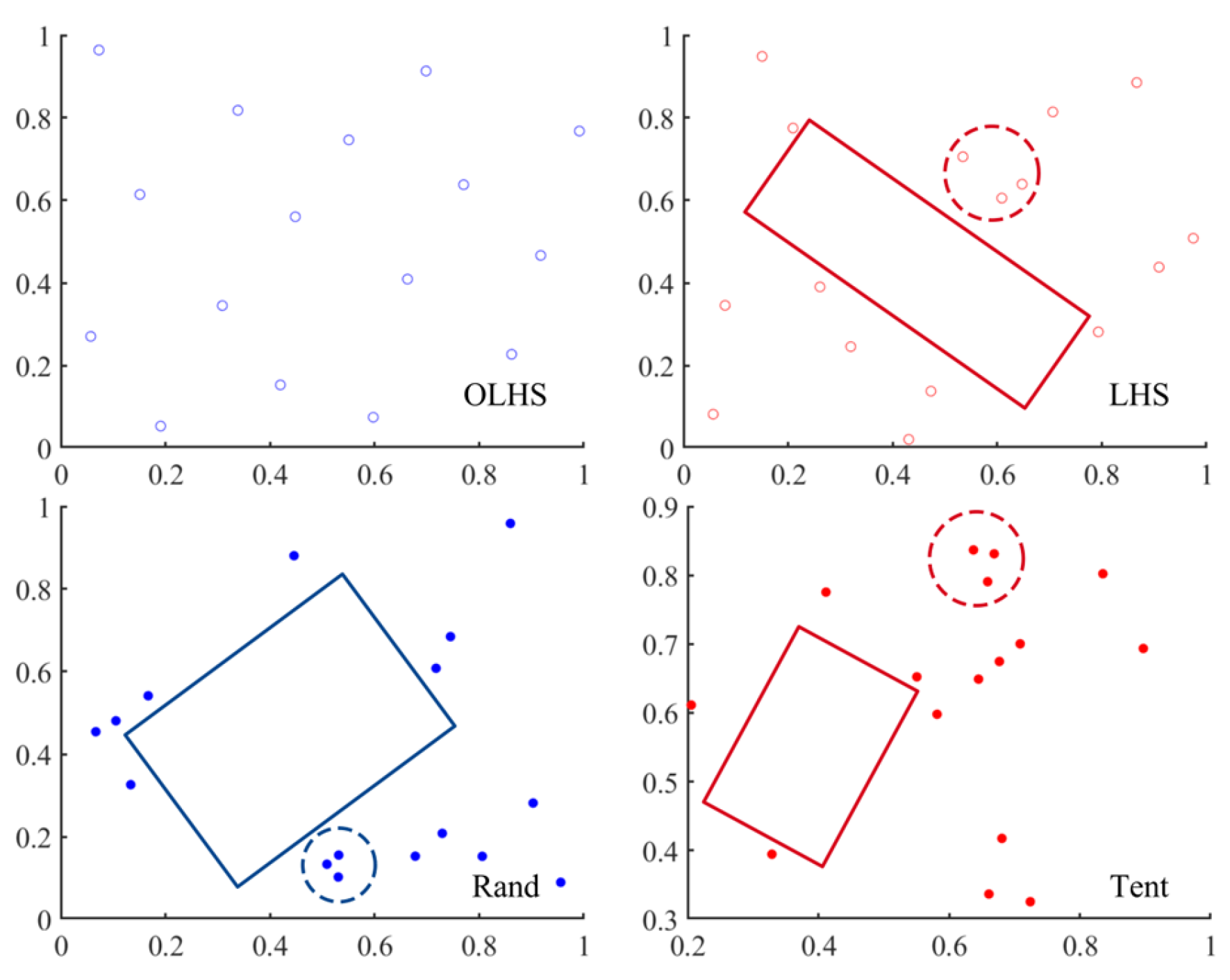
The random populations produced by the Rand function, Latin Hypercube Sampling (LHS), Tent Chaotic Mapping, and Optimal Latin Hypercube Sampling (OLHS) are compared in this paper.
Figure 2 demonstrates that, in contrast to the initial population generated by Optimal Latin Hypercubic Sampling (OLHS), populations generated by the Rand function, Latin Hypercubic Sampling (LHS), and Tent Chaotic Mapping exhibit uneven distribution patterns such as aggregation and over-dispersion.
Introducing Optimal Latin Hypercubic Sampling (OLHS) into the initialization function of the algorithm, a new initialization equation is obtained as follows:
X i int = OLHS · ( u b l b ) + l b , i = 1 , 2 , , N
where OLHS is a collection of random vectors produced by Optimal Latin Hypercube Sampling, u b is the upper boundaries of the search space, l b is the lower boundaries of the search space, N is the number of tuna populations.

2.2. Improved Spiral Foraging Strategy

To enhance the global exploration capability of the TSO algorithm during the initial phase, prevent falling into local optima, and enable the algorithm to converge rapidly in the later search stages, we propose introducing nonlinear dynamic weights to improve the original spiral foraging strategy. As the weight of the random term increases, the tuna swarm can traverse the search space more effectively, thereby enhancing exploration. Similarly, increasing the weight of the optimal term strengthens exploitation performance. The equation for the improved spiral foraging strategy is as follows:
X i t + 1 = c 1 X i t + 1 r a n d + c 2 X i t + 1 b e s t
c 1   =   c 1 i n i ( c 1 i n i c 1 f i n ) sigmoid t × Δ s t max s max c 2 = c 2 i n i ( c 2 i n i c 2 f i n ) sigmoid t × Δ s t max s max
where X i t + 1 is the i -th individual of the t + 1 -th iteration, X i t + 1 r a n d is randomized spiral foraging, X i t + 1 b e s t is optimal spiral foraging, c 1 and c 2 are nonlinear dynamic weighting coefficients, c 1 i n i denotes the initial value of c 1 , c 1 f i n denotes the final value of c 1 , c 2 i n i denotes the initial value of c 2 , c 2 f i n denotes the final value of c 2 , t and t max are the current iteration number and the maximum iteration number, respectively, and Δ s = s max s min , s max and s min are control parameters that control the rate of change in the weights, and different problems can try to select different combinations of s max and s min to obtain a better solution. The weight control parameter ( s max , s min ) used in this paper is ( 6 , 4 ) 
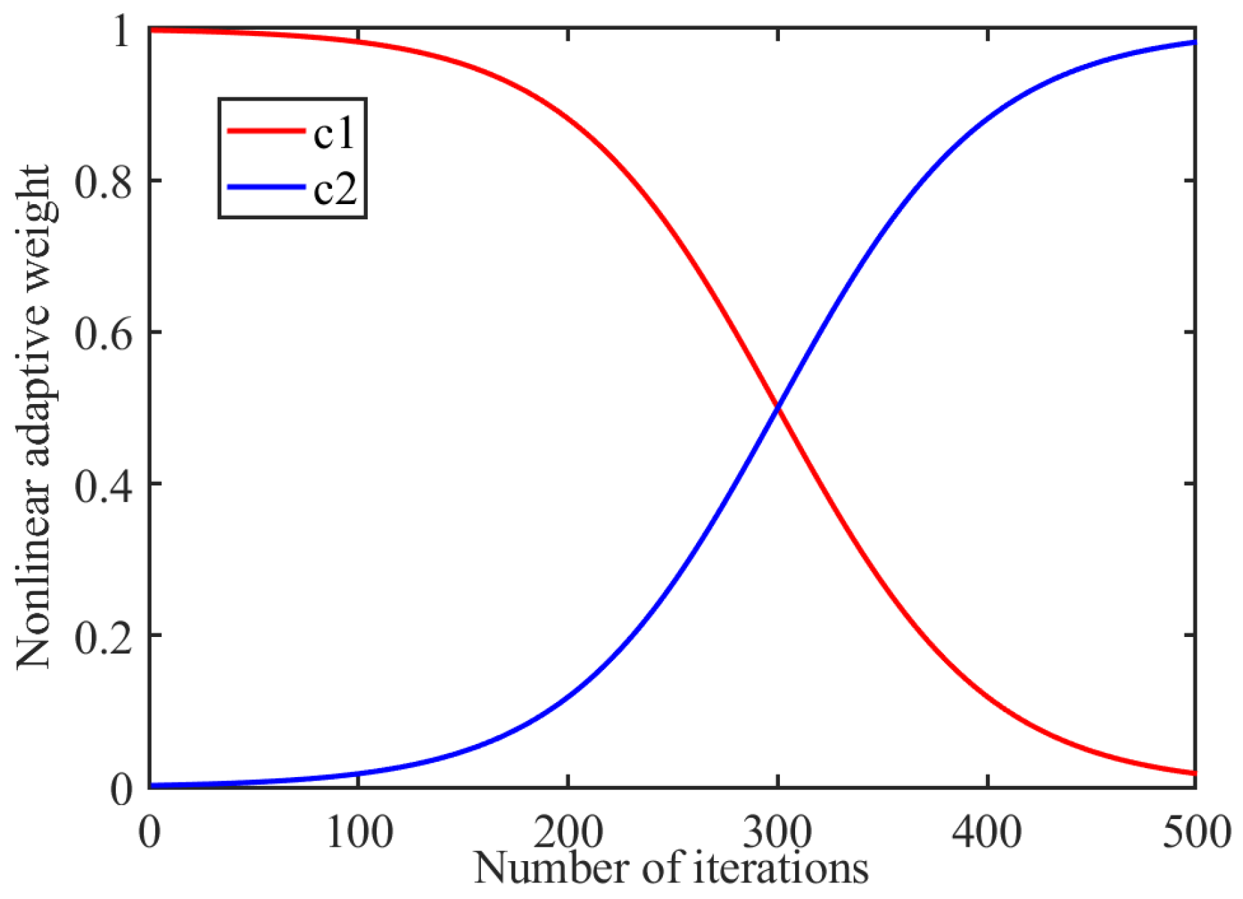
. The variation curve of nonlinear dynamic weights with the number of iterations is shown in Figure 3.
The schematic illustrates how the random term serves as the dominant component in the early stages of the iteration to enhance the tuna swarm’s exploration capability. The optimal term becomes the dominant factor in the later stages of the iteration, improving the algorithm’s convergence performance.

2.3. Fast Non-Dominated Sorting Mechanism

Domination in optimization problems means that a particular solution x i is non-inferior to x j on the objective function in N dimensions and superior to x j in at least one dimension. Therefore, the relationship between the two can be called: x i dominates x j , denoted as x i x j (maximization problem). If there is no x j that is better than x i , then mark x i as a non-dominant individual (i.e., none is better than x i under the N-dimensional objective function).
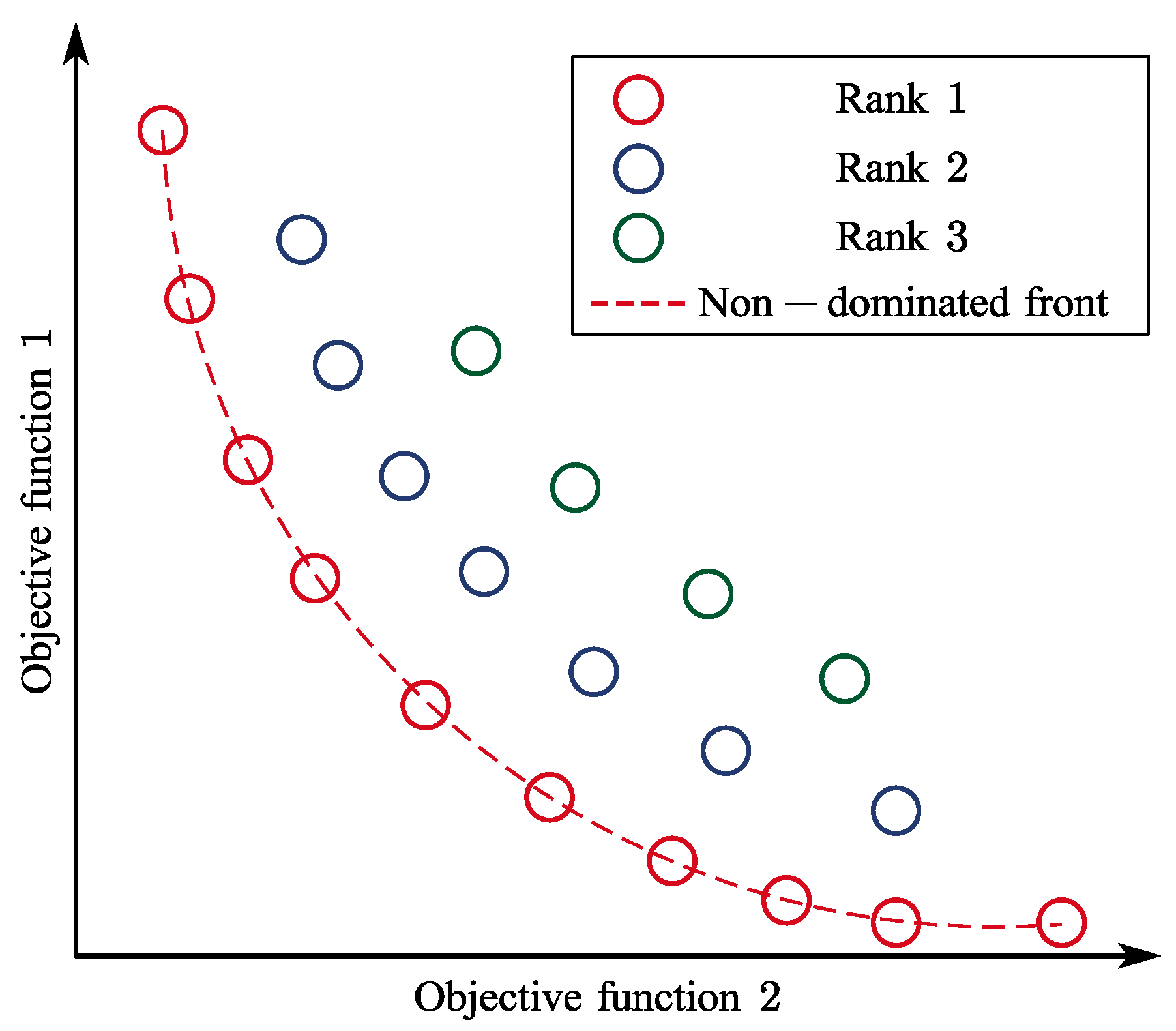
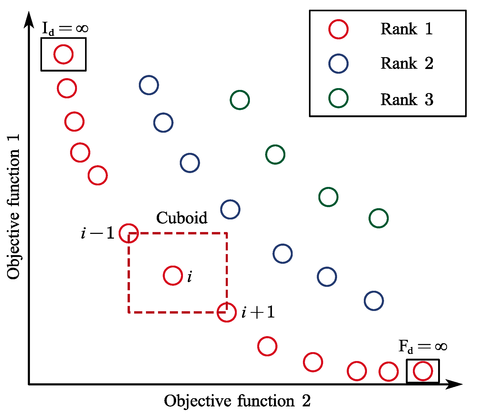
Non-dominated sorting is based on the dominance level to rank the Pareto-optimal solution and is assigned a rank based on its ability. A solution is referred to as Rank 1 when it is not dominated by other solutions, a solution dominated by only one solution is referred to as Rank 2, and a solution dominated by only two solutions is referred to as Rank 3, and so on.
As shown in Figure 4, Rank 1 represents the first Pareto front, and Rank 2 represents the second Pareto front, where any solution in the first front dominates all solutions in the second front. This process classifies solution sets with identical objective function values into distinct Pareto fronts. Non-dominated sorting typically requires o ( m N 3 ) computational complexity (where m denotes the number of objective functions and N the population size), with the computational cost scaling proportionally to both parameters.
Fast non-dominated sorting [19] overcomes the shortcomings of excessive search iterations in conventional non-dominated sorting and reduces the computational complexity of the process, thereby decreasing the optimization algorithm’s complexity to o ( m N 2 ) .

2.4. Crowding Distance and Crowding Comparison Operators

Lower crowding distances correspond to higher solution density and enhanced exploratory coverage, which mitigates premature convergence to local optima. Conversely, solutions with lower density indicate underutilized regions in the search space, suggesting continued exploration potential. To preserve solution diversity, individuals exhibiting larger crowding distances are prioritized during the subsequent selection phase.
Crowding distance is a measure of how densely packed the solutions are around each solution. As shown in Figure 5, this value represents the perimeter of the rectangle formed by the nearest solutions as vertices. The diversity of the population is maintained by the crowding distance [19].
Specific calculation steps:
① Initialize the crowding distance for each point: i d = 0 ;
② Non-dominated sorting of the population such that the 2-individual crowding distance at the boundary is infinity, i.e.,: I d = F d = ;
③ Crowding distance was calculated for the remaining i 2 individuals:
i d = j = 1 m ( f j i + 1 f j i 1 f j max f j min )
where i d denotes the crowding distance at point i , f j i + 1 denotes the j -th objective function value at point i + 1 , and f j i 1 denotes the j -th objective function value at point i 1 .
Crowding Comparison Operator: the premise of the comparison operator is that after the computation of the fast non-dominated sorting and the crowding distance, each individual i in the population has two attributes: the non-dominated rank i r a n k obtained from the non-dominated sorting and the crowding distance i d .
Based on these two properties, we can then define the congestion comparison operator: compare individual i with individual j . Individual i wins if either of the following conditions holds.
i r a n k < j r a n k ; individual i is in a better non-dominant rank than individual j . The selected individual belongs to the better non-dominant rank.
i r a n k = j r a n k i d > j d ; individual i and individual j have the same rank, but individual i has a greater crowding distance. That is, the individual in the less crowded region is selected.
In summary, this paper proposes the following improvements to the TSO algorithm as shown in Figure 6: Optimized Latin Hypercubic Sampling (OLHS) replaces the random function for population initialization, enhancing population distribution uniformity; a dynamic weighting coefficient improves the spiral foraging strategy, further balancing the “exploration” and “exploitation” trade-off while enhancing algorithmic robustness; and incorporating the fast non-dominated sorting mechanism with the crowding distance mechanism lowers computational complexity and yields a multi-objective variant of the algorithm.

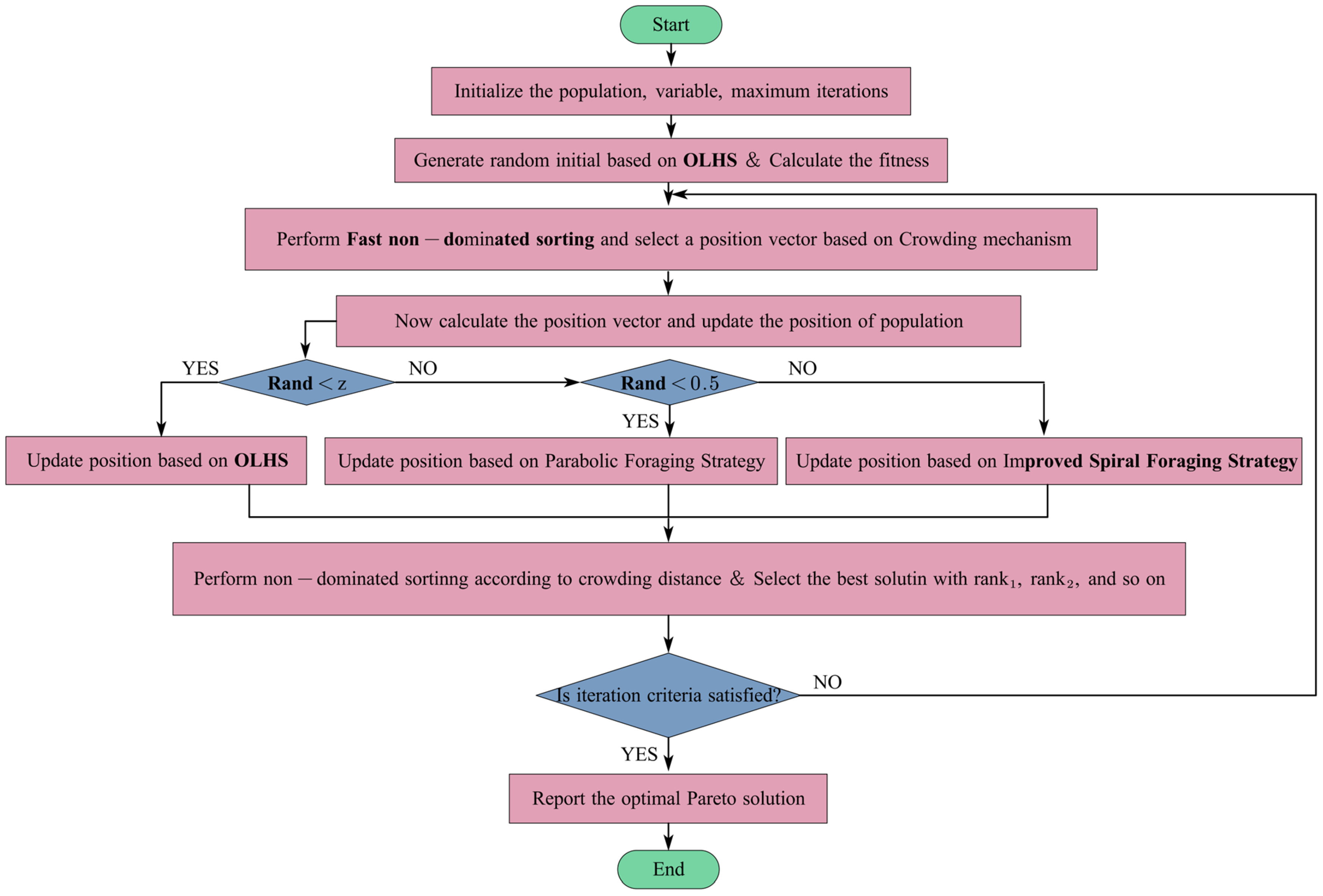
2.5. Basic Work of the FNS-TSO Algorithm

The operational framework of the FNS-TSO algorithm is structured into four phases: Phase 1: The tuna population is initialized, and the fitness of the tuna swarm positions is calculated based on the objective function. Phase 2: The positions of the tuna swarms are updated through spiral or parabolic motion patterns. With equal probability (50%), the swarm follows either a spiral or parabolic path during optimization, thereby determining the next candidate positions. Phase 3: The FNS-TSO algorithm maintains the best Pareto solutions in an archive and allows dynamic adjustment of solutions during iterations. If the archive reaches capacity (exceeding a user-defined threshold), non-dominated solutions with larger crowding distances are selectively retained based on the crowding distance mechanism. Phase 4: Iteration termination: The search systematically terminates in uncertain search spaces when the maximum iteration threshold enforces convergence to the optimum. The FNS-TSO workflow is illustrated in Figure 7.

3. Analysis of Test Function Results

3.1. Test Functions and Algorithm Parameters

To validate the performance of the FNS-TSO algorithm, it was tested on nine different multi-objective functions, including seven 2-objective test functions (ZDT1, ZDT2, ZDT3, ZDT4, ZDT6, Schaffer, and Kursawe) and two 3-objective test functions (Viennet2 and Viennet3). Test functions such as the ZDT series, Schaffer function, and Viennet series are core tools for optimization algorithm validation due to their standardized design, diversity of challenge coverage (e.g., multimodal landscapes, non-convex fronts, conflicting objectives), and scalability. Algorithms such as MOPSO, NSGA-II, and MOJSO were also tested to analyze their performance in generating diverse Pareto fronts. See Appendix A.2 for details of the test functions.
Each algorithm was run independently 30 times. And the parameters of the FNS-TSO, MOPSO, MOJSO, and NSGA-II algorithms are shown in Table 1. The setting of relevant parameters is based on the literature and practical experience. The test conditions of the algorithms are set as follows: M a x i t e r = 100 is the maximum number of iterations, N p o p = 150 is the number of populations, and N r = 200 is the archive size. c is the coefficient that controls the movement of the tuna swarm to its optimal or previous position; z is the probability that the FNS-TSO randomly performs the Optimal Latin hypercube initialization. When the value of c is large, the tuna population tends to swim to the optimal position and the results obtained will be more accurate; the smaller the value of z , the smaller the probability that the population will undergo initialization and the better the performance of the iteration. s max and s min are control parameters that control the rate of change of the weights.

3.2. Evaluation Metrics for Algorithms

Regarding performance metrics, we employ evaluation indicators including Inverted Generational Distance (IGD) [40], Hypervolume (HV) [41], and Spacing (SP) [17,42] to compare algorithmic convergence and robustness among different methods.
The Inverted Generational Distance (IGD) represents the average distance from each reference point to the nearest solution. A smaller IGD value indicates better algorithm convergence and diversity, and its mathematical expression is expressed as follows:
I G D = i = 1 n d i 2 n
Specific explanations are provided in Appendix A.1.
The Hypervolume (HV) represents the volume of the region in the objective space enclosed by the set of non-dominated solutions generated by the algorithm and a reference point. A higher HV value indicates broader coverage of the algorithm’s solution set, as well as superior overall performance; its mathematical expression is:
H V = δ ( i = 1 S v i )
Specific explanations are provided in Appendix A.1.
The Spacing (SP) metric quantifies the standard deviation of minimum distances between each solution and all other solutions in the set. A lower SP value corresponds to a more uniform distribution of globally optimal non-dominated solutions, with its mathematical formulation expressed as:
S P = 1 m 1 i = 1 m d ¯ d i 2
d i = min j ( f 1 i ( x ) f 1 j ( x ) + f 2 i ( x ) f 2 j ( x ) ) , i , j = 1 , 2 , , n
Specific explanations are provided in Appendix A.1.
The performance test results of IDG, HV, and SP on ZDT-series test functions, including Schaffer, Kursawe, Viennet2, and Viennet3, are shown in Figure 8, Figure 9, Figure 10, Figure 11, Figure 12, Figure 13, Figure 14, Figure 15 and Figure 16. Among them, Figure 8, Figure 11 and Figure 14 show the maximum values of the evaluation metrics; Figure 9, Figure 12 and Figure 15 show the minimum values of the evaluation metrics; and Figure 10, Figure 13 and Figure 16 show the average values of the evaluation metrics.

3.2.1. Analysis of Results for IGD

As shown in Figure 8, Figure 9 and Figure 10, the IGD metric of FNS-TSO achieves the lowest values on test functions ZDT1, ZDT2, ZDT3, ZDT4, Schaffer, Kursawe, Viennet2, and Viennet3, with average reductions of 49.13%, 32.22%, 53.51%, 98.49%, 8.74%, 28.70%, 14.00%, and 39.98% compared to the suboptimal algorithm. In ZDT6 test results, FNS-TSO’s average IGD value was higher than only MOPSO (2.54 times MOPSO’s average) but exhibited 55.96% and 93.33% lower IGD values than MOJSO and NSGA-II, respectively. MOPSO demonstrated superior performance in the ZDT6 test. These IGD comparisons indicate that FNS-TSO outperforms other algorithms in both convergence and diversity.

3.2.2. Analysis of Results for HV

As shown in Figure 11, Figure 12 and Figure 13, FNS-TSO achieved the highest Hypervolume (HV) values on test functions ZDT1, ZDT4, and Schaffer, exceeding suboptimal results by factors of 1.0033, 1.0114, and 1.005, respectively. For minimum HV metrics, FNS-TSO demonstrated superiority on ZDT1, ZDT3, ZDT4, Schaffer, and Viennet3, outperforming suboptimal algorithms by 1.0110, 1.0131, 5.2603, 1.0006, and 1.0006 times, respectively. Regarding average HV performance, FNS-TSO attained optimal values on ZDT1, ZDT4, Schaffer, and Viennet3, surpassing suboptimal solutions by 1.0103, 1.9729, 1.0003, and 1.0005 times, respectively. Conversely, suboptimal performance was observed for ZDT2 and ZDT3, with HV values 0.36% and 0.123% lower than the optimal algorithm. These HV metric comparisons conclusively demonstrate FNS-TSO’s overall performance advantage over competing algorithms.

3.2.3. Analysis of Results for SP

From Figure 14, Figure 15 and Figure 16, the data demonstrate that the SP metric of FNS-TSO achieves the lowest values on test functions ZDT1, ZDT2, ZDT3, ZDT4, Kursawe, Viennet2, and Viennet3, with average values 41.25%, 38.41%, 32.44%, 51.14%, 58.80%, 9.92%, and 24.68% lower than suboptimal algorithms, respectively. On the Schaffer test function, although FNS-TSO’s minimum SP value represents a suboptimal result (1.03× the optimal algorithm’s value), its average value remains superior, outperforming the suboptimal algorithm by 9.40%. These results indicate that FNS-TSO exhibits superior convergence across multiple benchmark functions. However, FNS-TSO underperformed in the ZDT6 test, exhibiting an average value 2.33× higher than the optimal algorithm, where MOJSO demonstrated the best performance. SP metric analysis confirms that FNS-TSO’s solution set demonstrates both enhanced uniformity and strong convergence characteristics.

3.3. Stability Analysis

In this paper, to validate that the performance differences among the algorithms are inherent rather than caused by random errors, the variance and standard deviation of the FNS-TSO algorithm for individual evaluation metrics are calculated to assess algorithmic stability and robustness. Comparative variance plots of the MOJSO, MOPSO, NSGA-II, and FNS-TSO algorithms are generated to verify the stability of the experimental data.
The variance and standard deviation of each evaluation metric (IGD, HV, SP) for the FNS-TSO algorithm are shown in Table 2 and Table 3. The data reveal that both the variance (with magnitudes ranging from 1 × 10⁻¹⁰ to 1 × 10⁻³) and the standard deviation (with magnitudes ranging from 1 × 10⁻⁵ to 1 × 10⁻²) are significantly small. This indicates minimal data variability and stable results with high algorithmic robustness.
Figure 17, Figure 18 and Figure 19 show the variance comparison of evaluation results for the MOJSO, MOPSO, NSGA-II, and FNS-TSO algorithms. From the graphs, it can be observed that among the test functions used in this study, only ZDT4 and ZDT6 exhibit minor fluctuations, with HV and SP fluctuations at the 1 × 10⁻² order of magnitude. Notably, only the MOJSO algorithm in Figure 17 showed significant fluctuations in the ZDT6 function test results. Overall, the test results of these four optimization algorithms demonstrate high stability.

3.4. Pareto Front Analysis of Algorithms

From Figure 20, Figure 21, Figure 22, Figure 23, Figure 24, Figure 25, Figure 26, Figure 27 and Figure 28, it can be observed that the FNS-TSO algorithm exhibits superior convergence performance in the ZDT1, ZDT2, ZDT3, ZDT4, Schaffer, Kursawe, Viennet2, and Viennet3 test functions but demonstrates inferior convergence in the ZDT6 benchmark.
As shown in Figure 20 and Figure 21, the test results for ZDT1 and ZDT2 demonstrate that the solution sets of FNS-TSO and MOJSO are closer to the true Pareto front. However, the FNS-TSO solution set exhibits a more uniform distribution compared to MOJSO, with almost all solutions lying precisely on the true Pareto front. In contrast, a small portion of MOJSO’s solutions deviate from this front. The MOPSO solution set initially appears to align with the true Pareto front, but close inspection (see zoomed regions) reveals noticeable deviations. Similarly, the NSGA-II solution set shows a significant deviation from the true Pareto front.
As shown in Figure 22, both FNS-TSO and MOPSO solution sets are close to the true Pareto front in the ZDT3 test results. However, the FNS-TSO solution set demonstrates a more uniform distribution and nearly aligns completely with the true Pareto front, whereas the MOPSO solution set appears to follow the front initially but deviates upon closer inspection, as evidenced by the magnified view. In contrast, the MOJSO solution set exhibits a non-uniform distribution with some solutions straying from the true Pareto front, while the NSGA-II solution set shows significant deviation from the front.
As shown in Figure 23 regarding the ZDT4 test results, both FNS-TSO and MOJSO solution sets approach the true Pareto front, with FNS-TSO demonstrating superior distribution uniformity compared to MOJSO; while FNS-TSO’s solution set is almost entirely located on the true Pareto front, several solutions in MOJSO’s solution set exhibit deviations from the true Pareto front. Furthermore, both the MOPSO and NSGA-II solution sets significantly diverge from the true Pareto front.
As shown in Figure 24, the convergence performance of FNS-TSO, MOJSO, MOPSO, and NSGA-II is suboptimal in ZDT6 benchmark tests. However, a small subset of solutions in the MOJSO and MOPSO solution sets lie precisely on the true Pareto front, whereas the solution sets of FNS-TSO and NSGA-II exhibit significant deviations from the true Pareto front.
As shown in Figure 25, in the Kursawe test results, the solution sets of FNS-TSO and NSGA-II are close to the true Pareto front. However, the FNS-TSO solution set demonstrates superior uniformity and nearly coincides with the true Pareto front compared to NSGA-II. The zoomed-in view reveals that a small subset of NSGA-II solutions deviates from the true Pareto front. In contrast, MOPSO and MOJSO exhibit non-uniform distribution with significant deviations from the true Pareto frontier.
As shown in Figure 26, in tests on the Schaffer function, the FNS-TSO, MOJSO, MOPSO, and NSGA-II algorithms all demonstrate strong convergence performance, with solution sets exhibiting even distribution across the true Pareto-optimal front.
As shown in Figure 27 and Figure 28, the FNS-TSO solution sets consistently converge to the true Pareto front with uniform distribution in the Viennet2 and Viennet3 test results. In contrast, MOJSO, MOPSO, and NSGA-II exhibit partial solution deviations from the Pareto front and non-uniform distribution patterns.
In summary, the FNS-TSO algorithm demonstrates strong agreement in both IGD and SP evaluation metrics, achieving optimal test results across the ZDT1, ZDT2, ZDT3, ZDT4, Schaffer, Kursawe, Viennet2, and Viennet3 test functions. Notably, it also attains optimal HV metric performance in most test functions. The solution sets generated by FNS-TSO for these benchmark functions exhibit closer proximity to the true Pareto front with more uniform distribution patterns. This empirically validates the algorithm’s superior convergence, robustness, and stable performance under variations in problem parameters or constraint conditions. These characteristics collectively indicate the comprehensive performance advantages of FNS-TSO.

4. Application of FNS-TSO in Underwater Manipulator Trajectory Optimization Problem

Underwater manipulators require smooth and stable operation to perform tasks such as grasping and exploration. When meeting impact constraints, it is essential to optimize the operational duration and energy consumption of underwater manipulators to improve work efficiency and reduce energy costs. Therefore, this paper establishes a trajectory model using quintic spline interpolation with three optimization objectives: total time, total energy consumption, and total impact for underwater manipulators. The FNS-TSO algorithm is then applied to perform trajectory optimization and obtain the Pareto optimal solution set.
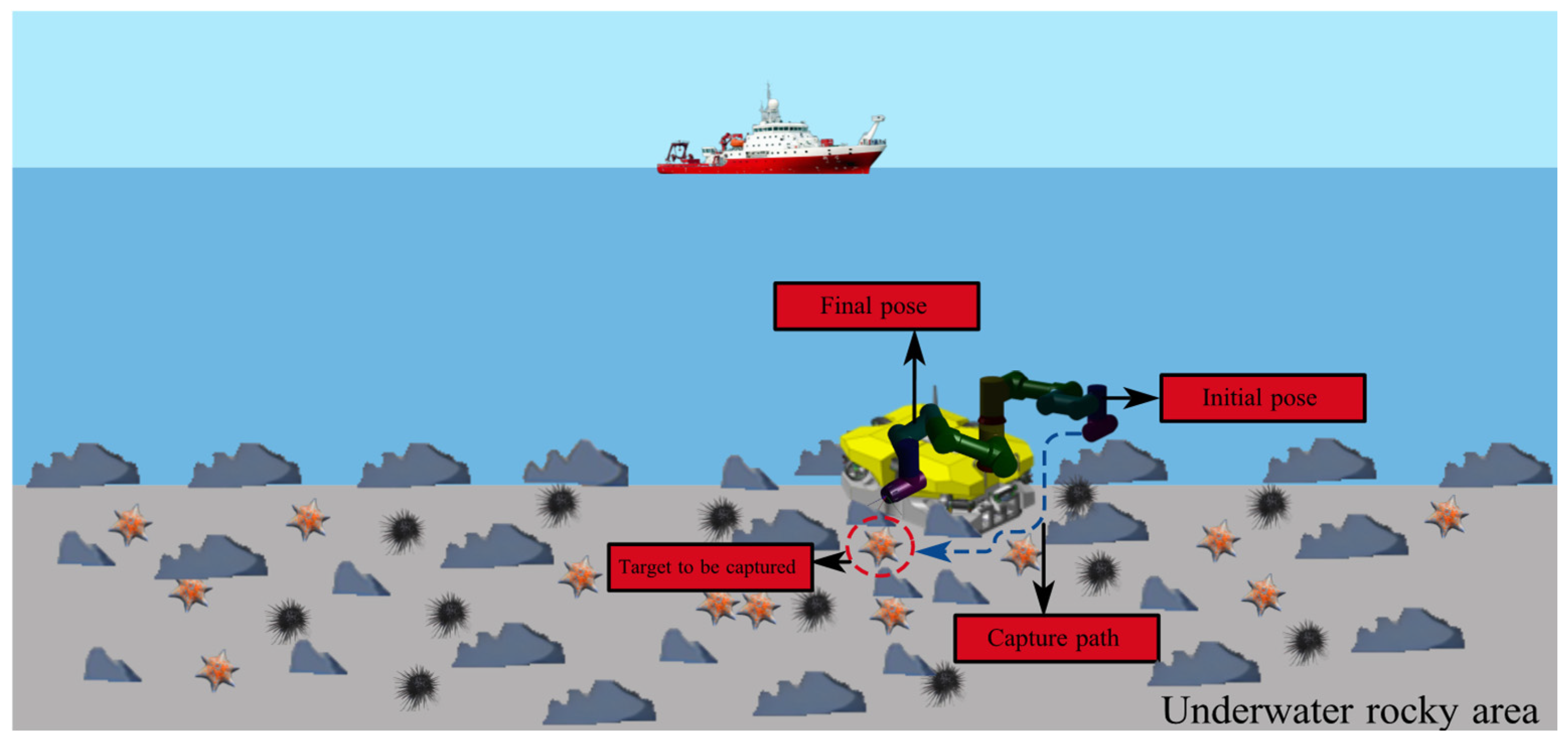
Our underwater manipulator is primarily employed for tasks such as underwater mineral collection and marine biological sample capture. As shown in Figure 29, the underwater manipulator needs to complete point-to-point movement from the end of the arm to the object being grabbed during the task. Multiple path points can be selected between the starting and ending points, resulting in numerous potential paths traversing these points. It is necessary to choose the optimal path that achieves the time-energy-impact optimization. The optimal time aims to improve work efficiency and enable the acquisition of more mineral resources within a limited timeframe; the electric-driven manipulator can only carry a limited battery capacity during operation, and thus the optimal energy consumption addresses the limited energy capacity and the optimal impact ensures smoother operation.

4.1. Derivation of Quintic Spline Interpolation

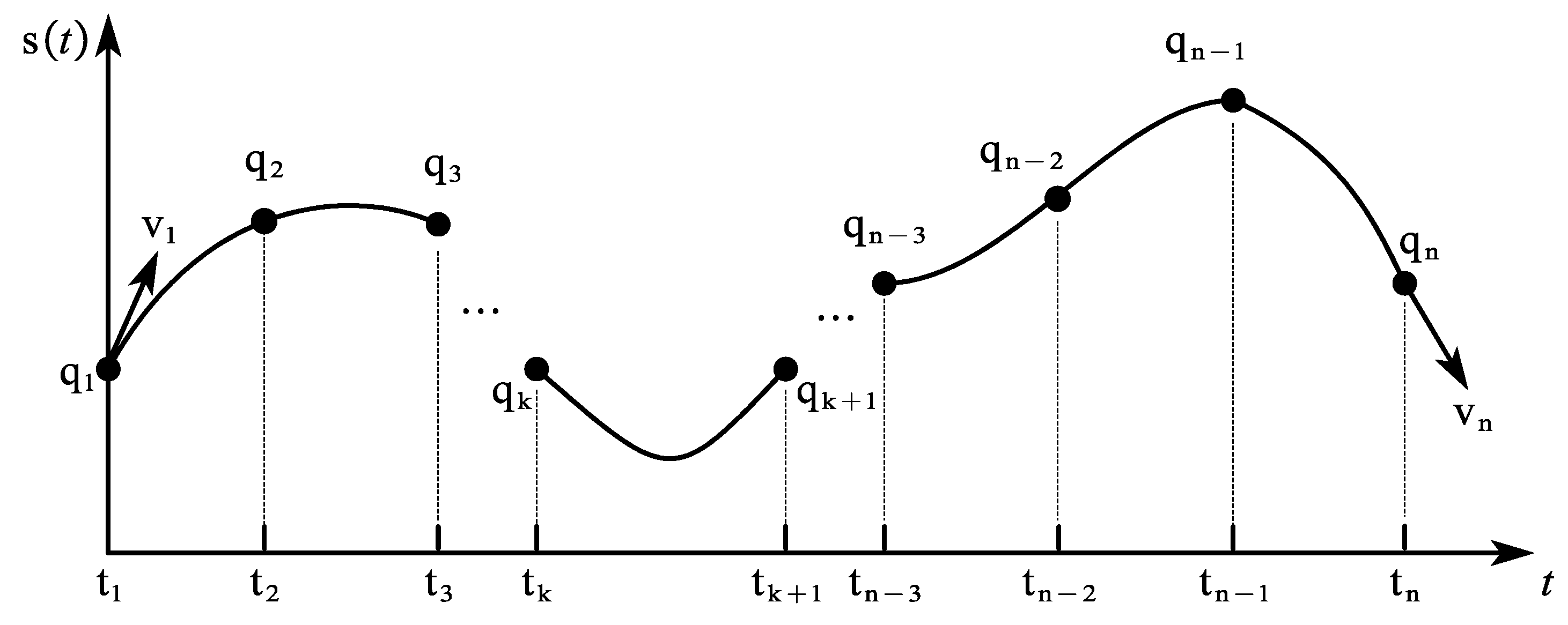
When given n points, instead of using a single quintic interpolating polynomial, we can employ n − 1 quintic polynomials, each defining a trajectory segment. The resulting composite function s(t) is called a fifth-order spline curve. Quintic spline interpolation ensures both smooth and continuous transitions of velocity and acceleration at all interpolation points while also guaranteeing zero initial and final velocities and accelerations in the planned trajectory. This significantly mitigates the start–stop shock in underwater manipulators.
Define the functional form of a quintic spline curve as:
s t = q k t , t t k , t k + 1 , k = 1 , , n 1 q k t = a k + b k t t k + c k t t k 2 + d k t t k 3 + e k t t k 4 + f k t t k 5
This trajectory consists of n − 1 quintic polynomials and each polynomial requires the computation of six parameters, resulting in a total of 6n − 6 coefficients to be determined. As shown in Figure 30, the initial velocity is s ˙ t 1 = v 1 , the termination velocity is s ˙ t n = v n , and under natural conditions, the acceleration s ¨ t 1 and s ¨ t n at the initial and final moments are both 0. To ensure the smoothness of position, velocity, and acceleration and reduce the impact during motion, quintic spline interpolation needs to satisfy the continuity of s t , s t , s t , s 3 t , s 4 t .
q k t = a k + b k Δ t + c k Δ t 2 + d k Δ t 3 + e k Δ t 4 + f k Δ t 5 q k t = b k + 2 c k Δ t + 3 d k Δ t 2 + 4 e k Δ t 3 + 5 f k Δ t 4 q k t = 2 c k + 6 d k Δ t + 12 e k Δ t 2 + 20 f k Δ t 3 q k 3 t = 6 d k + 24 e k Δ t + 60 f k Δ t 2 q k 4 t = 24 e k + 120 f k Δ t
where Δ t = t t k .
From the interpolation condition:
q k t k = a k = y k
And the spline curve is continuous at each segment transition, i.e:
q k m t k + 1 = q k + 1 m t k + 1 , k = 1 , n 2 ; m = 1 , 2 , 3 , 4
Through deduction, the interpolation formula for the quintic spline is written in matrix form as:
1 2 λ 1 8 7 ω 1 λ 1 ω 1 λ 1 ω 1 μ 2 δ 2 λ 2 ω 2 j 1 λ 1 l 2 μ 2 j 2 λ 2 λ 2 ω 2 μ 3 δ 3 λ 3 ω 3 j 2 λ 2 l 3 μ 3 j 3 λ 3 λ n 2 ω n 2 μ n 1 δ n 1 λ n 1 ω n 1 j n 2 λ n 2 l n 1 μ n 1 j n 1 λ n 1 1 λ n 1 ω n 1 2 λ n 1 8 7 ω n 1 M 1 N 1 M 2 N 2 M 3 N 3 M n 1 N n 1 M n N n = β 1 y 2 y 1 T 1 ρ 1 τ 2 0 τ 3 0 τ n 1 0 β n ρ n y n y n 1 T n 1

4.2. Optimal Trajectory Planning Based on FNS-TSO

The decision variable for trajectory multi-objective optimization is the time length of each interpolation interval, denoted as Δ T = ( Δ T 1 , Δ T 2 , , Δ T n ) T , where Δ T i = t i + 1 t i , i = 1 , 2 , , n , t i denotes the time series of the trajectory points, and the time of the first point is t 1 , usually taken as t 1 = 0 . The defined optimization objective function and the constraints are shown below.
Objective function:
f 1 = i = 1 n Δ T i f 2 = i = 1 n 1 Δ T i 0 Δ T i A i 2 d t f 3 = i = 1 n 1 Δ T i 0 Δ T i J i 2 d t
where f 1 is the time optimum, n denotes the number of interpolation intervals, f 2 is the energy objective function, A i denotes the acceleration variable for each interval, f 3 is the objective function of the shock, and J i denotes the additive acceleration variable for each interpolation interval.
Constraints:
max v i v max max A i A max max J i J max
where v i and v max , respectively, denote the speed at which the i -th joint operates and the maximum joint speed allowed, A i and A max respectively denote the acceleration at which the i -th joint operates and the maximum joint acceleration allowed, and J i and J max denote the accelerated acceleration at which the i -th joint operates and the maximum joint accelerated acceleration allowed, respectively.
Assuming that the underwater manipulator needs to move along a curve L in Cartesian space to accomplish the task of handling minerals on the seafloor, the position parameters ( p x , p y , p z , α , β , γ ) of the passing points are as shown in Table 4.
Through the kinematic inverse solution, the angular interpolation points of the six joints were obtained, which are shown in Table 5.
The value range of the decision variables is Δ T i 0.01 , 5 , and the velocity and acceleration at the start and end points of the underwater manipulator are set to 0. The constraints are:
max v j v max = 80 / s max A j A max = 60 / s 2 max J j J max = 50 / s 3
The times for each interpolation interval for the underwater manipulator selected before optimization are shown in Table 6.
Based on the timings listed in the table, quintic spline interpolation is performed, and the motion parameters’ variation of each joint in the underwater manipulator is simulated using MATLAB(R2023b), as shown in Figure 31.
The simulation results show that the joint trajectories are smooth and continuous, with velocities and accelerations at the start and end being zero. However, during the initial movement phase, joints 2 and 3 exhibit excessive impact forces, while joints 2 and 4 demonstrate similar issues in the final phase, causing the joint jerk to exceed the specified threshold. Furthermore, parameters such as time, energy, and impact fail to reach optimal values.
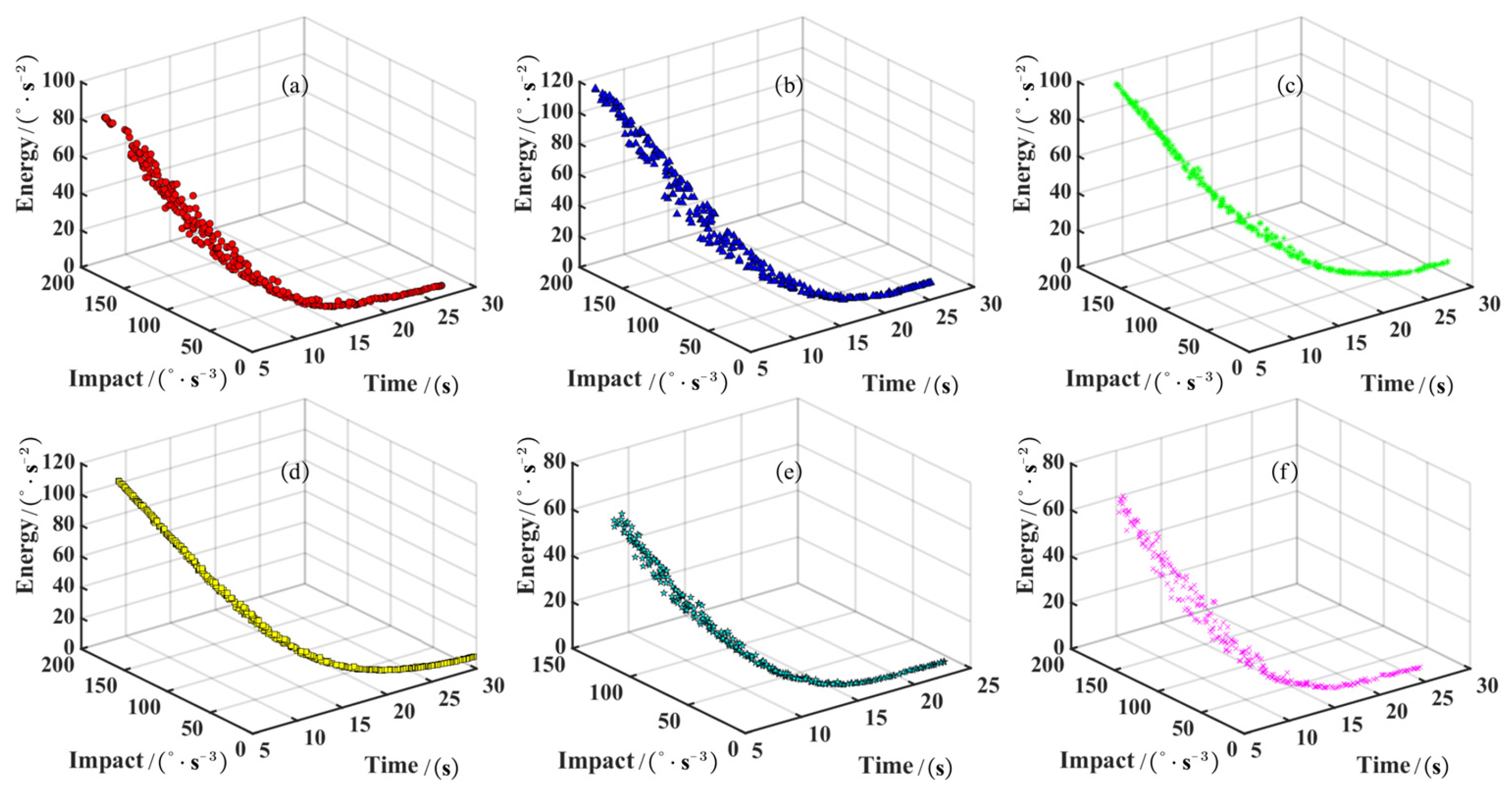
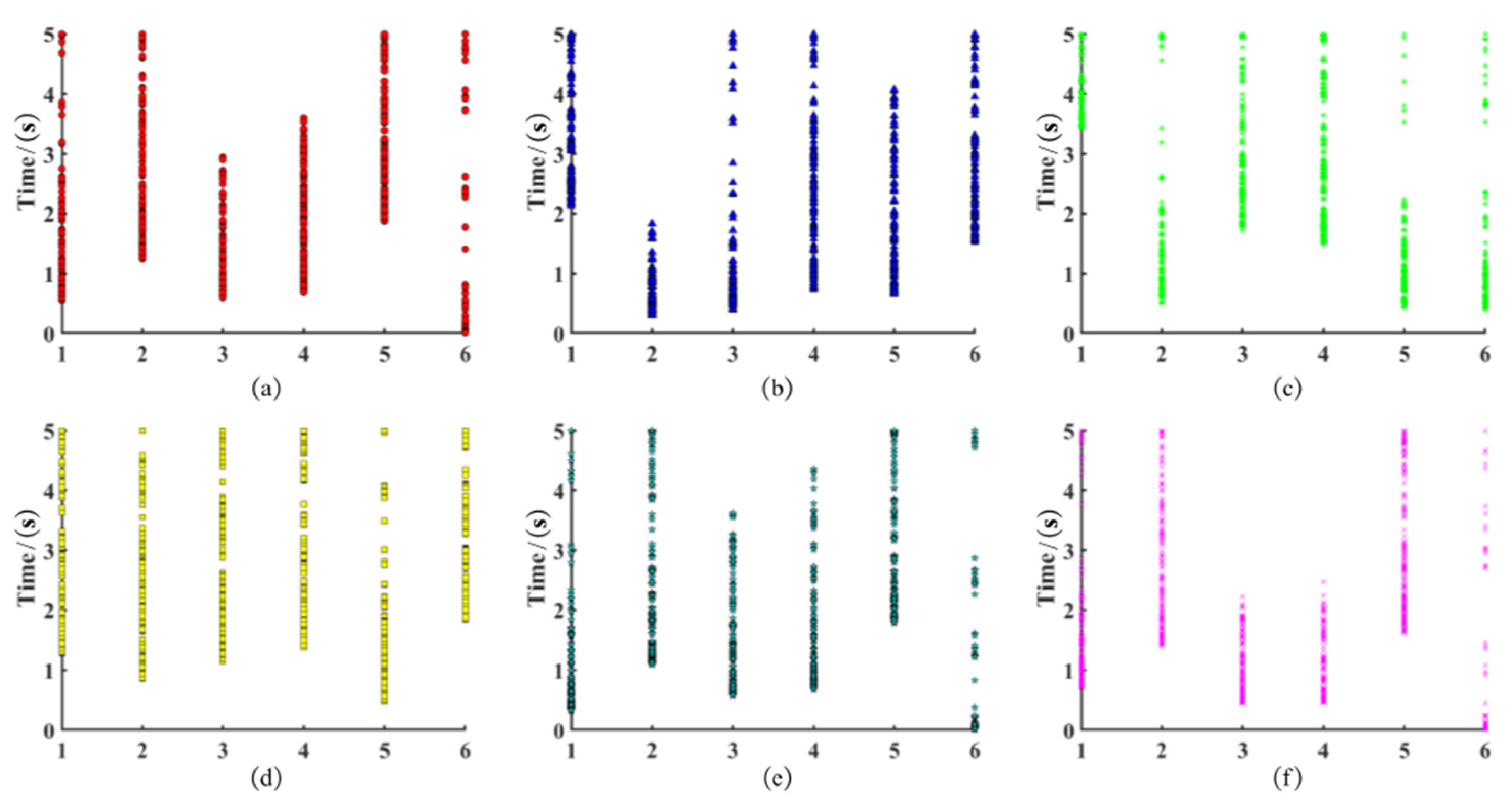
The FNS-TSO algorithm was applied to conduct multi-objective optimization for each joint of the underwater manipulator independently, with a population size and maximum iteration count of 300 each. This process generated the Pareto front and population distribution for each joint, as illustrated in Figure 32 (Pareto fronts) and Figure 33 (population distributions), respectively.
From the Pareto frontiers, analysis reveals an inverse relationship between time and energy consumption/impact: extended durations correspond to lower energy consumption and reduced impact, while shorter durations exhibit higher energy consumption and amplified impact. Therefore, engineering applications require selection based on actual operational constraints. This study prioritizes energy efficiency and impact mitigation, selecting a balanced time duration through multi-criteria analysis (see Table 7).
To ensure synchronized joint movements in underwater manipulators, the maximum joint movement time is selected for each segment of the interval, as detailed in Table 8.
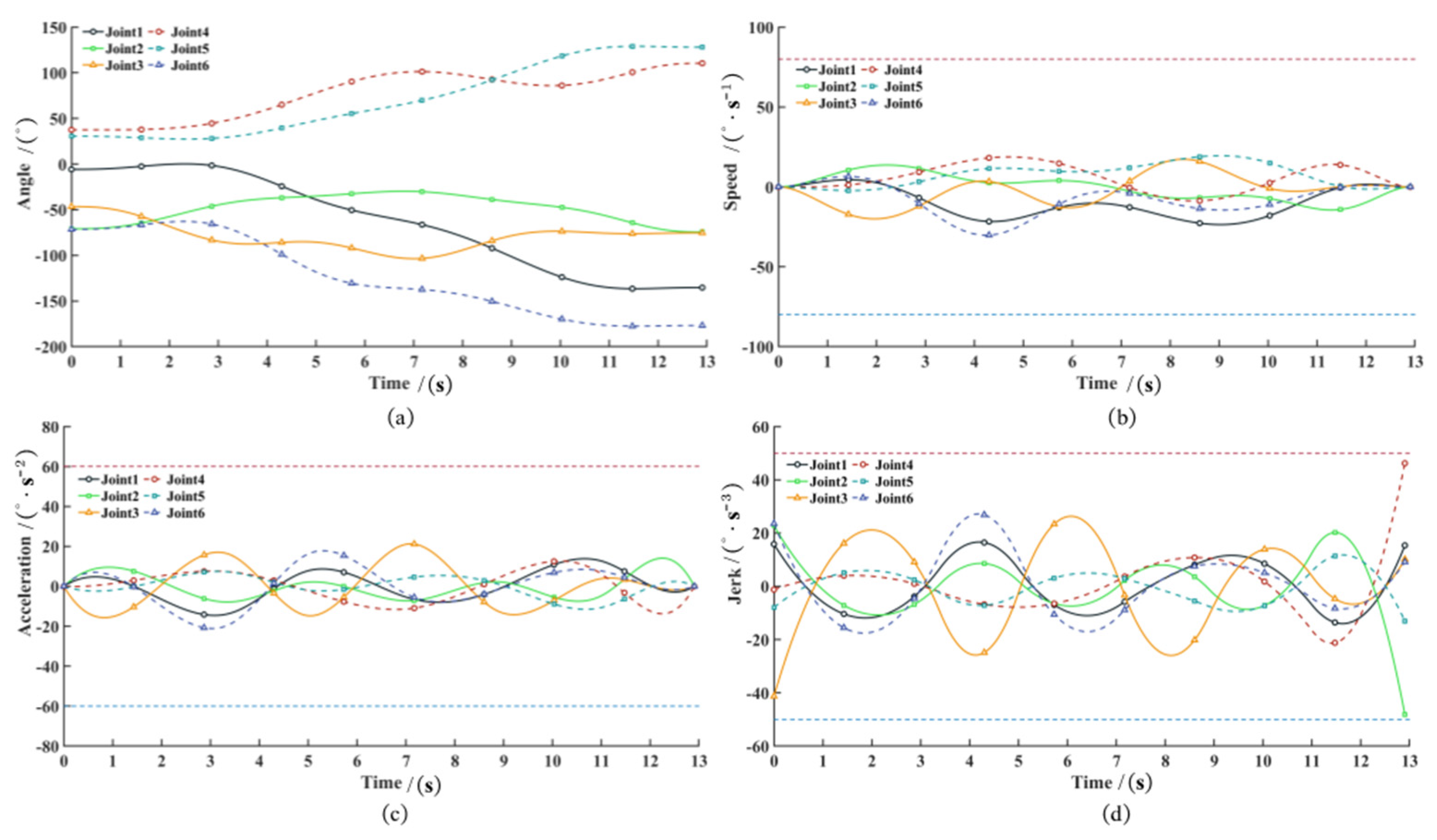
The variations in angle, angular velocity, angular acceleration, and jerk of the optimal quintic spline trajectories for each joint are shown in Figure 34.
The simulation results demonstrate that the optimally planned trajectory is smooth, continuous, and free of abrupt changes. The manipulator’s end-effector passes precisely through all predefined path points, while joint speed, acceleration, and jerk remain within constraint limits throughout the operation. The quintic spline trajectory fully satisfies all technical requirements. Quantitative comparisons of the underwater manipulator’s total operation time, total joint energy consumption, and impact before and after optimization are presented in Table 9.
The tabular data demonstrate that the manipulator’s total operation time decreases by 11.03%, with 19.02% reduction in energy consumption and 24.69% mitigation of total impact compared to pre-optimization benchmarks. The multi-objective optimized trajectory therefore ensures smooth underwater operation while enhancing efficiency and significantly reducing energy expenditure.

5. Conclusions

This study proposes a Fast Non-Dominated Sorting Tuna Swarm Optimization (FNS-TSO) algorithm. The initialization phase employs Optimal Latin Hypercube Sampling to enhance population uniformity, while a nonlinear dynamic weight mechanism refines the spiral foraging strategy, balancing exploration–exploitation tradeoffs to improve convergence and robustness. Comparative evaluations with MOPSO, MOJSO, and NSGA-II on two-objective and three-objective benchmark functions demonstrate FNS-TSO’s superior performance in convergence, solution diversity, and distribution uniformity. In its engineering application, the algorithm reduces underwater manipulator motion trajectory optimization outcomes by 11.03% (time), 19.02% (energy), and 24.69% (impact), validating its practical efficacy.
The future research work and current limitations of this article include:
  • The algorithm has only been validated for its effectiveness in trajectory optimization of underwater manipulators and has not been validated in other engineering fields.
  • Benchmark evaluations limited to ≤3 objectives, leaving scalability to higher-dimensional problems unverified
These constraints highlight critical research directions for multi-objective optimization algorithm development.

Author Contributions

Conceptualization, X.W.; methodology, X.W.; software, X.W.; writing—original draft preparation, X.W.; writing—review and editing, G.X., S.H. and Y.L.; visualization, X.W. and F.B.; supervision, Y.L.; project administration, Y.L.; funding acquisition, Y.L. All authors have read and agreed to the published version of the manuscript.

Funding

This research was funded by the Marine Carbon Sink and Biogeochemical Process Research Center, National Natural Science Foundation of China, grant number No. 42188102 and No. 52201328, the National Key Research and Development Program of China, grant number No. 2023YFC2810100 and No. 2023YFB4204103.

Data Availability Statement

Data available on request due to restrictions. The data presented in this study are available on request from the corresponding author due to laboratory management requirements.

Conflicts of Interest

The authors declare no conflicts of interest.

Appendix A

Appendix A.1

Table A1. Nomenclature.
NumberParameter
Symbols
Specific Annotations
1 X i k The level of factor k on the i -th run
2 u i k The independent random variables U 0 , 1 )
3 d ( x i , x j ) The distance between two sample points x i and x j
4 n The number of true Pareto-optimal solutions
5 d i The Euclidean distance between the i-th true Pareto-optimal solution in the reference set and the most recently obtained Pareto-optimal solution
6 δ The Lebesgue measure, which is used to measure the volume
7 S The number of nondominated solution sets
8 v i The hypervolume constituted by the reference point and the i -th solution in the solution set
9 d ¯ The average of all d i
10 m The number of Pareto-optimal solutions

Appendix A.2

Table A2. Test function parameters.
ProblemVariable
Bounds
Objective Functions
ZDT1 0 , 1 f 1 ( x ) = x 1
f 2 ( x ) = g ( x ) 1 x 1 / g ( x )
g ( x ) = 1 + 9 ( i = 2 n x i ) / ( n 1 )
ZDT2 0 , 1 f 1 ( x ) = x 1
f 2 ( x ) = g ( x ) 1 ( x 1 / g ( x ) ) 2
g ( x ) = 1 + 9 ( i = 2 n x i ) / ( n 1 )
ZDT3 0 , 1 f 1 ( x ) = x 1
f 2 ( x ) = g ( x ) 1 x 1 / g ( x ) ( x 1 / g ( x ) ) sin ( 10 π x 1 )
g ( x ) = 1 + 9 ( i = 2 n x i ) / ( n 1 )
ZDT4 0 , 1 f 1 ( x ) = x 1
f 2 ( x ) = g ( x ) 1 x 1 / g ( x ) ( x 1 / g ( x ) ) sin ( 10 π x 1 )
g ( x ) = 1 + 9 ( i = 2 n x i ) / ( n 1 )
ZDT6 0 , 1 f 1 ( x ) = 1 exp ( 4 x 1 ) sin 6 ( 6 π x 1 )
f 2 ( x ) = g ( x ) 1 ( f 1 ( x ) / g ( x ) ) 2
g ( x ) = 1 + 9 ( i = 2 n x i ) / ( n 1 ) 0.25
Schaffer x i 5 , 5 , i = 1 , 2 f ( x 1 , x 2 ) = 0.5 ( sin 2 ( x 1 2 + x 2 2 ) 0.5 ) ( 1 + 0.001 ( x 1 2 + x 2 2 ) ) 2
Kursawe x i 5 , 5
i 1 , 3
f 1 ( x ) = i = 1 2 10 exp ( 0.2 x i 2 + x i + 1 2 )
f 2 ( x ) = i = 1 2 x i 0.8 + 5 sin ( x i 3 )
Viennet2 x 1 4 , 4
x 2 4 , 4
f 1 ( x ) = 0.5 ( x 1 2 ) 2 + ( x 2 + 1 ) 2 13 + 3
f 2 ( x ) = ( x 1 + x 2 3 ) 2 36 + ( x 1 + x 2 + 2 ) 2 8 17
f 3 ( x ) = ( x 1 + 2 x 2 1 ) 2 175 + ( 2 x 2 x 1 ) 2 17 13
Viennet3 x 1 3 , 10
x 2 10 , 3
f 1 ( x ) = 0.5 ( x 1 2 + x 2 2 ) + sin ( x 1 2 + x 2 2 )
f 2 ( x ) = ( 3 x 1 2 x 2 + 4 ) 2 8 + ( x 1 x 2 + 1 ) 2 27 + 15
f 3 ( x ) = 1 / ( x 1 2 + x 2 2 + 1 ) 1.1 × e ( ( x 1 2 + x 2 2 ) )

References

  1. Kelley, C.T. Detection and remediation of stagnation in the Nelder–Mead algorithm using a sufficient decrease condition. SIAM J. Optim. 1999, 10, 43–55. [Google Scholar] [CrossRef]
  2. Vogl, T.P.; Mangis, J.K.; Rigler, A.K.; Zink, W.T.; Alkon, D.L. Accelerating the convergence of the back-propagation method. Biol. Cybern. 1988, 59, 257–263. [Google Scholar] [CrossRef]
  3. Wu, G.; Pedrycz, W.; Suganthan, P.N.; Mallipeddi, R. A variable reduction strategy for evolutionary algorithms handling equality constraints. Appl. Soft Comput. 2015, 37, 774–786. [Google Scholar] [CrossRef]
  4. Wu, G. Across neighborhood search for numerical optimization. Inf. Sci. 2016, 329, 597–618. [Google Scholar] [CrossRef]
  5. Hare, W.; Nutini, J.; Tesfamariam, S. A survey of non-gradient optimization methods in structural engineering. Adv. Eng. Softw. 2013, 59, 19–28. [Google Scholar] [CrossRef]
  6. Holland, J.H. Genetic algorithms. Sci. Am. 1992, 267, 66–73. [Google Scholar] [CrossRef]
  7. Kirkpatrick, S.; Gelatt, C.D.; Vecchi, M.P. Optimization by simulated annealing. Science 1983, 220, 671–680. [Google Scholar] [CrossRef]
  8. Kennedy, J.; Eberhart, R. Particle swarm optimization. In Proceedings of the ICNN’95—International Conference on Neural Networks, Perth, WA, Australia, 27 November–1 December 1995; Volume 4, pp. 1942–1948. [Google Scholar] [CrossRef]
  9. Dorigo, M.; Birattari, M.; Stutzle, T. Ant colony optimization. IEEE Comput. Intell. Mag. 2006, 1, 28–39. [Google Scholar] [CrossRef]
  10. Gandomi, A.H.; Alavi, A.H. Krill Herd: A new bio-inspired optimization algorithm. Commun. Nonlinear Sci. Numer. Simul. 2012, 17, 4831–4845. [Google Scholar] [CrossRef]
  11. Mirjalili, S.; Mirjalili, S.M.; Lewis, A. Grey Wolf Optimizer. Adv. Eng. Softw. 2014, 69, 46–61. [Google Scholar] [CrossRef]
  12. Mirjalili, S.; Lewis, A. The Whale Optimization Algorithm. Adv. Eng. Softw. 2016, 95, 51–67. [Google Scholar] [CrossRef]
  13. Xie, L.; Han, T.; Zhou, H.; Zhang, Z.; Han, B.; Tang, A. Tuna Swarm Optimization: A Novel Swarm-Based Metaheuristic Algorithm for Global Optimization. Comput. Intell. Neurosci. 2021, 2021, 9210050. [Google Scholar] [CrossRef]
  14. Amiri, M.H.; Hashjin, N.M.; Montazeri, M.; Mirjalili, S.; Khodadadi, N. Hippopotamus optimization algorithm: A novel nature-inspired optimization algorithm. Sci. Rep. 2024, 14, 5032. [Google Scholar] [CrossRef] [PubMed]
  15. Tang, A.; Han, T.; Zhou, H.; Xie, L. An improved equilibrium optimizer with application in unmanned aerial vehicle path planning. Sensors 2021, 21, 1814. [Google Scholar] [CrossRef] [PubMed]
  16. Coello Coello, C.A.; Lechuga, M.S. MOPSO: A proposal for multiple objective particle swarm optimization. In Proceedings of the 2002 Congress on Evolutionary Computation, CEC’02 (Cat. No. 02TH8600), Honolulu, HI, USA, 12–17 May 2002; Volume 2, pp. 1051–1056. [Google Scholar] [CrossRef]
  17. Coello Coello, C.A.; Pulido, G.T.; Lechuga, M.S. Handling multiple objectives with particle swarm optimization. IEEE Trans. Evol. Comput. 2004, 8, 256–279. [Google Scholar] [CrossRef]
  18. Srinivas, N.; Deb, K. Muiltiobjective Optimization Using Nondominated Sorting in Genetic Algorithms. Evol. Comput. 1994, 2, 221–248. [Google Scholar] [CrossRef]
  19. Deb, K.; Agrawal, S.; Pratap, A.; Meyarivan, T. A fast elitist non-dominated sorting genetic algorithm for multi-objective optimization: NSGA-II. Parallel Probl. Solving Nat. PPSN VI 2000, 1917, 849–858. [Google Scholar] [CrossRef]
  20. Mirjalili, S.; Saremi, S.; Mirjalili, S.M.; Coelho, L.S. Multi-objective grey wolf optimizer: A novel algorithm for multi-criterion optimization. Expert Syst. Appl. 2016, 47, 106–119. [Google Scholar] [CrossRef]
  21. Jangir, P.; Jangir, N. Non-dominated sorting whale optimization algorithm (NSWOA): A multi-objective optimization algorithm for solving engineering design problems. Glob. J. Res. Eng. 2017, 17, 15–42. [Google Scholar]
  22. Aziz, M.A.E.; Ewees, A.A.; Hassanien, A.E. Multi-objective whale optimization algorithm for content-based image retrieval. Multimed. Tools Appl. 2018, 77, 26135–26172. [Google Scholar] [CrossRef]
  23. Jangir, P.; Jangir, N. A new Non-Dominated Sorting Grey Wolf Optimizer (NS-GWO) algorithm: Development and application to solve engineering designs and economic constrained emission dispatch problem with integration of wind power. Eng. Appl. Artif. Intell. 2018, 72, 449–467. [Google Scholar] [CrossRef]
  24. Chou, J.S.; Truong, D.N. Multiobjective optimization inspired by behavior of jellyfish for solving structural design problems. Chaos Solitons Fractals 2020, 135, 109738. [Google Scholar] [CrossRef]
  25. Li, L.; Ji, B.; Lim, M.K.; Tseng, M.L. Active distribution network operational optimization problem: A multi-objective tuna swarm optimization model. Appl. Soft Comput. 2024, 150, 111087. [Google Scholar] [CrossRef]
  26. Wolpert, D.H.; Macready, W.G. No free lunch theorems for optimization. IEEE Trans. Evol. Comput. 1997, 1, 67–82. [Google Scholar] [CrossRef]
  27. Huang, P.; Liu, G.; Yuan, J.; Xu, Y. Multi-objective optimal trajectory planning of space robot using particle swarm optimization. Int. Symp. Neural Netw. 2008, 5264, 171–179. [Google Scholar] [CrossRef]
  28. Marcos, M.G.; Tenreiro Machado, J.A.; Azevedo-Perdicoúlis, T.P. A multi-objective approach for the motion planning of redundant manipulators. Appl. Soft Comput. 2012, 12, 589–599. [Google Scholar] [CrossRef]
  29. Zhou, M.; Zhou, M.; Liu, G.; Chen, C. Time Optimal Trajectory Planning of Manipulator Based on Improved Butterfly Algorithm. Comput. Sci. 2023, 50, 220900284–220900292. [Google Scholar]
  30. Yang, D.; Zhao, Z.; Li, Z. Research on the trajectory planning of mechanical arm based on MPA. Mach. Des. Manuf. Eng. 2024, 53, 55–58. [Google Scholar] [CrossRef]
  31. Saravanan, R.; Ramabalan, S.; Balamurugan, C.; Subash, A. Evolutionary trajectory planning for an industrial robot. Int. J. Autom. Comput. 2010, 7, 190–198. [Google Scholar] [CrossRef]
  32. Huang, J.; Hu, P.; Wu, K.; Zeng, M. Optimal time-jerk trajectory planning for industrial robots. Mech. Mach. Theory 2018, 121, 530–544. [Google Scholar] [CrossRef]
  33. Wang, Z.; Li, Y.; Shuai, K.; Zhu, W.; Chen, B.; Chen, K. Multi-objective Trajectory Planning Method based on the Improved Elitist Non-dominated Sorting Genetic Algorithm. Chin. J. Mech. Eng. 2022, 35, 7. [Google Scholar] [CrossRef]
  34. Zhang, Y.; Di, H.; Chen, Z. Trajectory planning of manipulator based on NSGA-II under multi-objectives. Modul. Mach. Tool Autom. Manuf. Tech. 2024, 5, 65–70. [Google Scholar] [CrossRef]
  35. Tuerxun, W.; Xu, C.; Guo, H.; Guo, L.; Yin, L. Fault classification in wind turbine based on deep belief network optimized by modified tuna swarm optimization algorithm. J. Renew. Sustain. Energy 2022, 14, 033307. [Google Scholar] [CrossRef]
  36. Yan, Z.; Yan, J.; Wu, Y.; Cai, S.; Wang, H. A novel reinforcement learning based tuna swarm optimization algorithm for autonomous underwater vehicle path planning. Math. Comput. Simul. 2023, 209, 55–86. [Google Scholar] [CrossRef]
  37. Wang, Q.; Xu, M.; Hu, Z. Path Planning of Unmanned Aerial Vehicles Based on an Improved Bio-Inspired Tuna Swarm Optimization Algorithm. Biomimetics 2024, 9, 388. [Google Scholar] [CrossRef]
  38. Mckay, M.D.; Beckman, R.J.; Conover, W.J. A comparison of three methods for selecting values of output variables in the analysis of output from a computer code. Technometrics 1979, 21, 239–245. [Google Scholar]
  39. Johnson, M.E.; Moore, L.M.; Ylvisaker, D. Minimax and maximin distance designs. J. Stat. Plan. Inference 1990, 26, 131–148. [Google Scholar] [CrossRef]
  40. Sierra, M.R.; Coello Coello, C.A. Improving PSO-Based Multi-objective Optimization Using Crowding, Mutation and ∈-Dominance. In Evolutionary Multi-Criterion Optimization; Springer: Berlin/Heidelberg, Germany, 2005; Volume 3410. [Google Scholar] [CrossRef]
  41. Cai, X.; Xiao, Y.; Li, M.; Hu, H.; Ishibuchi, H.; Li, X. A Grid-Based Inverted Generational Distance for Multi/Many-Objective Optimization. IEEE Trans. Evol. Comput. 2021, 25, 21–34. [Google Scholar] [CrossRef]
  42. Schott, J.R. Fault Tolerant Design Using Single and Multicriteria Genetic Algorithm Optimization; Massachusetts Institute of Technology, Department of Aeronautics and Astronautics: Cambridge, MA, USA, 1995. [Google Scholar]
Figure 1. Latin Hypercube Sampling.
Jmse 13 00916 g001
Figure 2. Comparison of population distribution.
Jmse 13 00916 g002
Figure 3. Nonlinear dynamic weights.
Jmse 13 00916 g003
Figure 4. Non-dominated sorting.
Jmse 13 00916 g004
Figure 5. Crowding distance.
Jmse 13 00916 g005
Figure 6. Algorithm improvement.
Jmse 13 00916 g006
Figure 7. Flowchart of FNS-TSO algorithm.
Jmse 13 00916 g007
Figure 8. IGD (max) test results.
Jmse 13 00916 g008
Figure 9. IGD (min) test results.
Jmse 13 00916 g009
Figure 10. IGD (avg) test results.
Jmse 13 00916 g010
Figure 11. HV (max) test results.
Jmse 13 00916 g011
Figure 12. HV (min) test results.
Jmse 13 00916 g012
Figure 13. HV (avg) test results.
Jmse 13 00916 g013
Figure 14. SP (max) test results.
Jmse 13 00916 g014
Figure 15. SP (min) test results.
Jmse 13 00916 g015
Figure 16. SP (avg) test results.
Jmse 13 00916 g016
Figure 17. IGD variance comparison.
Jmse 13 00916 g017
Figure 18. HV variance comparison.
Jmse 13 00916 g018
Figure 19. SP variance comparison.
Jmse 13 00916 g019
Figure 20. ZDT1 Pareto front: (a) FNSTSO Pareto front; (b) MOPSO Pareto front; (c) MOJSO Pareto front; (d) NSGA2 Pareto front; (e) The Pareto front of all algorithms; (f) Partial enlarged image.
Jmse 13 00916 g020
Figure 21. ZDT2 Pareto front: (a) FNSTSO Pareto front; (b) MOPSO Pareto front; (c) MOJSO Pareto front; (d) NSGA2 Pareto front; (e) The Pareto front of all algorithms; (f) Partial enlarged image.
Jmse 13 00916 g021
Figure 22. ZDT3 Pareto front: (a) FNSTSO Pareto front; (b) MOPSO Pareto front; (c) MOJSO Pareto front; (d) NSGA2 Pareto front; (e) The Pareto front of all algorithms; (f) Partial enlarged image.
Jmse 13 00916 g022
Figure 23. ZDT4 Pareto front: (a) FNSTSO Pareto front; (b) MOPSO Pareto front; (c) MOJSO Pareto front; (d) NSGA2 Pareto front; (e) The Pareto front of all algorithms; (f) Partial enlarged image.
Jmse 13 00916 g023
Figure 24. ZDT6 Pareto front: (a) FNSTSO Pareto front; (b) MOPSO Pareto front; (c) MOJSO Pareto front; (d) NSGA2 Pareto front; (e) The Pareto front of all algorithms.
Jmse 13 00916 g024
Figure 25. Kursawe Pareto front: (a) FNSTSO Pareto front; (b) MOPSO Pareto front; (c) MOJSO Pareto front; (d) NSGA2 Pareto front; (e) The Pareto front of all algorithms; (f) Partial enlarged image.
Jmse 13 00916 g025
Figure 26. Schaffer Pareto front: (a) FNSTSO Pareto front; (b) MOPSO Pareto front; (c) MOJSO Pareto front; (d) NSGA2 Pareto front; (e) The Pareto front of all algorithms; (f) Partial enlarged image.
Jmse 13 00916 g026
Figure 27. Viennet2 Pareto front: (a) FNSTSO Pareto front; (b) MOPSO Pareto front; (c) MOJSO Pareto front; (d) NSGA2 Pareto front; (e) The Pareto front of all algorithms.
Jmse 13 00916 g027
Figure 28. Viennet3 Pareto front: (a) FNSTSO Pareto front; (b) MOPSO Pareto front; (c) MOJSO Pareto front; (d) NSGA2 Pareto front; (e) The Pareto front of all algorithms.
Jmse 13 00916 g028
Figure 29. Underwater manipulator gripping trajectory.
Jmse 13 00916 g029
Figure 30. Quintic spline interpolation.
Jmse 13 00916 g030
Figure 31. The change in motion parameters of each joint of the underwater manipulator before optimization: (a) Angle before optimization; (b) Speed before optimization; (c) Acceleration before optimization (d) Jerk before optimization.
Jmse 13 00916 g031
Figure 32. Pareto front of each joint of the manipulator: (a) Joint 1 Pareto front; (b) Joint 2 Pareto front; (c) Joint 3 Pareto front; (d) Joint 4 Pareto front; (e) Joint 5 Pareto front; (f) Joint 6 Pareto front.
Jmse 13 00916 g032
Figure 33. Population distribution of each joint of the manipulator: (a) Joint 1 population; (b) Joint 2 population; (c) Joint 3 population; (d) Joint 4 population; (e) Joint 5 population; (f) Joint 6 population.
Jmse 13 00916 g033
Figure 34. The change in motion parameters of each joint of the optimized underwater manipulator: (a) Optimized angle; (b) Optimized speed; (c) Optimized acceleration (d) Optimized jerk.
Jmse 13 00916 g034
Table 1. Algorithm parameter settings.
AlgorithmFNS-TSOMOPSOMOJSONSGA-II
Parameters M a x i t e r = 100 M a x i t e r = 100 M a x i t e r = 100 M a x i t e r = 100
N p o p = 150 N p o p = 150 N p o p = 150 N p o p = 150
N r = 200 N r = 200 N r = 200 N r = 200
c = 0.7 c 1 = 1 C 0 = 0.5 p c = 0.7
z = 0.05 c 2 = 2 p m u = 0.4
s max = 6 ω = 0.7 m u = 0.02
s min = 4 m u = 0.5 σ = 0.2
Table 2. Variance of evaluation metrics for FNS-TSO.
ZDT1ZDT2ZDT3ZDT4ZDT6SchafferKursaweVIennet2VIennet3
IGD7.29 × 10−71.65 × 10−63.56 × 10−71.92 × 10−83.62 × 10−33.91 × 10−71.10 × 10−66.72 × 10−72.99 × 10−7
HV1.50 × 10−68.82 × 10−62.24 × 10−61.18 × 10−71.61 × 10−31.30 × 10−81.24 × 10−69.46 × 10−88.84 × 10−10
SP1.77 × 10−73.60 × 10−71.47 × 10−51.48 × 10−76.91 × 10−31.88 × 10−61.34 × 10−67.27 × 10−71.02 × 10−5
Table 3. Standard deviation of evaluation metrics for FNS-TSO.
ZDT1ZDT2ZDT3ZDT4ZDT6SchafferKursaweVIennet2VIennet3
IGD8.54 × 10−41.28 × 10−35.96 × 10−41.39 × 10−46.01 × 10−26.25 × 10−41.05 × 10−38.20 × 10−45.47 × 10−4
HV1.23 × 10−32.97 × 10−31.50 × 10−33.43 × 10−44.01 × 10−21.14 × 10−41.11 × 10−33.08 × 10−42.97 × 10−5
SP4.21 × 10−46.00 × 10−43.83 × 10−33.84 × 10−48.31 × 10−21.37 × 10−31.16 × 10−38.54 × 10−43.20 × 10−3
Table 4. Spatial waypoint location.
Path PointSpatial Pose
1 [ 0.5   m , 0.3   m , 0.1   m , 30 , 0 , 120 ]
2 [ 0.4   m , 0.3   m , 0.2   m , 30 , 0 , 120 ]
3 [ 0.2   m , 0.45   m , 0.3   m , 30 , 0 , 120 ]
4 [ 0.0   m , 0.45   m , 0.3   m , 30 , 0 , 120 ]
5 [ 0.2   m , 0.45   m , 0.3   m , 30 , 0 , 120 ]
6 [ 0.4   m , 0.3   m , 0.2   m , 30 , 0 , 120 ]
7 [ 0.4   m , 0.3   m , 0.1   m , 30 , 0 , 120 ]
Table 5. Joint angle corresponding to each path point ( / rad ).
Joint123456
Path Point
1−0.1016−1.2382−0.81310.65440.5325−1.2482
2−0.1257−0.7169−1.52260.88260.5371−1.2948
3−0.6780−0.6129−1.49321.36210.8305−2.0624
4−1.1430−0.5259−1.80691.76731.2033−2.3938
5−1.7295−0.7108−1.39061.57231.7081−2.6979
6−2.3614−1.0059−1.32421.64282.2339−3.0858
7−2.3614−1.2992−1.31511.92712.2339−3.0858
Table 6. The time length of each interpolation interval before optimization.
Interval Δ t 1 Δ t 2 Δ t 3 Δ t 4 Δ t 5 Δ t 6
Time length/(s)2.02.53.53.51.51.5
Table 7. The time length of joints under different interpolation intervals.
Joint123456
Interval
Δ t 1 0.62.43.41.40.40.7
Δ t 2 1.30.40.81.01.21.6
Δ t 3 0.60.72.11.40.70.6
Δ t 4 0.81.11.81.50.70.5
Δ t 5 2.10.80.60.61.91.7
Δ t 6 0.011.70.51.90.010.01
Table 8. The time length of each interpolation interval before optimization.
Interval Δ t 1 Δ t 2 Δ t 3 Δ t 4 Δ t 5 Δ t 6
Time length/(s)3.41.62.11.82.11.9
Table 9. Comparison of total time, total energy, and total impact of the underwater manipulator.
Total Time/(s)Total Energy/ ( s 2 ) Total Impact/ ( s 3 )
Pre-optimization14.5321.7194463.6110
FNS-TSO 12.9260.5256349.1230
Disclaimer/Publisher’s Note: The statements, opinions and data contained in all publications are solely those of the individual author(s) and contributor(s) and not of MDPI and/or the editor(s). MDPI and/or the editor(s) disclaim responsibility for any injury to people or property resulting from any ideas, methods, instructions or products referred to in the content.

