Optimized Multiple Unmanned Surface Vehicle Strategies for Target Tracking with Field of View Constraints

Abstract

Unmanned surface vehicles (USVs) have garnered significant interest due to their potential in various maritime applications, particularly target tracking. However, when USVs perform rotational motion around a target, their operations are often hindered by limited fields of view (FOVs) within formations. In this paper, we establish a constraint propagation model to integrate formation constraints, motion constraints, and FOV constraints. Then, we propose four strategies to enforce FOV constraints. The proposed strategies are divided into two categories: those that adjust formation radius and those that adjust rotational velocity. The advantages and disadvantages of each approach are systematically analyzed, highlighting their suitability for various operational scenarios. The effectiveness and robustness of these strategies are validated through simulations.

1. Introduction

Recent advances in unmanned surface vehicles (USVs) have catalyzed significant progress in multi-agent collaborative systems [1]. Coordinated USV formations achieve superior operational efficiency, precision, and fault tolerance compared to individual USVs [2,3].

Four dominant formation configurations have emerged across applications: (1) V-shape formations mimicking avian migration patterns [4], (2) rectangular grids for systematic scanning [5], (3) circular arrays for omnidirectional observation [6], (4) adaptive hybrid structures. Circular formations are frequently employed in research on USV collectives for tracking targets [6,7], offering a straightforward structure that allows for the observation of targets from multiple angles and aids in the estimation of target states [8].

To achieve the desired formation configuration, common methods for cooperative formation control of USVs include the leader–follower methods [9], virtual structure methods [10], behavior-based methods [11], and graph theory methods [12]. The cooperative formation control methods have been widely applied in the collaborative tracking problem of multi-USVs [13,14,15]. In addition to using conventional formation control methods to achieve target tracking, approaches leveraging artificial intelligence have also been widely applied. Li [16] applied multi-agent reinforcement learning methods to achieve target tracking for mobile robots, ensuring high success rates in tracking, observation, and coverage. Target tracking of USVs has been found to be particularly useful in a variety of applications. For instance, in marine biology, USVs are employed to monitor and track the movement patterns of marine organisms, such as fish shoals and migratory species, providing valuable data for ecological studies and conservation efforts [17].

The tracking process used by USV swarms is typically categorized into accompanying tracking [12] and rotational tracking [18]. Compared to accompanying tracking, although rotational tracking requires higher velocity for USV swarms [19], performing circular motions around the target increases target coverage and reduces the probability of attacks and escape by the targets [20].

When tracking a target, USVs should be able to autonomously adjust their relative positions with respect to the target and other USVs in order to guarantee that the formation maintains the desired shape around the target [21]. Accurate target perception is essential for collaborative target tracking and generally received by employing visual sensors [22,23]. Since cameras have a limited field of view (FOV), the relationship between the target and the FOV must be considered during the tracking process. The problem of non-holonomic robot navigation while maintaining visibility of tracked image points using an onboard camera with a limited FOV was addressed in [24]. In previous research, the FOV has commonly been represented as a symmetrical wedge located in front of the camera [25,26].

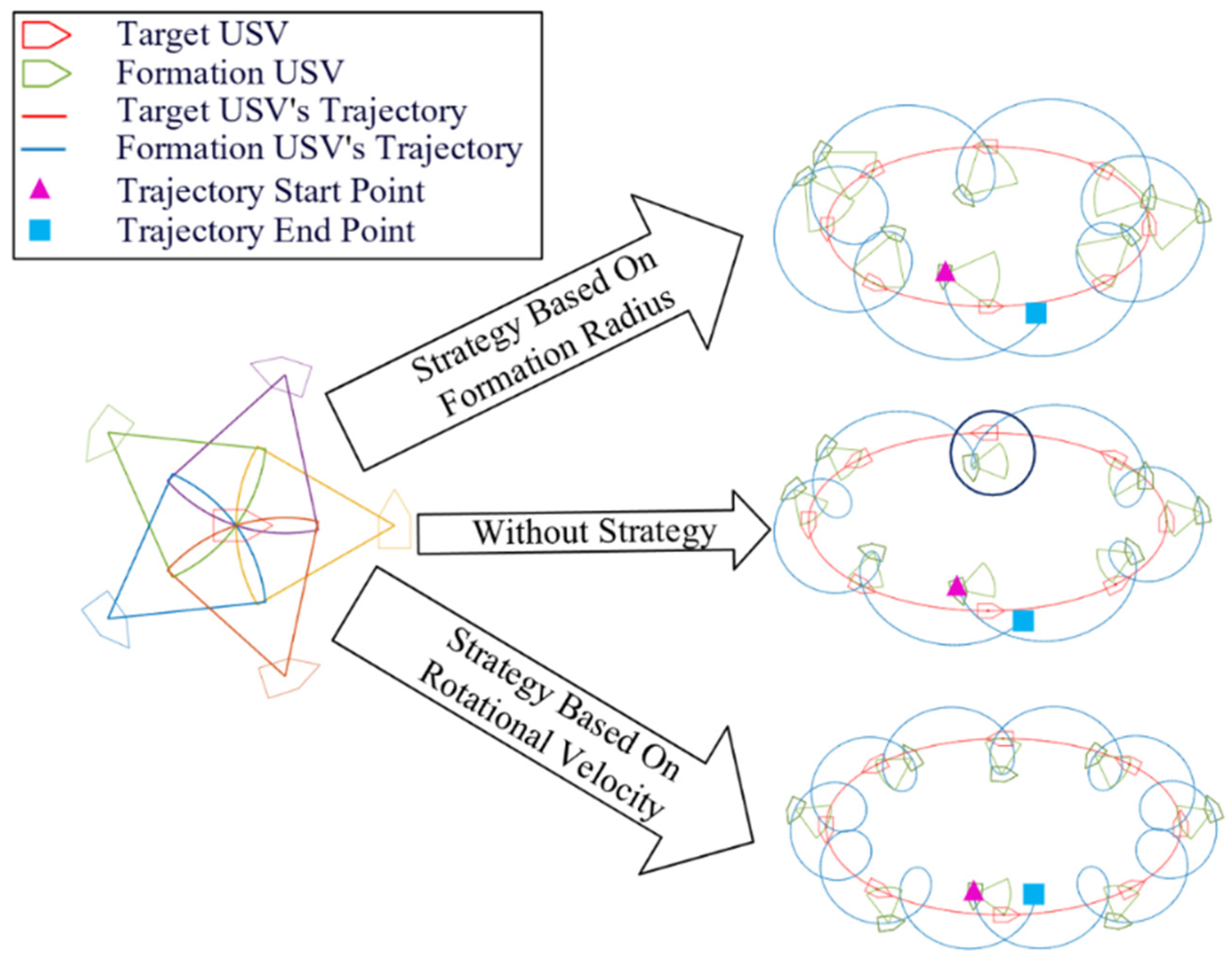
Inspired by [27], we design a circular pattern arrangement of a group of USVs to track and circle the target and employ the virtual structure method to maintain a rigid formation, with the aim to tackle the challenge of performing effective control of the motions of USVs to fully cover the target’s surface and shape throughout the whole processes of tracking, as depicted in Figure 1. A circular formation was adopted to guarantee a structure that facilitates the straightforward observation of the target from multiple angles with a personalized formation radius of each tracking USV equipped with a fixed-direction camera rendering the formation extendable to other shapes when necessary. Target perception stability is ensured as the target remains continuously within the FOV of the surrounding USVs. In addition, our framework allows for the adjustment of the capacity of USVs, improving the system robustness and observation frequency when applied in critical or hazardous environments. Moreover, we innovatively propose a constraint propagation model and four strategies to characterize and analyze the conditions of USV trajectories to simultaneously satisfy both motion and visual constraints in the context of the adoption of the virtual structure method for formation control, based on key parameters of real-time description of the motion state: formation radius and rotational velocity. Furthermore, we examine how target motion and performance affect the selected strategies and the robustness of the strategies.

The remainder of the paper is organized as follows: In Section 2, we introduce the problem description and the model. Section 3 proposes the constraint propagation model and presents four strategies for generating trajectories to surround the target. Section 4 performs comparative analysis and simulation experiments for these strategies. Section 5 examines the effect of target trajectory, sensor noise, and environmental disturbance. Finally, we conclude this paper in Section 6.

2. Problem Description

Consider a moving target USV which is surrounded in the global coordinate system. The position is denoted as ${\left(x_{tar}, y_{tar}\right)}^T\in {\mathbb{R}}^2$, and the heading angle is represented by ${\phi }_{tar}\in \mathbb{R}$. Based on the typical USV kinematic model [28], the motion of the target is given by:

$$\left(\begin{array}{c}{\dot{x}}_{tar}\\ {\dot{y}}_{tar}\\ {\dot{\phi }}_{tar}\end{array}\right)=v_{tar}\left(\begin{array}{c}\cos {\phi }_{tar}\\ \sin {\phi }_{tar}\\ 0\end{array}\right)+{\omega }_{tar}\left(\begin{array}{c}0\\ 0\\ 1\end{array}\right)$$

(1)

where $v_{tar}\in \mathbb{R}$ is the linear velocity and ${\omega }_{tar}\in \mathbb{R}$ is the angular velocity of the target.

Furthermore, the curvature radius of the target is given by:

$$r_{tar}=|v_{tar}/{\omega }_{tar}|$$

(2)

The minimum turning radius is a critical parameter in USV modeling, as the realization of a trajectory must ensure that the curvature radius at any given point exceeds the USV’s minimum turning radius. This requirement is essential for maintaining feasible and safe maneuvers. Moreover, the minimum turning radius of a USV is influenced by both the specific characteristics of the USV model and its operational velocity.

Consider $N$ USVs in ${\mathbb{R}}^2$, denoted with $U=\{u_1,u_2,\dots ,u_N\}$, tasked with tracking a moving target. The positions of the i-th USV are expressed as ${\left(x_i, y_i\right)}^T\in {\mathbb{R}}^2$ and the heading angles are denoted as ${\phi }_i\in \mathbb{R}$, with $i=1, \dots , N$. The kinematic model of the USVs is given by:

$$\left(\begin{array}{c}{\dot{x}}_i\\ {\dot{y}}_i\\ {\dot{\phi }}_i\end{array}\right)=v_i\left(\begin{array}{c}\cos {\phi }_i\\ \sin {\phi }_i\\ 0\end{array}\right)+{\omega }_i\left(\begin{array}{c}0\\ 0\\ 1\end{array}\right)$$

(3)

where $v_i\in \mathbb{R}$ is the linear velocity and ${\omega }_i\in \mathbb{R}$ is the angular velocity of $u_i$.

Consider a polar coordinate system centered at the target, where the direction of the target’s motion is defined as 0°, and counterclockwise is defined as the positive direction. The angle ${\theta }_{ti}$ with a valid range of (−π, π] represents the angle between the center of $u_i$ and the direction of the target’s motion. The rotational velocity of $u_i$, denoted as ${\Omega }_i$, is defined as the rate of change of ${\theta }_{ti}$ over time. Moreover, the distance between $u_i$ and the target is defined as $d_i$. Therefore, the position of $u_i$ in this polar coordinate system is denoted as $\left({\theta }_{ti}, d_i\right)$.

To establish a plane rectangular coordinate system, the 0° direction of the polar coordinate system is designated as the positive x-axis, and the 90° direction is designated as the positive y-axis. The position of $u_i$ in this plane rectangular coordinate system is denoted as:

$$\left(\begin{array}{c}{x}_{ti}\\ y_{ti}\end{array}\right)=d_i\left(\begin{array}{c}\cos {\theta }_{ti}\\ \sin {\theta }_{ti}\end{array}\right)$$

(4)

And the initial time angle information of $u_i$ is given by:

$${\theta }_{ti}(0)=\pi (\left(2i-1\right)/N-1), \mathrm{with} i=1, \dots , N$$

(5)

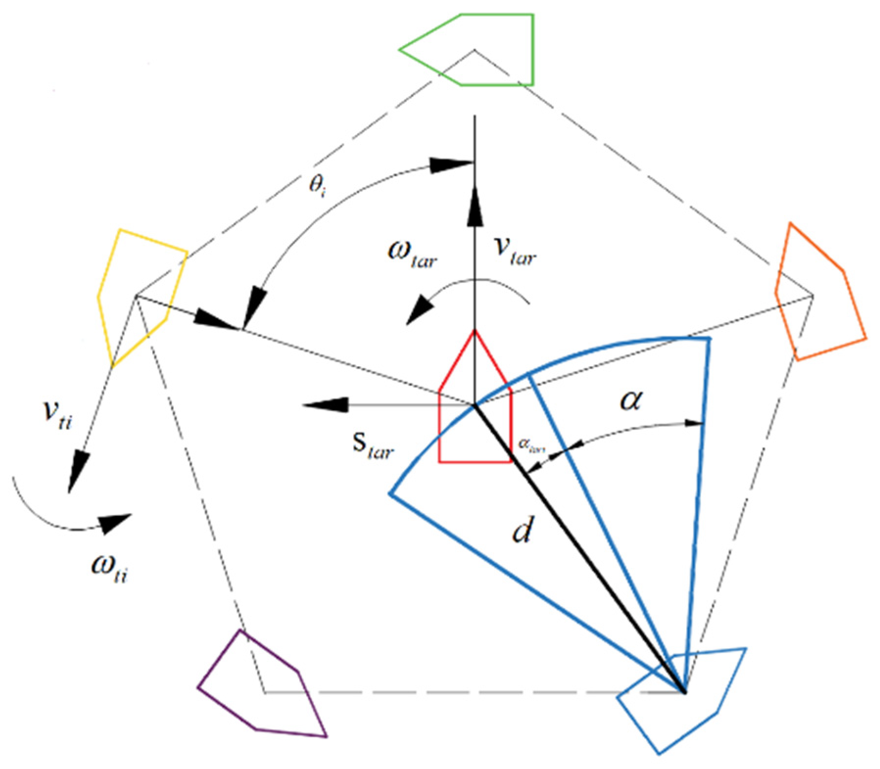
Consider each tracking USV equipped with a fixed camera, rotating counterclockwise around the target in a circular formation. Each onboard camera is positioned to the left, of which the FOV center is directed perpendicular to the bow with a total size of $2\alpha$, as depicted in Figure 2. The angle between the target and the center of the camera’s FOV is defined as ${\mathsf{\alpha }}_{tari}$. Therefore, the condition for the target to remain in the FOV is $\forall {\alpha }_{tari}\in \left[-\alpha , \alpha \right], i=1, \dots , N$.

Within the established framework, the target USV is governed by the USV kinematic model (1), while a group of tracking USVs adopts the USV kinematic model (3). These tracking USVs execute orbital motion to encircle the target. The objective of the problem is to determine control strategies by adjusting either the formation radius (d) or the angular velocity ($\Omega$), ensuring the target consistently remains within the FOV across diverse application scenarios.

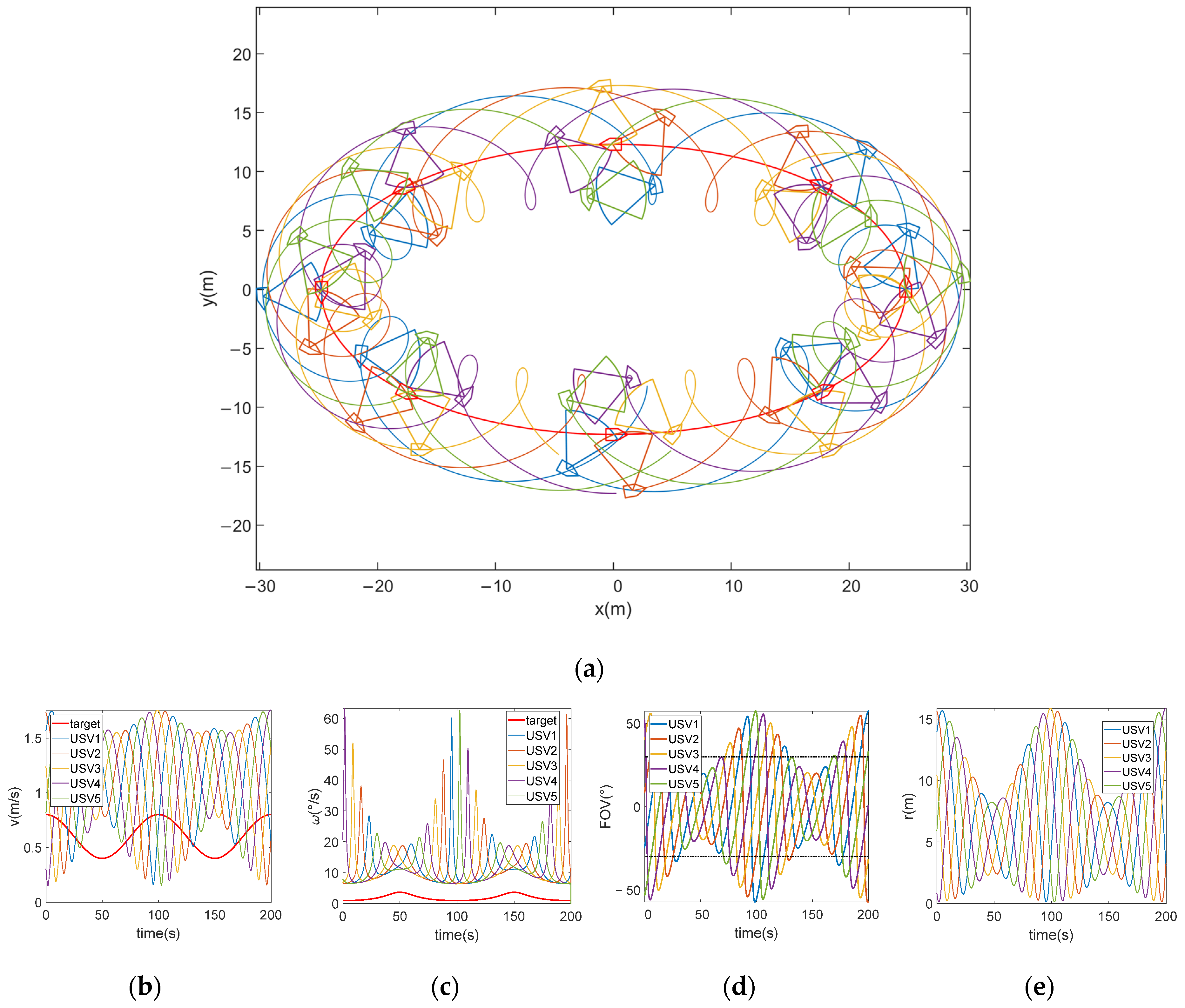
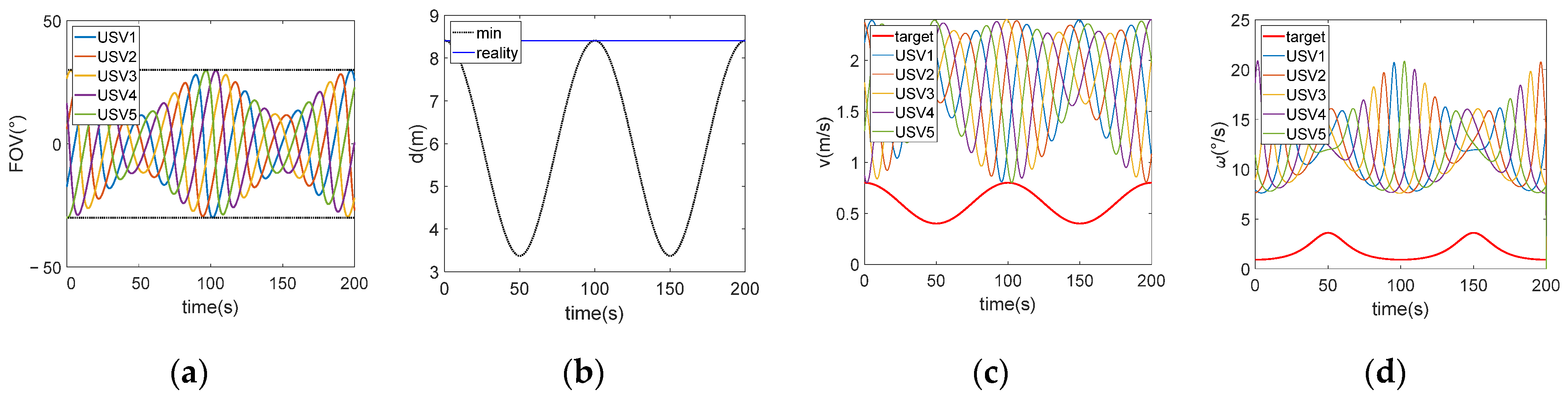
Figure 3 provides an example model that a target follows an elliptical trajectory with a major axis of 25 m and a minor axis of 12.5 m, which remains the same when performing analyses in Section 4, while being circled by five tracking USVs with the formation radius maintained at $d=5 \mathrm{m}$ in an ideal condition while the FOV constraint and kinematic constraint are not included. While circling the target, the tracking USVs perform rotational motion at $\Omega =10°/\mathrm{s}$. Figure 3a shows the trajectory of target and tracking USVs. However, the trajectory of tracking USVs cannot be successfully delivered due to kinematic constraints of tracking USVs based on our analysis. Moreover, the target may temporarily move out of the FOV of certain USVs during phases of steeper motion curves, which is observed in Figure 3d, in which the projection position of the target perceived by the camera of USVs lies beyond their respective FOV at around $t=100 \mathrm{s}$. Figure 3c indicates the violation of FOV constraints is attributed to the relatively high angular velocities of all tracking USVs to maintain the formation at around $t=100 \mathrm{s}$. On the other hand, Figure 3b,c,e suggest an extremely small turning radius, originating from a low linear velocity, and high angular velocity presents difficulty for a tracking USV to take a turn at around $t=100 \mathrm{s}$.

The effect of different formation radii and rotational velocities on the FOV constraints is illustrated as follows.

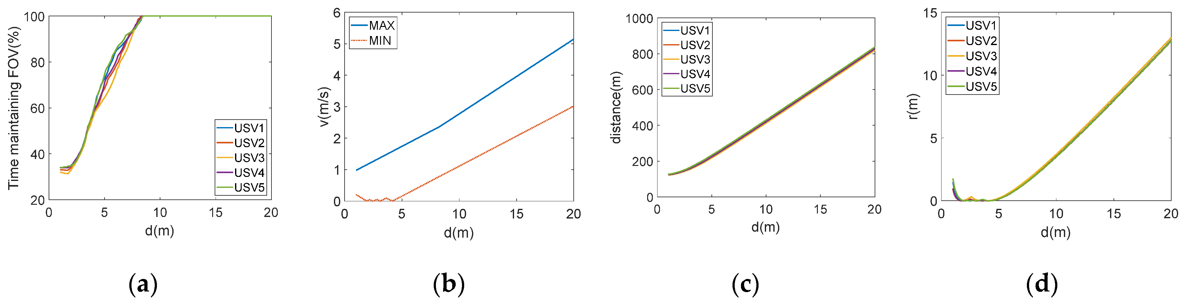
While maintaining the trajectory of the target unchanged, the formation radius of the tracking USVs is varied from 1 to 20 m to study the effect of different formation radii on the target’s visibility in the FOV of tracking USVs. The simulation results are shown in Figure 4. Figure 4a illustrates the percentage of time the target remains within the FOV of each USV in different formation radii over the whole elliptical trajectory. Beyond a certain d of 8.41 m with $\Omega =10°/\mathrm{s}$, the USVs can reliably maintain the target within their FOV. As shown in Figure 4b,c, an increased formation radius leads to a significant rise in the required linear and angular velocities for tracking USVs, placing greater demands on their velocity performance. Additionally, the travel distance also increases substantially. The minimum turning radius of the USVs depicted in Figure 4d varies with the formation radius. At a formation radius of 5 m, the minimum turning radius reaches 0 m and then progressively increases with larger formation radii.

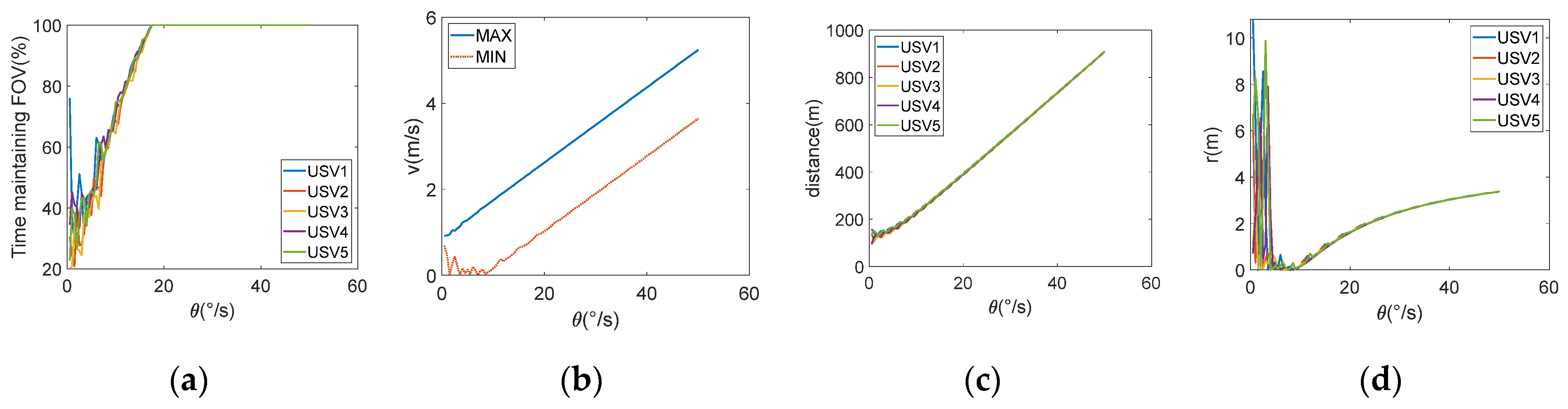
The example in Figure 5 illustrates the effect of different rotational velocities on keeping the target within the camera’s FOV. The simulation from Figure 3 is repeated for various rotational velocities ranging from 0 to 50°/s. Figure 5a indicates that, beyond $\Omega =17.5°/\mathrm{s}$ with $d=5 \mathrm{m}$, the USVs can consistently keep the target within their FOV. Figure 5b,c illustrate that an increase in rotational velocity leads to a significant rise in the necessary linear velocity for the USVs. Additionally, there is a large increase in the distance required to complete a full movement. Figure 5d depicts the minimum turning radius for each USV during this procedure.

3. Constraints on the Reference Trajectory and Strategy Generation

This section presents an introduction to the kinematic constraints and FOV constraints that are crucial to the generation of motion for USVs to effectively circle and track a moving target following a predefined reference trajectory and then proposes the constraint propagation model and strategies of collaborative control.

3.1. Kinematic Constraints

Analyzing the established plane rectangular coordinate system with the target as the origin from the previous section and incorporating the USV kinematic model and the velocity of $u_i$ are performed by:

$$\left(\begin{array}{c}{\dot{x}}_{ti}\\ {\dot{y}}_{ti}\\ {\dot{\phi }}_{ti}\end{array}\right)=v_{ti}\left(\begin{array}{c}\begin{array}{c}\cos {\phi }_{ti}\\ \sin {\phi }_{ti}\end{array}\\ 0\end{array}\right)+{\omega }_{ti}\left(\begin{array}{c}0\\ 0\\ 1\end{array}\right)$$

(6)

where $v_{ti}\in \mathbb{R}$ represents linear velocity and ${\omega }_{ti}\in \mathbb{R}$ represents angular velocity in the plane rectangular coordinate system.

These parameters exist within the local reference frame, and connections are established with the parameters in the global reference frame as follows:

$$\left(\begin{array}{c}{x}_i\\ y_i\end{array}\right)=\left[\begin{array}{cc}\cos {\phi }_{tar}& -\sin {\phi }_{tar}\\ \sin {\phi }_{tar}& \cos {\phi }_{tar}\end{array}\right]\left(\begin{array}{c}{x}_{ti}\\ y_{ti}\end{array}\right)+\left(\begin{array}{c}{x}_{tar}\\ y_{tar}\end{array}\right)$$

(7)

Incorporating Equation (4) into Equation (7), the explicit dependence on $x_{ti}$ and $y_{ti}$ is eliminated, giving the following equation:

$$\begin{array}{ll}\left(\begin{array}{c}{x}_i\\ y_i\end{array}\right)& =d_i\left[\begin{array}{cc}\cos {\phi }_{tar}& -\sin {\phi }_{tar}\\ \sin {\phi }_{tar}& \cos {\phi }_{tar}\end{array}\right]\left(\begin{array}{c}cos{\theta }_{ti}\\ \sin {\theta }_{ti}\end{array}\right)+\left(\begin{array}{c}{x}_{tar}\\ y_{tar}\end{array}\right)\\ & =d_i\left(\begin{array}{c}\cos \left({\theta }_{ti}+{\phi }_{tar}\right)\\ \sin {(\theta }_{ti}+{\phi }_{tar})\end{array}\right)+\left(\begin{array}{c}{x}_{tar}\\ y_{tar}\end{array}\right)\end{array}$$

(8)

Since all tracking USVs in the formation share the same formation radius and angular velocity, the subscripts i in $d_i$ and ${\Omega }_i$ will be omitted in subsequent formulations, denoted simply as d and $\Omega$.

And let ${\theta }_{rel}={\theta }_{ti}+{\phi }_{tar}, {\omega }_{total}=\Omega +{\omega }_{tar}$, calculating the time derivative of Equation (8) to determine the velocities in the x and y directions for $u_i$.

$$\begin{array}{c}{\dot{x}}_i=v_{tar}\cos {\phi }_{tar}+\dot{d}\cos {\theta }_{rel}-d{\omega }_{total}\sin {\theta }_{rel}\\ {\dot{y}}_i=v_{tar}\sin {\phi }_{tar}+\dot{d}\sin {\theta }_{rel}+d{\omega }_{total}\cos {\theta }_{rel}\end{array}$$

(9)

The linear velocity of $u_i$ can be obtained from ${\dot{x}}_i \mathrm{a}\mathrm{n}\mathrm{d} {\dot{y}}_i$ as follows:

$$\begin{array}{ll}{v}_i^2& ={\dot{x}}_i^2+{\dot{y}}_i^2\\ & =v_{tar}^2+{\dot{d}}^2+d^2{\omega }_{total}^2+2v_{tar}\dot{d}\cos {\theta }_{ti}-2v_{tar}d{\omega }_{total}\sin {\theta }_{ti}\end{array}$$

(10)

Given that the USVs perform circular motion around the target, ${\theta }_{ti}$ traverses $(-\mathsf{\pi },\mathsf{\pi }]$ during movement. Consequently, $\cos {\theta }_{ti}$ and $\sin {\theta }_{ti}$ cyclically vary within [−1, 1], enabling the derivation of velocity constraints for $v_i$:

$$v_{i,\mathrm{m}\mathrm{i}\mathrm{n}}^2>{\left(v_{tar}-\dot{d}\right)}^2+d\left(d{\omega }_{total}-2v_{tar}\right){\omega }_{total}$$

(11)

$$v_{i,\mathrm{m}\mathrm{a}\mathrm{x}}^2<{\left(v_{tar}+\dot{d}\right)}^2+d\left(d{\omega }_{total}+2v_{tar}\right){\omega }_{total}$$

(12)

Thus, the performance constraints of the tracking USVs are defined as: $v_{\mathrm{m}\mathrm{i}\mathrm{n}}\le v_{i,\mathrm{m}\mathrm{i}\mathrm{n}} \mathrm{a}\mathrm{n}\mathrm{d} v_{\mathrm{m}\mathrm{a}\mathrm{x}}\ge v_{i,\mathrm{m}\mathrm{a}\mathrm{x}}$.

The heading angle ${\phi }_i$ is computed as:

$${\phi }_i=\mathrm{a}\mathrm{r}\mathrm{c}\mathrm{t}\mathrm{a}\mathrm{n}2\left({\dot{y}}_i,{\dot{x}}_i\right)$$

(13)

where arctan2 is the four-quadrant arctangent function returning values in $(-\mathsf{\pi },\mathsf{\pi }]$, avoiding the quadrant ambiguity of $\mathrm{a}\mathrm{r}\mathrm{c}\mathrm{t}\mathrm{a}\mathrm{n}\left({\dot{y}}_i,{\dot{x}}_i\right)$.

The angular velocity ${\omega }_i$ of $u_i$ is then obtained as follows:

$$\begin{array}{lll}{\omega }_i& =& {\dot{\phi }}_i\\ & =& ({\dot{x}}_i{\ddot{y}}_i-{\ddot{x}}_i{\dot{y}}_i)/({\dot{x}}_i^2+{\dot{y}}_i^2)\\ & =& (v_{tar}^2{\omega }_{tar}+2{\dot{d}}^2{\omega }_{total}+d\dot{d}{\dot{\omega }}_{total}-d\ddot{d}{\omega }_{total}+d^2{\omega }_{total}^3)/v_i^2\\ & & +(\ddot{d}{v}_{tar}-d{v}_{tar}{\omega }_{total}^2-d{v}_{tar}{\omega }_{tar}{\omega }_{total}-\dot{d}{\dot{v}}_{tar})\sin {\theta }_{ti}/v_i^2\\ & & +(2\dot{d}{v}_{tar}{\omega }_{total}+d{v}_{tar}{\dot{\omega }}_{total}+\dot{d}{v}_{tar}{\omega }_{tar}-d{\dot{v}}_{tar}{\omega }_{total})\cos {\theta }_{ti}/v_i^2\end{array}$$

(14)

Given that ${\omega }_i$ comprises thirteen components, many terms can be eliminated during strategy selection. For instance, $\dot{d}$ and $\ddot{d}$ vanish when maintaining a fixed formation radius, thus requiring no specific analysis in this section. Nevertheless, these equations reveal that the formation rotational velocity $\Omega$, as a part of ${\omega }_{total}$ in Equation (14), must coordinate the angular velocities of all tracking USVs to satisfy formation constraints.

3.2. FOV Constraints

In this section, the conditions for generating trajectories that conform to the FOV constraint will be explored. The geometric condition for satisfying the FOV constraint, as determined by the angular relationships depicted in Figure 2, is as follows:

$$\left|\pi /2+{\theta }_{ti}+{\phi }_{tar}-{\phi }_i\right|\le \alpha$$

(15)

Under the premise of satisfying FOV geometric constraints, kinematic constraints are introduced. Based on kinematic Equations (9) and (10), explicit dependency on ${\dot{x}}_{ti}$ and ${\dot{y}}_{ti}$ is removed and then the following equation is obtained:

$$v_{tar}\sin \left({\phi }_{tar}-{\phi }_i\right)+\dot{d}\sin \left({\theta }_{rel}-{\phi }_i\right)+d{\omega }_{total}\cos \left({\theta }_{rel}-{\phi }_i\right)=0$$

(16)

Let FOV angle ${\alpha }_{tari}=\pi /2+{\theta }_{rel}-{\phi }_i$; then, ${\phi }_{tar}-{\phi }_i={\alpha }_{tari}-\pi /2-{\theta }_{ti}$. Using this in Equation (16) and simplifying, the FOV parameterization constraint can be obtained:

$$\tan {\alpha }_{tari}=\left(\dot{d}+v_{tar}\cos {\theta }_{ti}\right)/\left[d{\omega }_{total}-v_{tar}\sin {\theta }_{ti}\right]\le \tan \alpha$$

(17)

Let $D=d{\omega }_{total}-v_{tar}\sin {\theta }_{ti}$. The sign of D is analyzed to simplify (17). Under the fundamental assumption that tracking USVs encircle the target counterclockwise (${\omega }_{total}>0$), $D<0$ implies $d<v_{tar}\sin {\theta }_{ti}/{\omega }_{total}$, which contradicts the physical requirement $d>0.$ Thus, $D>0$ is enforced.

Substituting ${\omega }_{total}=\Omega +{\omega }_{tar}$ into (17) and simplifying, the critical condition emerges:

$$d\left(\Omega +{\omega }_{tar}\right)\ge (\dot{d}\cos \alpha +v_{tar}\cos \left({\theta }_{ti}-\alpha \right))/\sin \alpha$$

(18)

Equation (18) demonstrates that the formation radius d and rotational velocity $\Omega$ must be coordinated to satisfy FOV constraints across all ${\theta }_{ti}$ positions.

The joint satisfaction of kinematic and FOV geometric constraints requires a collaborative mechanism, which will be addressed by the constraint propagation model in Section 3.3.

3.3. Constraint Propagation Model

As discussed in Section 3.2, FOV constraints can be transformed into boundary conditions for formation parameters. This section establishes a constraint propagation mechanism based on these conditions. Unlike traditional single-constraint optimization, the proposed model achieves multi-constraint joint satisfaction through explicit coupling equations, offering a novel paradigm for USV formations.

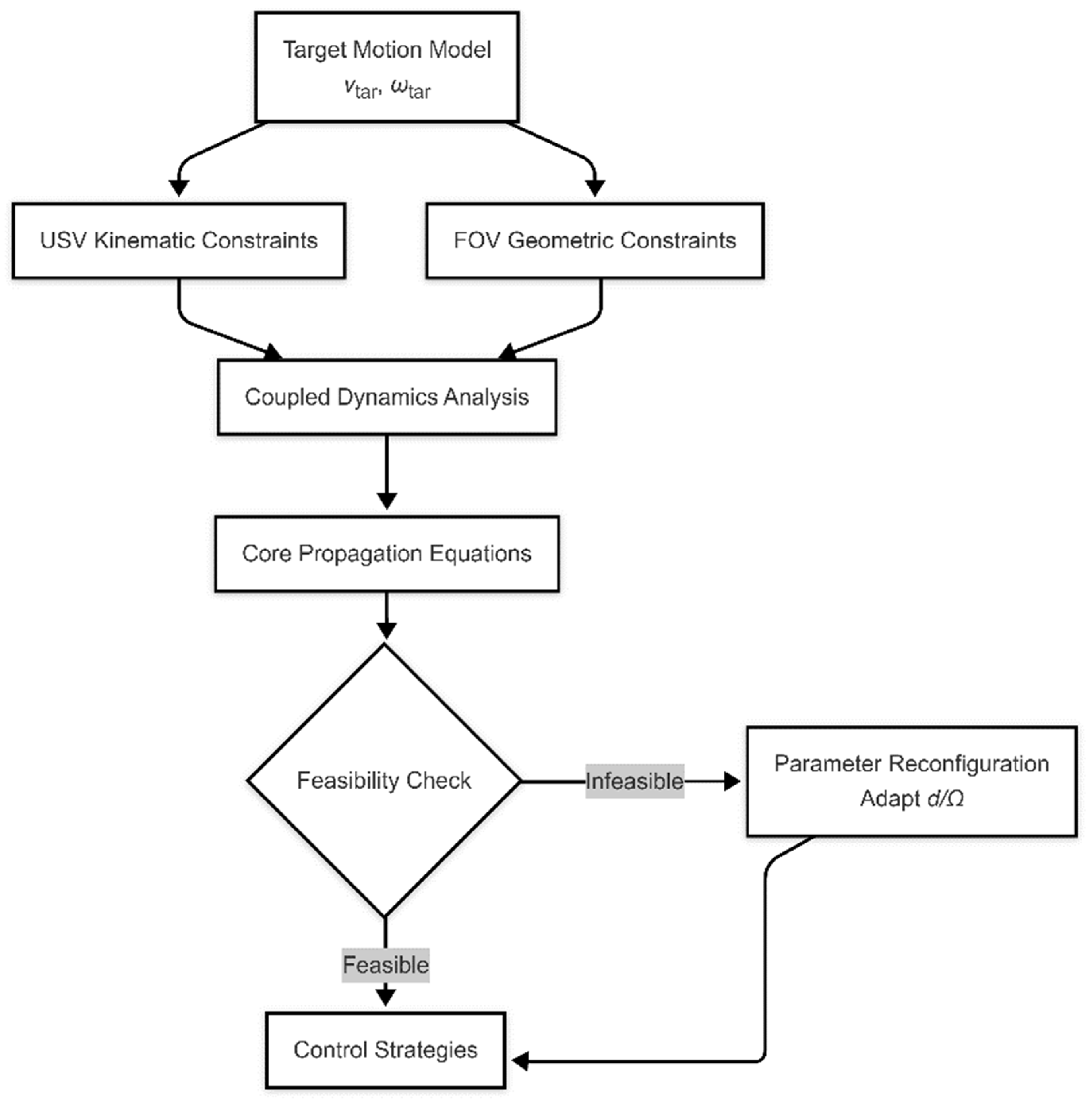
The constraint propagation model coordinates multi-constraint compliance via a three-tier architecture, as illustrated in Figure 6.

As illustrated in Figure 6, the constraint propagation model achieves multi-constraint coordination through a three-tier architecture: the input layer for target motion parameters ($v_{tar}, {\omega }_{tar}$), the fusion layer for kinematic and FOV constraints, and the control strategy generation layer. The model’s core contribution lies in transforming traditionally isolated constraints into a dynamically coupled system, where the interactions between formation radius (d) and rotational velocity ($\Omega$) are explicitly governed by Equation (18).

The model employs hierarchical decoupling design. The formation layer manages global parameters (d, $\Omega$) and the individual layer computes local control inputs ($v_i,{\omega }_i$) based on global parameters.

The feasible parameter space generated by this model directly drives control strategy synthesis in Section 3.4, ensuring rigorous constraint compliance across operational scenarios.

3.4. Collaborative Control Strategy Generation

The following section presents strategies to ensure that the constraints are fulfilled. We assume that the rotational velocity or formation radius changes by a maximum of one quantity. Based on this assumption, two basic strategies are proposed: changing the formation radius $d=d\left(t\right) \mathrm{and} \Omega ={\Omega }_0$ or changing the rotational velocity $\Omega =\Omega (t) \mathrm{and} d=d_0$. Furthermore, two additional strategies are developed: maintaining a fixed formation radius $d=d_c \mathrm{and} \Omega ={\Omega }_0$ or maintaining a fixed rotational velocity $d=d_0 \mathrm{and} \Omega ={\Omega }_c$. Consequently, there are a total of four strategies.

(1)

Fixed formational radius strategy (Fd)

Control parameters: $d=d_c$ and $\Omega ={\Omega }_0$.

It is observed that $\dot{d}=0$ and Equation (18) can be simplified as:

$$d\ge v_{tar}\cos {\theta }_{ti}/\left[\sin \alpha \left({\Omega }_0+{\omega }_{tar}\right)\right]$$

(19)

Therefore, fixed formational radius strategy can be expressed as $d_c=\max \left\{v_{tar}/[\sin \alpha \left({\Omega }_0+{\omega }_{tar}\right)]\right\}$.

(2)

Variable formation radius strategy (Vd)

Control parameters: $d=d(t)$ and $\Omega ={\Omega }_0$.

According to Equation (18), the dynamic adjustment law under this strategy can be expressed as:

$$d(t)\ge \max \left(\left[\dot{d}\cos \alpha +v_{tar}\cos \left({\theta }_{ti}\pm \alpha \right)\right]/\left[\sin \alpha \left({\Omega }_0+{\omega }_{tar}\right)\right]\right)$$

(20)

(3)

Fixed rotational velocity strategy (FΩ)

Control parameters: $d=d_0$ and $\Omega ={\Omega }_c$.

It is observed that $\dot{d}=0$ and Equation (18) can be simplified as:

$$\Omega \ge v_{tar}\cos {\theta }_{ti}/(d_0\sin \alpha )-{\omega }_{tar}$$

(21)

Therefore, fixed rotational velocity strategy can be expressed as ${\Omega }_c=\max \left(v_{tar}/(d_0\sin \alpha )-{\omega }_{tar}\right)$.

(4)

Variable rotational velocity strategy (VΩ)

Control parameters: $d=d_0$ and $\Omega =\Omega (t)$.

According to Equation (18), the dynamic adjustment law under this strategy can be expressed as:

$$\Omega (t)\ge \max \left(v_{tar}\cos ({\theta }_{ti}\pm \alpha )/(d_0\sin \alpha )-{\omega }_{tar}\right)$$

(22)

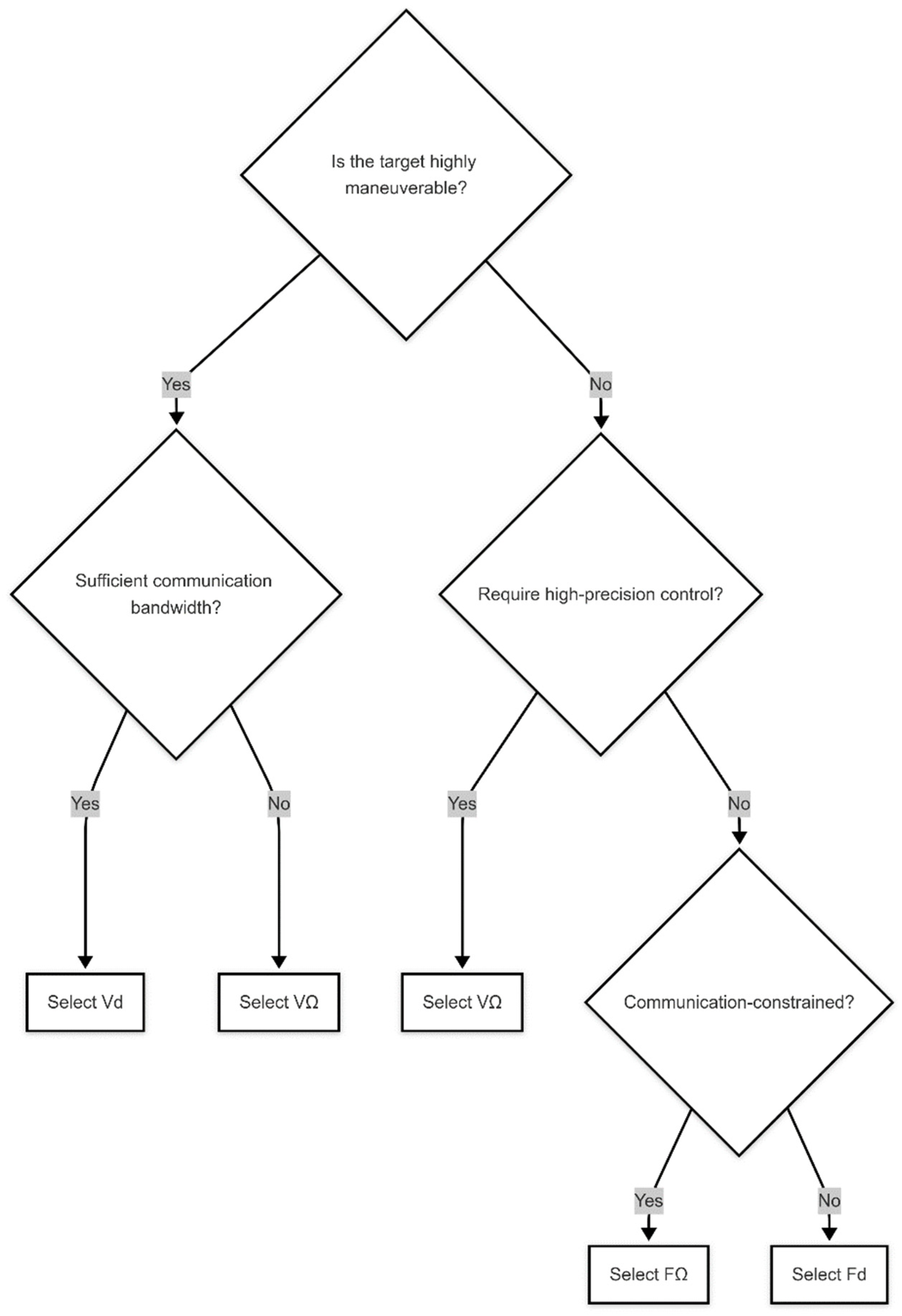
The decision-making workflow employs a three-tiered assessment protocol to optimize strategy selection, as illustrated in Figure 7. First, target maneuverability classification dictates the primary strategy category: highly maneuverable targets activate dynamic parameter adaptation strategies (Vd/V$\Omega$), while steady-motion targets utilize static strategies (Fd/F$\Omega$). Subsequently, communication bandwidth availability is evaluated: sufficient bandwidth enables real-time radius adjustments via the Vd strategy, whereas degraded conditions force reliance on localized velocity optimization (V$\Omega$ strategy) to minimize communication dependencies. Finally, mission-critical precision requirements refine the selection: high-stakes operations mandate V$\Omega$’s trajectory precision, whereas routine monitoring permits simple Fd/F$\Omega$ strategies.

4. Simulation Results

In this section, simulation experiments will be provided to verify the effectiveness of the proposed strategies which can be used to create distinct reference trajectories that comply with the FOV constraints and kinematic constraints simultaneously. In addition, the examination of detailed parameters is presented encompassing travel distance, turning radius, linear velocity, and angular velocity employing different strategies. Moreover, we will discuss the strengths and limitations of the proposed strategies and explore the optimal conditions for their usage.

All simulations were conducted on a single desktop equipped with 32 GB RAM and a 3.60 GHz i7-9700K CPU. The MATLAB R2020a simulation platform was used to establish the simulation environment. It is important to highlight that the simulations were based on the example depicted in Figure 3, wherein the trajectory of the target remains consistent. Furthermore, the individual travel distance can be effectively represented by the mean value, due to the relative consistency across each USV, as illustrated in Figure 4d and Figure 5d.

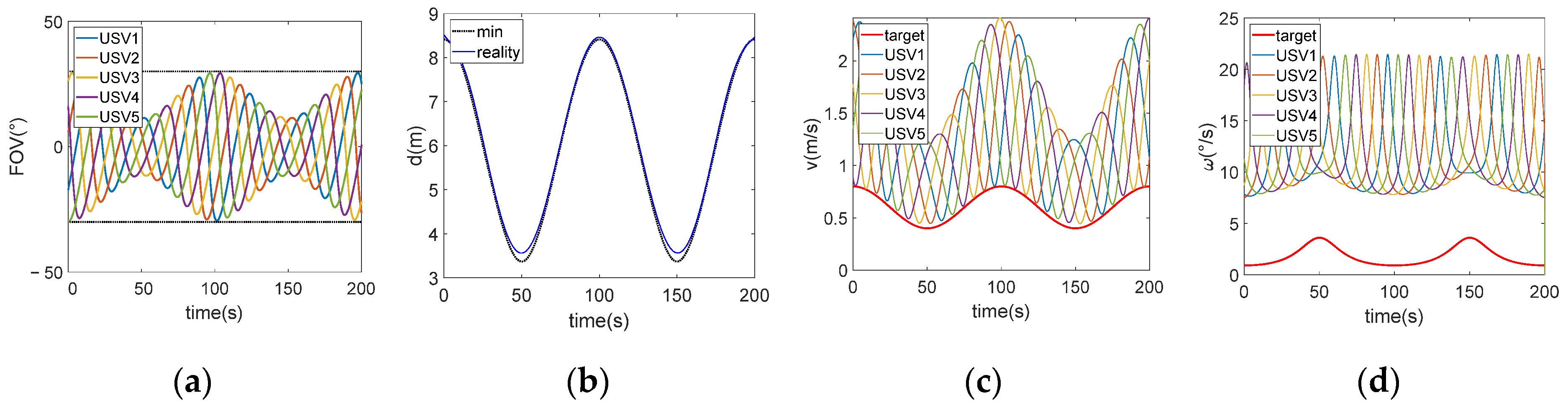
4.1. Fixed Formation Radius Strategy

The formation radius can function as a variable parameter in the formation strategy with FOV constraints, while maintaining a constant rotational velocity for USVs. The strategy of fixed formation radius is defined as determining the formation radius using the extreme values of the FOV limitations derived from the entire target trajectory.

As elaborated in Section 3.4, $d_c=\max \left\{v_{tar}/[\sin \alpha \left({\Omega }_c+{\omega }_{tar}\right)]\right\}$. Substitute the parameters and calculate with the constraint, $d_c=8.41 \mathrm{m}$. The results are illustrated in Figure 8. The overall simulation time of this strategy is 0.274 s.

Figure 8c indicates that tracking USVs exhibit higher average linear velocities when the target possesses a relatively linear velocity, high angular velocity, and, consequently, a small turning radius. Furthermore, Figure 8d shows a narrowed range of angular velocities among the tracking USVs. Additionally, Figure 8a reveals that the target tends to be situated near the central region of the FOV of the tracking USVs. Therefore, it is easier to maintain the target within the FOV when the target motion is intense.

4.2. Variable Formation Radius Strategy

Parameters calculated from Equation (20) are fitted to a curve using the least squares method, focusing on key selected points. The resulting fit is then utilized to adjust the minimum formation radius to meet the FOV constraint. The results of this process are shown in Figure 9. The overall simulation time of this strategy is 0.298 s.

In this scenario, the mean linear velocity of each USV is comparatively low, and the lowest linear velocity aligns with that of the target. The maximum angular velocities for each USV exhibit similarity, and the trend in the minimum angular velocity for tracking USVs corresponds with the angular velocity of the target.

The specific parameters for these two strategies are compared in

Table 1. Parameter Comparison for Two Strategies Based on d.

Parameters	Fixed d	Variable d
Mean Travel Distance (m)	358.078	260.113
Max Linear Velocity (m/s)	2.400	2.410
Peak to Peak Linear Velocity (m/s)	1.543	1.733
Max Angular Velocity (°/s)	20.864	21.486
Mean Period of Velocity (s)	36.1	36.6
Min Turning Radius (m)	2.201	1.196

.

Table 1 indicates that the variable formation radius strategy results in a substantially lower mean travel distance compared to the fixed formation radius strategy, marking the most significant difference between the two approaches. This disparity arises because a smaller radius is adequate to meet the FOV constraints when the target’s angular velocity is relatively high. However, this strategy also reduces the minimum turning radius, requiring the tracking USVs to have stronger maneuverability for the variable formation radius strategy to be effective.

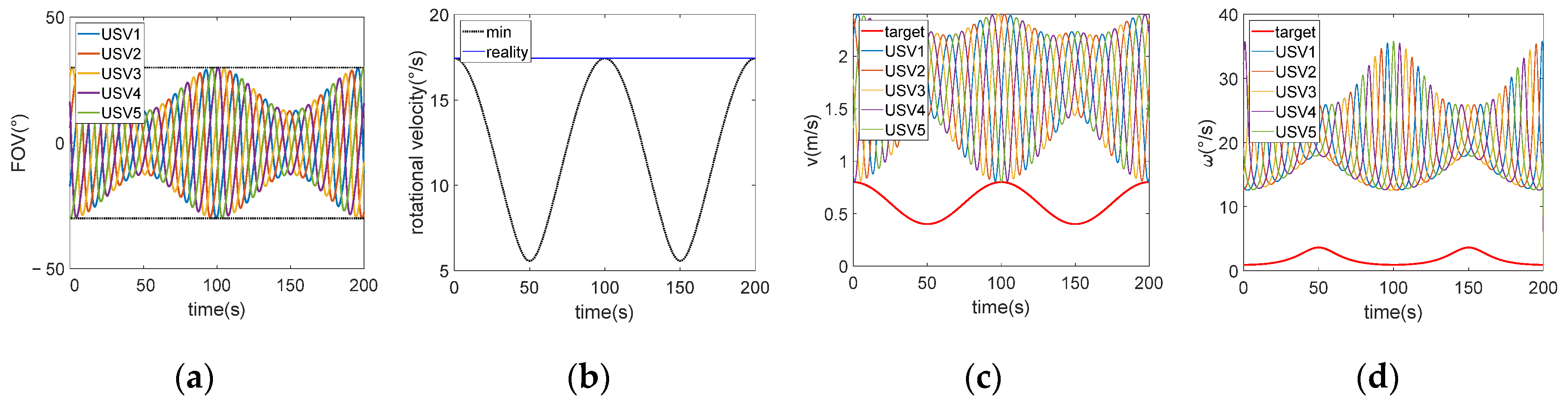
4.3. Fixed Rotational Velocity Strategy

In this strategy, rotational velocity is a variable parameter while formation radius is kept constant. Then, the most straightforward strategy is to define the rotational velocity with the extreme value of the FOV constraint for the full target trajectory.

In this section, the value of ${\Omega }_c$ is determined as $\max \left(v_{tar}/d_c\sin \alpha -{\omega }_{tar}\right)$. Similarly, based on the example presented in Figure 3, substitute the parameters and calculate with the constraint, ${\Omega }_c=17.43°/\mathrm{s}$, and the results are illustrated in Figure 10. The overall simulation time of this strategy is 0.255 s.

When comparing to fixed $d$ or variable $d$ strategies, the period of velocity change is significantly shorter. This is due to the increased rotational velocity, which necessitates more frequent adjustments in velocity to effectively circle the target USV. In this scenario, the maximum linear velocity of the tracking USVs remains mostly constant, while the minimum linear velocity inversely follows the trend of the target’s linear velocity. Regarding angular velocity, the maximum value inversely follows the target’s angular velocity trend, whereas the minimum value aligns with it.

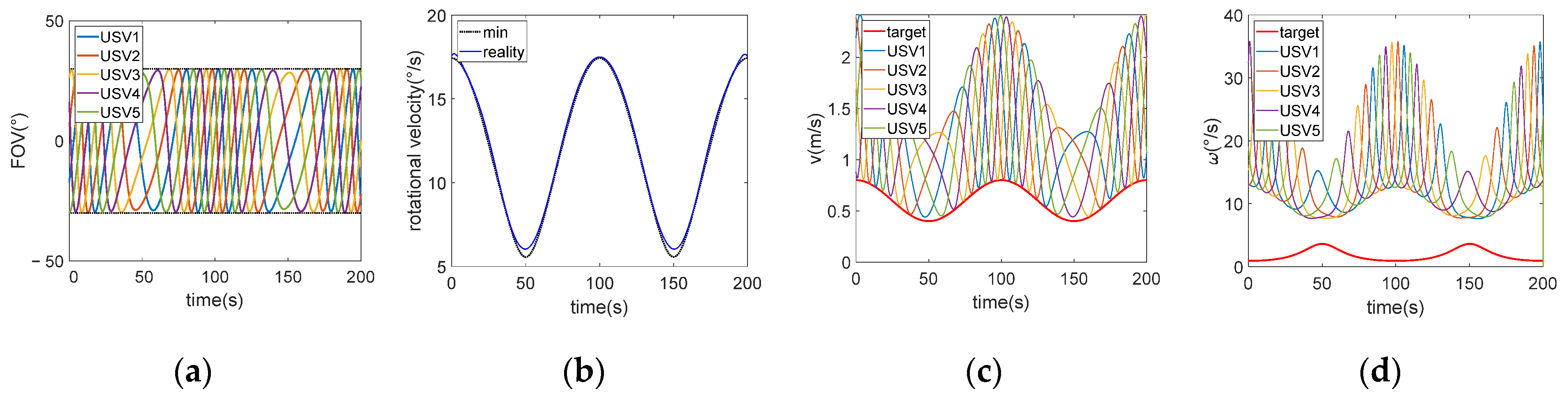
4.4. Variable Rotational Velocity Strategy

Building upon the foundation of Section 4.3, further modifications were introduced. Key points were selected from the maximum values among the minimum values calculated from Equation (22) for $\Omega$, and these points were used for curve fitting via the least square method. The resulting fitted curve was then adjusted using the minimum $\Omega$ value from 4.3 that satisfies the FOV constraints. This process yields the function $\Omega (t)$. Substituting $\Omega (t)$ into the example in Figure 3, the results depicted in Figure 11 were obtained. The overall simulation time of this strategy is 0.332 s.

Based on the data presented in Figure 11, an inverse relationship exists between the angular velocity of the target and the rotational velocity of the tracking USVs. When the angular velocity of the target is high, both the linear and angular velocities of the tracking USVs decrease. Conversely, when the target’s motion is smoother with lower angular velocity, both the angular and linear velocities of the tracking USVs experience a significant increase in response.

The specific parameters for these two strategies are compared in

Table 2. Parameter Comparison for Two Strategies Based on Ω.

Parameters	Fixed Ω	Variable Ω
Mean Travel Distance (m)	347.550	258.749
Max Linear Velocity (m/s)	2.399	2.414
Peak to Peak Linear Velocity (m/s)	1.580	1.679
Max Angular Velocity (°/s)	35.755	35.777
Mean Period of Velocity (s)	20.6	31.1
Min Turning Radius (m)	1.282	1.283

.

The data presented in Table 2 demonstrate a notable similarity in the maximum linear velocity, maximum angular velocity, and minimum turning radius for both strategies. However, the variable $\Omega$ strategy results in a reduced mean travel distance and an increased mean period of velocity change, despite a slight increase in the maximum linear velocity. The variable $\Omega$ strategy has lower requirements for the maneuverability and control of the USVs. However, this strategy has certain limitations, such as the requirement for more complex computations and the fact that the fitting process is strongly influenced by the selection of key data points.

Table 3. Core Characteristics of Proposed Strategies.

Strategy	Fd	Vd	$\mathbf{F}\mathit{\Omega }$	$\mathbf{V}\mathit{\Omega }$
Control Parameters	$d_c,{\Omega }_0$	$d(t),{\Omega }_0$	$d_0,{\Omega }_c$	$d_0,\Omega (t)$
Dynamic Adaptability	Low	High	Moderate	High
Computational Complexity	Low	High	Moderate	High
Control Complexity	Low	Moderate	High	Moderate
Performance Requirements	Low	Moderate	High	High
Energy Consumption	High	Low	High	Low
Key Constraints	Precompute $d_c$ via Equation (19)	Real-time optimization of $d(t)$ via Equation (20)	Precompute ${\Omega }_c$ via Equation (21)	Real-time optimization of $\Omega (t)$ via Equation (22)
Applicable Scenarios	Targets with low angular velocity, long-term monitoring	Highly maneuverable targets, dynamic obstacles	Communication-constrained environments, formation stability prioritized	Complex trajectories, high-precision control
Typical Applications	Long-term marine biology monitoring	Military target tracking	Field missions with limited communication	Urban water search and rescue

compares the core characteristics of four strategies, and their design differences directly map to different scenario requirements.

Comparative analysis in Table 3 elucidates the core characteristics and operational boundaries of four coordination strategies. The fixed formation radius strategy emerges as an optimal solution for steady-state monitoring due to its low complexity, yet its rigid parameter configuration proves inadequate for highly maneuverable targets. The variable formation radius strategy significantly enhances dynamic adaptability through real-time radius optimization, albeit incurring additional computational overhead. The fixed rotational velocity strategy ensures formation stability in communication-constrained environments but it will increase the performance requirements of USVs. Variable rotational velocity achieves high-precision tracking of complex trajectories, demanding high-end hardware support.

5. Effect of Target Trajectory and Robustness of Strategies

5.1. Effect of Target Trajectory

The simulation in Section 4 analyzed strategies under an assumption that the target follows a constant elliptical trajectory with a major axis of 25 m and a minor axis of 12.5 m. In this section, we examine the effects of modifying the motion trajectory of the target on the strategies.

The linear velocity, angular velocity of the target, and the curvature of the trajectory vary over a large range when the target traverses an elliptical trajectory. Various forms of trajectories can be perceived as composite segments that originate from the elliptical trajectory. For example, the linear segments can be organized by connecting the sections of the elliptical trajectory that have a high linear velocity and low angular velocity, and the curved segments can be distinguished based on their curvature and subsequently combined. Therefore, when the target’s trajectory is not elliptical but follows a different path, these strategies can still be effectively applied.

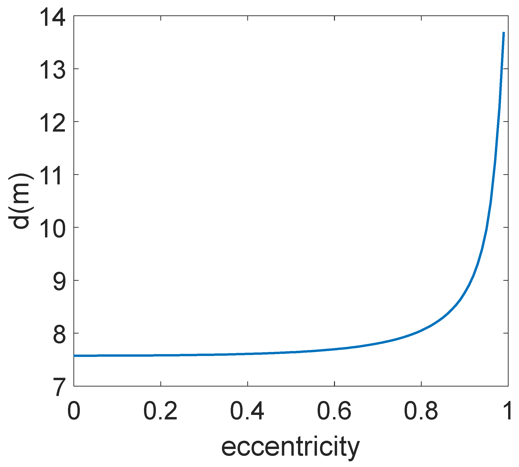
The subsequent part will concentrate on the two strategies that were previously mentioned: maintaining a fixed formation radius and maintaining a fixed rotational velocity, and examine the efficacy of various strategies under different eccentricities in an elliptical trajectory. The range of eccentricity spans from 0 to 1. An eccentricity of 0 indicates a circular trajectory, while an eccentricity of 1 indicates a linear trajectory. The length of the major axis and total travel time of the elliptical trajectory will be held constant throughout the simulation.

In the fixed formation radius strategy, Equation (19) defines that $d_c=\max \left\{v_{tar}/[\sin \alpha \left({\dot{\theta }}_0+{\omega }_{tar}\right)]\right\}$. Given that $\alpha$ and ${\Omega }_0$ are predetermined constants, $d_c$ exhibits a positive correlation with the target’s maximum turning radius. As the eccentricity in the trajectory of the target increases, the minimum turning radius decreases while the maximum turning radius increases. Consequently, the value of $d_c$ also increases, as illustrated in Figure 12.

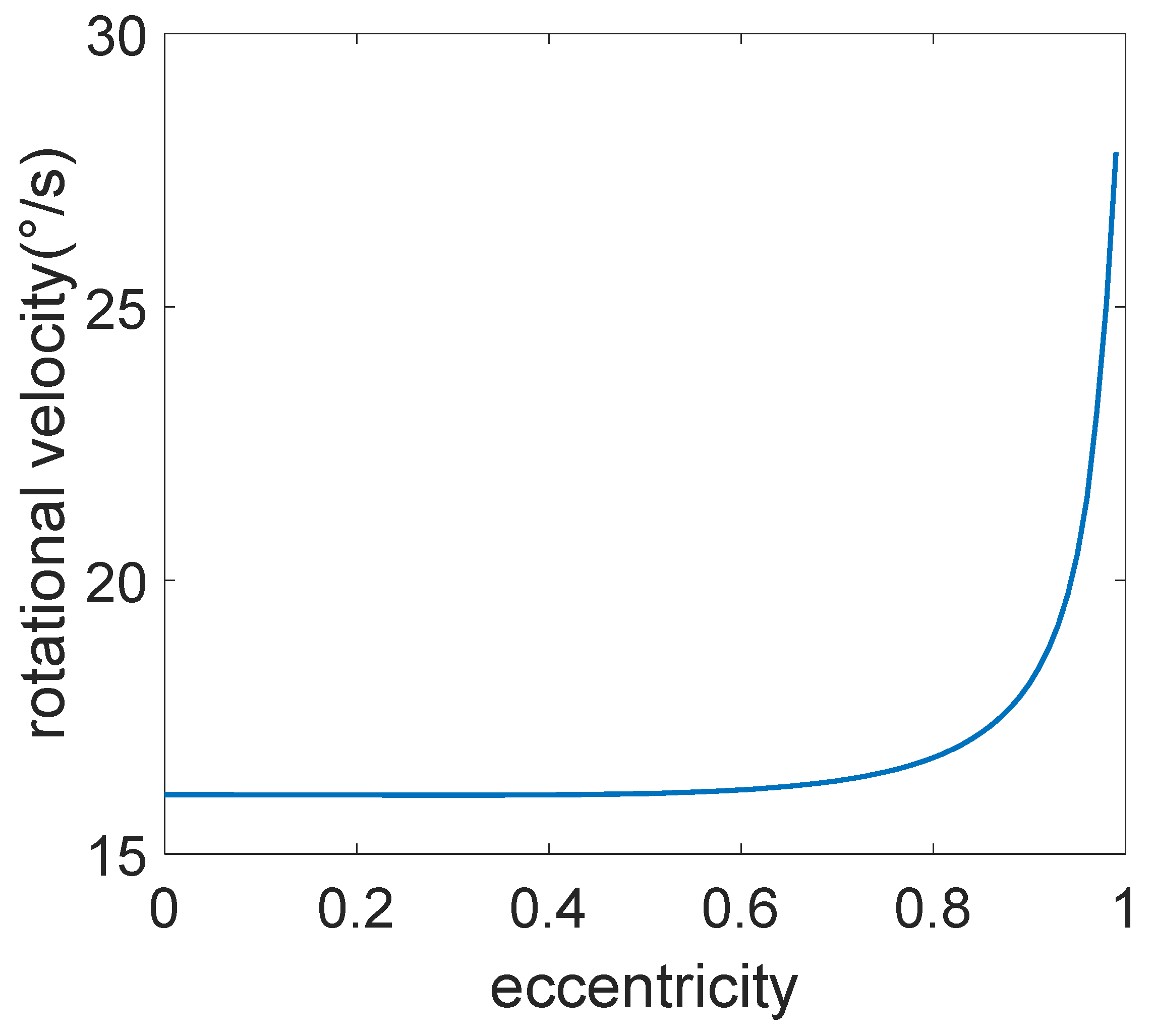
In the fixed rotational velocity strategy, Equation (21) defines that ${\Omega }_c=\max \left[v_{tar}/{(d}_0\sin \alpha )-{\omega }_{tar}\right]$. Given that $\alpha$ and $d_0$ are predetermined constants, considering the signs of the linear and angular velocity terms, it can be concluded that ${\Omega }_c$ is positively correlated with the target’s maximum turning radius. This relationship is illustrated in Figure 13.

5.2. Effect of Sensor Noise

This strategy is still effective in the presence of noise in target velocity perception. We added Gaussian random noise with mean 0 and standard deviation $\sigma$ which varied from 1 × ${10}^{-3}$ to 5 × ${10}^{-3}$ to the velocity of the target used in fixed formation radius and fixed rotational velocity strategies. For each value of $\sigma$, 100 repetitions are performed and the statistical results are represented in

Table 4. Mean and Max Parameters for Strategies under Gaussian Random Noise.

Strategy	Parameter	$\mathit{\sigma } (\times {10}^{-3})$
		1	2	3	4	5
Fixed $d$	mean $d_c$ (m)	8.55	8.71	8.89	9.07	9.27
	max $d_c$ (m)	8.60	8.85	9.15	9.28	9.74
Fixed $\Omega$	mean ${\Omega }_c$ (°/s)	17.64	17.86	18.09	18.32	18.57
	max ${\Omega }_c$ (°/s)	17.69	18.02	18.46	18.59	19.04

.

As demonstrated in Table 4, both fixed formation radius and fixed rotational velocity strategies exhibit inherent noise tolerance through parametric adaptation. For the Fd strategy, increasing $\sigma$ from $1\times {10}^{-3}$ to $5\times {10}^{-3}$ necessitates an 8.4% expansion of mean $d_c$ (from 8.55 m to 9.27 m) and a 13.3% expansion of max $d_c$ (from 8.60 m to 9.74 m), confirming the strategy’s capability to autonomously scale formation geometry based on sensor noise estimates. The F$\Omega$ strategy has a 5.3% expansion of mean ${\Omega }_c$ (from 17.64°/s to 18.57°/s) and a 7.6% expansion of max ${\Omega }_c$ (from 17.69°/s to 19.04°/s), maintaining FOV compliance through angular velocity adjustments that counteract sensor noise. In conclusion, the effectiveness of the strategies can be maintained in the presence of noise by adjusting the formation radius or rotational velocity.

5.3. Effect of Environmental Disturbance

In the marine environment, the impact of wind, waves, and currents on USVs cannot be ignored. In this section, we simulated the process of how wind, waves, and currents affect the tracking of USVs, demonstrating the robustness of the proposed strategy.

To highlight the robustness of the proposed strategy, we assume wind, waves, and currents exert relatively minor disturbances on the target USV but significantly affect tracking USVs. The environmental disturbance settings are specified as follows:

Wind: Modifies the linear and angular velocities of tracking USVs based on wind speed (0–0.2 m/s) and direction (45°).

Wave: Introduces periodic displacement perturbations ($A_{wave}$ = 0–0.2 m, $f_{wave}=0.5 \mathrm{H}\mathrm{z}$) via sinusoidal functions.

Current: Adds a constant velocity drift (0–0.2 m/s, 30°) to displacement increments.

Notably, the velocities above represent environmental impacts on ship motion rather than absolute environmental velocities. Given the maximum target linear velocity of 0.8 m/s in our simulations, environmental disturbances are capped at 0.4 m/s to maintain proportional interference levels. The 0.2 m/s limit ensures environmental disturbances remain below 25% of the target’s max velocity, preventing unrealistic dominance of environmental effects over controlled motion.

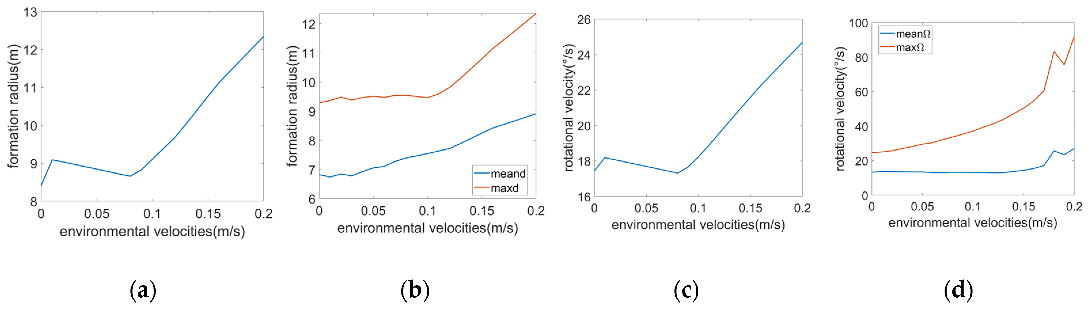
Simulations under these conditions are conducted for all four strategies, with key parameter variations versus disturbance intensity plotted in Figure 14.

As shown in Figure 14, all four strategies necessitate increased d or $\Omega$ values to maintain target visibility within the FOV as wind, wave, and current disturbances intensify. The fixed d strategy exhibits a progressive rise in $d_c$, which increases by 46.7% (reaching 12.34 m) at 0.2 m/s disturbance compared to disturbance-free conditions. Similarly, the variable d strategy shows a 30.6% growth in mean d and 33.0% growth in maximum d. For rotational velocity strategies, the fixed $\Omega$ strategy requires ${\Omega }_c$ = 24.69° (41.7% increase), while the variable $\Omega$ strategy suffers extreme angular velocity demands: maximum $\Omega$ surges by 373% (91.91°/s) and mean $\Omega$ by 204%.

These results demonstrate that augmenting d or $\Omega$ effectively compensates for environmental disturbances to preserve FOV compliance. However, the variable Ω strategy’s precision-dependent nature makes it unsuitable under high disturbances, where its parametric sensitivity exceeds practical hardware limits. In contrast, the fixed d, variable d, and fixed $\Omega$ strategies exhibit superior robustness. This comparative analysis confirms the operational resilience of non-adaptive and semi-adaptive strategies in realistic marine environments.

The analysis in this section indicates that a target exhibiting more intense motion, characterized by a smaller turning radius, enhances the ability to maintain the target within the FOV. Conversely, for targets with a smoother motion and larger turning radii, achieving this objective necessitates either an increased formation radius or a higher rotational velocity. Furthermore, the robustness in sensor noise and environmental disturbance of the strategies has been validated.

6. Conclusions

In the collaborative cooperation of USVs, there is relatively little research that focuses on the exact solutions to circling and tracking a dynamic target. In this paper, we tackled the challenge of keeping a dynamic target within the FOV of tracking USVs while the USVs tracked and circled the target. We proposed a constraint propagation model and four strategies to meet FOV constraints achieved by adjusting the formation radius or the rotational velocity. Strategies based on formation radius ensure a constant observation cycle, while strategies based on rotational velocity maintain a fixed observation distance. Our simulations validated these methods, and we evaluated the effect of the target’s trajectory on two of these strategies. Furthermore, our strategies can guarantee successful target tracking even when there is sensor noise or environmental disturbance.

This research proves beneficial for practical applications such as long-term marine biology monitoring, military target tracking, field missions with limited communication, and urban water search and rescue. The adaptive formation radius or rotational velocity adjustment mechanism contributes to the broader field of distributed multi-agent systems by demonstrating how local sensing constraints can be converted into global formation parameters. This principle could extend to other constrained environments like cave exploration robots where sensor limitations similarly dictate formation geometry.

While this study provides insights into target tracking with FOV constraints, it does not account for wake effects generated by the target. In practical applications, wake propagation may interact with tracking USVs, potentially leading to vortex-induced vibrations. Future work will extend the present model to incorporate wake dynamics and evaluate its impact under realistic multi-physics scenarios.