Abstract
Ship type (e.g., Cargo, Tanker and Fishing) classification is crucial for marine management, environmental protection, and maritime safety, as it enhances navigation safety and aids regulatory agencies in combating illegal activities. Traditional ship type classification methods with AIS data are often plagued by problems such as data imbalance, insufficient feature extraction, reliance on single-model approaches, or unscientific model combination methods, which reduce the accuracy of classification. In this paper, we propose an ensemble classification method based on a stacking strategy to overcome these challenges. We apply the SMOTE technique to balance the dataset by generating minority class samples. Then, a more comprehensive ship behavior model is developed by combining static and dynamic features. A stacking strategy is adopted for the classification, integrating multiple tree structure-based classifiers to improve classification performance. The experimental results show that the ensemble classification method based on the stacking strategy outperforms traditional classifiers such as CatBoost, Random Forest, Decision Tree, LightGBM, and the ensemble classification method, especially in terms of improving classification precision, recall, F1 score, ROC curve, and AUC. This method improves the accuracy of ship type recognition, and it is suitable to real-time online classification, which is helpful for applications in marine safety monitoring, law enforcement, and illegal fishing detection.
1. Introduction
The Automatic Identification System (AIS), developed by the International Maritime Organization (IMO), is a standardized digital navigation system that enables automatic ship tracking and real-time data exchange between nearby ships, AIS shore stations, satellites, and other devices. By broadcasting dynamic navigation parameters and static vessel attributes, AIS provides essential information for maritime safety and regulatory compliance. With the improvement of AIS availability, AIS applications have extended from early navigation to various fields [1], such as ship type classification [2,3], abnormal ship behavior detection [4,5,6], ship trajectory recognition [7,8,9], maritime supervision [10,11,12], and navigational risk assessment [13,14].
These studies based on AIS data usually have high data quality requirements, which are not readily available in real applications. For example, researchers and vessel traffic service (VTS) operators were dissatisfied with 74 percent of the ship types observed [15]. Different types of ships have different berth, anchoring (mooring) spacing, and dimensional compatibility, as well as differences in ship maneuverability, acceleration, heading stability, and turning performance. Incorrect ship type identification will not only affect water traffic management and marine safety but also AIS data applications. It is worth noting that some ships engaged in illegal activities may evade detection by sending fake information, such as ship type [16]. The accurate identification of ship types in AIS data is crucial for combating illegal activities, especially in the regulation of illegal fishing and overfishing. Accurately ship type classification can effectively monitor suspicious activities and provide data support to combat illegal fishing behavior. In addition, precise ship classification is of great significance for improving maritime traffic safety and efficiency, strengthening marine environmental protection, optimizing port and logistics management [17], and ensuring national defense and border security [18].
Contemporary ship type classification research follows three methodological paradigms based on data modality. One is based on image data, such as synthetic aperture radar (SAR) and optical satellite images, which mainly use Convolutional Neural Networks (CNNs) to recognize the basic features of ship images and gradually focus on fine-grained ship type classification [19,20,21,22,23,24,25]. The other is directly based on AIS dynamic and static data [2,3,15,26,27,28], and the third is a combination of the two [29,30].
Compared with the first and third methods introduced above, directly extracting geometric and motion behavior features from AIS data is simpler, faster, and more efficient. The required data are easier to obtain and can fully utilize the spatiotemporal information of AIS data. It is more suitable for real-time maritime navigation safety monitoring systems, and many scholars have conducted relevant research and made certain progress. In Refs. [31,32,33], researchers divided fishing boats into trawl fishing, purse seine fishing, longline fishing, etc. However, they were based on the different behavioral patterns of fishing boats, which were only suitable for special scenarios. In order to classify and study more types of ships, Duan et al. [2] developed a semi-supervised framework employing variational autoencoders (VAEs) for multi-class vessel classification (Fishing/Passenger/Cargo/Tanker), synergistically integrating discriminative and generative learning to effectively utilize both labeled and unlabeled data, thereby addressing label scarcity challenges in supervised maritime classification. Yan et al. [3] fully considered the dynamic and static information of ships, and 13 dimensional features including geometric and behavioral features were formed. Two classifiers, XGBOOST and RF, were applied to classify ships into Cargo, Tanker, Fishing, Passenger, and Tug. Huang et al. [26] used eight classification algorithms based on tree structure, proximity, and regression to classify Bulk Carriers, Containers, General Cargo, and Vehicle Carriers. The results show that tree structure-based algorithms, especially XGBOOST and Random Forest, exhibit superior performance. They have made some progress in various types of ship classification, but they have not considered the impact of data imbalance on ship classification. In fact, there are significant differences in the number of different types of ships in most research areas, which leads to a bias towards the majority class in model predictions and a decrease in the classification performance of minority classes [34]. In addition, imbalanced samples can lead to the model overly focusing on majority class samples and ignoring minority class samples during training, resulting in overfitting. Due to the model’s excessive focus on the majority of class samples, its generalization ability to new data decreases. Even though the accuracy of the model is high, its predictive performance may not be ideal in practical applications, especially for predicting minority class samples. Amigo et al. [27] presented an analysis over eleven trajectory segmentation techniques applied to the study and experimentation of ship classification problems based only on kinematic information, without fully utilizing the static data of AIS. In fact, different types of ships have different lengths, widths, draft depths, etc., which helps to improve the accuracy of ship classification. Furthermore, this may result in the limited performance of the model in practical applications.
Unlike previous research that predominantly focused on individual machine learning algorithms or their incremental modifications, recent advances in ensemble learning have demonstrated superior performance across classification tasks, ship trajectory extraction, and regression problems, achieving enhanced accuracy, accelerated training efficiency, and improved generalization capabilities [35,36,37,38]. Some scholars tried to use ensemble learning algorithms to conduct research on ship type classification. Wang et al. [39] proposed an integrated classification method MFELCM (Multi-Feature Ensemble Learning Classification Model), and proved that MFELCM is better than the base classifiers. In the latest study, Meyer et al. [40] used the ensemble machine learning algorithm LightGBM to classify ships into Cargo, Fishing, Passenger, Port, Recreational, and Tanker, and he studied the impact of different feature combinations on the classification results, which achieved similar results compared with MFELCM. They used ensemble learning methods to improve the accuracy of ship classification, but only simply combined the base models without fully analyzing their advantages to obtain better classification results.
To address the challenges in ship type classification with AIS data, this study proposes an ensemble classification method based on a stacking strategy, achieving an overall precision of 91%, recall of 88.7%, F1-score of 89.5%, and AUC of 96.7% on imbalanced datasets.
2. Methodology
This study proposes an ensemble classification method based on a stacking strategy, aiming to improve the accuracy and robustness of ship type classification. The flow diagram of this method is shown in Figure 1, which mainly consists of the following steps.
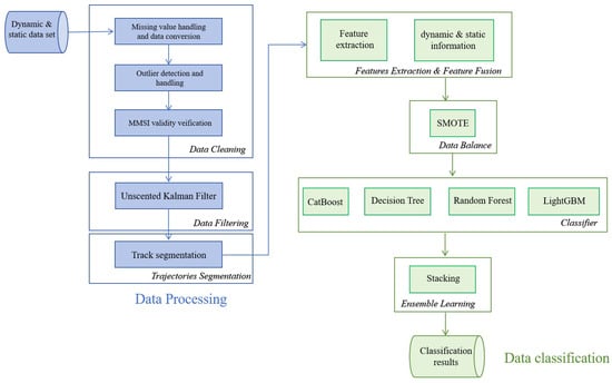
Figure 1.
Flow diagram.
2.1. Data Selection
Through researching the literature, common dynamic indicators in such studies include the Speed Over Ground (SOG), Course Over Ground (COG), heading, longitude, and latitude. These indicators can reflect the real-time navigation status and movement mode of the ships. Maritime vessels exhibit distinct design specifications and kinematic signatures correlated with their functional roles. Cargo and Tanker ships demonstrate notably different motion patterns compared to Fishing ships, particularly in acceleration/deceleration latency (attributable to greater mass inertia) and navigational trajectories. These operational disparities are systematically encoded in dynamic data through vessel-specific docking port positions and route optimization behaviors.
At the same time, some researchers have begun to explore the potential impact of incorporating static indicators on analysis [2,3]. There are significant differences in size among different types of ships. For example, the average length and width of Cargo are much larger than Fishing ships, and we can enhance the ability to distinguish ship types through static indicators.
The joint use of these two types of data brings multiple benefits, as follows:
- Rich information dimensions: Combining static and dynamic features can provide a panoramic view, allowing us to comprehensively grasp the behavior of ships. For example, different ship types can affect their turning radius due to their design, and the speed of the ship is often constrained by its length and displacement.
- Enhance analytical ability: By simultaneously considering the identification information and behavior patterns of the ships, it is possible to more accurately distinguish the motion rules of different types of ships.
- Improving model performance: In machine learning prediction or classification tasks, the application of multidimensional features often leads to higher accuracy because they provide more information about the target variable. Therefore, we combined static and dynamic data for comprehensive analysis.
Static data include the fixed attributes of ships. Considering the analysis objectives, we have selected the following four features: MMSI (Maritime Mobile Service Identity), ship type, ship length, and ship width. MMSI is the unique identifier for each ship, which can be used to track the activity records of individual ships and merge them with the dynamic data in the following text. The physical dimensions of a ship, such as its length and width, as well as its type, are key factors that affect its motion characteristics. Ship type is the target variable, which is used to train the models in the training phase and verify the accuracy of the models collected with external data in the testing phase.
Dynamic data contain information about ship motion and are an essential part of predictive models. In this study, we focus our attention on the following dynamic features: longitude, latitude, SOG, COG, and heading. These data not only reflect the real-time navigation status of the ship, but also reveal its movement patterns.
2.2. Data Preprocessing
In order to ensure the quality of the dynamic data used and its positive impact on the model, we carried out a series of preprocessing steps, including data cleaning, denoising, and trajectory division.
In this study, static records include key vessel attributes such as MMSI, ship type, length, and width, providing information about the ship’s identity and dimensions (Table 1). On the other hand, dynamic records contain motion-related data such as longitude, latitude, speed, and heading, which reflect the real-time navigation status and movement patterns of the vessel (Table 2).

Table 1.
Static Data.
Table 2.
Dynamic Data.
2.2.1. Data Cleaning
- Missing value handling and data conversion: We adopt a deletion strategy for missing values in static and dynamic data to ensure data integrity. Convert some character types to numerical types, such as converting the length and ship width from character types to numerical types, and delete records that cannot be converted.
- Outlier detection and handling: Outliers may be caused by data entry errors or measurement errors. We checked for parameters including the ship length, ship width, speed, course, heading, latitude, and longitude, and we removed records that were clearly not in line with reality, such as data points where the ship length and width were 0 or the speed, course, and heading exceeded the normal range [26,41].
- MMSI validity verification: According to the requirements of the International Maritime Organization, all MMSI records are expressed as a 9-digit code and clean up illegal MMSI records [42].
2.2.2. Noise Reduction Processing
Based on the characteristics of AIS data, noise reduction processing is crucial. AIS datasets are inherently susceptible to noise artifacts caused by signal interference, equipment malfunctions, and human factors such as manual input errors or delayed/missing data transmissions. Unprocessed noise can critically compromise downstream analytical tasks, including trajectory reconstruction and behavioral pattern identification. The trajectory before noise reduction is usually scattered and incoherent. For example, some scattered points that deviate from the main route may be noise points. After noise reduction processing, the trajectory becomes smoother and more coherent, providing a high-quality foundation for further data analysis.
Currently, noise filtering methods include heuristic filtering, median filtering, and Kalman filtering [43]. Compared to traditional Kalman filters and extended Kalman filters, the Unscented Kalman Filter (UKF) [44] effectively handles nonlinear ship motion patterns, reducing noise while preserving trajectory continuity [45]. It is a key algorithm used in dynamic data preprocessing to smooth data and reduce noise caused by sensor errors, signal loss, or environmental factors.
The Unscented Kalman Filter adopts the Unscented Transform (UT), which approximates the probability distribution by selecting a set of sample points (called Sigma point set). These points can accurately capture the mean and covariance of the original probability distribution, and when they pass through a nonlinear function, a good estimate of the output distribution can be obtained [46].
- Initialization: Set the initial state estimation vector UKF x and the initial state covariance matrix UKF P. Define the covariance matrices for process noise and observation noise, denoted as UKF Q and UKF R.
- Select the Sigma point: Generate a set of Sigma points to capture the mean and covariance information of the state vector.
- Prediction steps: Pass the Sigma point through the state transition function fx to predict the state distribution at the next moment. Calculate the predicted state mean and covariance based on the predicted Sigma points.
- Update steps: Pass the predicted Sigma points through the observation function hx to estimate the observed values.When obtaining new actual observation data, calculate the Kalman gain by combining the predicted observation Sigma points.Update state estimation and state covariance using Kalman gain.
- Handling outliers: During the prediction and update process, attention should be paid to detecting and removing outliers that exceed the reasonable range of navigation parameters, such as unexpected high-speed movements or impossible course changes.
- Repeat the prediction update cycle: Repeat the prediction and update steps for each new observation in the data stream.
The advantage of the Unscented Kalman Filter lies in its powerful modeling ability for nonlinear systems, making it widely used in various engineering and scientific fields. After applying the UKF, we obtained smoother and less noisy data, providing cleaner and more reliable datasets for subsequent model training.
2.2.3. Trajectory Division
Based on the communication frequency of the AIS and actual navigation behavior, trajectory division is carried out to ensure that each trajectory segment has spatiotemporal coherence and information integrity. The communication frequency of the AIS is at least once every 10 s. Based on this, the interval for effective trajectory measurement should not exceed 11 s [47]. To better capture the typical motion patterns of the ship, such as steering and speed changes, we ensure that each trajectory segment contains at least 50 data points. So we select 50 data points as the criteria for segmenting trajectories [48]. This can avoid introducing too much noise while maintaining data coherence.
By following these steps, we can effectively refine the dataset and provide high-quality input for feature engineering and machine learning model training, ensuring that the research outcomes accurately capture the complexity of ship type classification.
2.3. Dynamic Feature Extraction
Dynamic feature extraction focuses on obtaining attributes that change over time from the ship’s motion trajectory.
- 1.
- Average speed (avg_speed)Definition: The arithmetic mean of the sailing speeds of all trajectory points.Calculation method: The speed for each trajectory point is directly given by the AIS data. The average speed is then calculated by averaging these individual speeds over the observation period.Purpose: It reflects the general operating speed level of the ship, which helps to understand the normal operating speed of the ship.
- 2.
- Maximum speed (max_speed)Definition: The highest observed speed value in all records.Calculation method: Select the maximum value from all calculated speed values.Purpose: It reflects the maximum speed of the ship, which helps to understand the dynamic performance of the ship.
- 3.
- Minimum speed (min_speed)Definition: The lowest observed speed value among all records.Calculation method: Select the minimum value from all calculated speed values.Purpose: May be related to ship stopping, waiting, or very slow movement.
- 4.
- Standard deviation of sailing speed (std_speed)Definition: The standard deviation of the speed value, which measures the degree of speed fluctuation.Calculation method: Calculate the deviation of all speed values relative to the average speed, and then obtain the standard deviation.Purpose: It reflects the stability of the ship’s speed, and large fluctuations may indicate changes in sea conditions or other interference factors encountered during navigation.
- 5.
- Average course (avg_course)Definition: The arithmetic mean of the course of all trajectory points.Calculation method: Calculate the arithmetic mean of the course (e.g., angle value) of all trajectory points.Purpose: It displays the main navigation direction of the ship and can be used to determine whether the ship is following the established route.
- 6.
- Standard deviation of course (std_course)Definition: The standard deviation of the course value, which measures the degree of course fluctuation.Calculation method: Calculate the deviation of all course values relative to the average course and then obtain the standard deviation.Purpose: Indicates the frequency and degree of changes in the ship’s course, with larger values indicating that the ship may have experienced complex sailing environments or frequent adjustments to its course.
- 7.
- Average heading (avg_heading)Definition: The arithmetic mean of the heading of all trajectory points.Calculation method: Calculate the arithmetic mean of the heading of all trajectory points.Purpose: It displays the main projection direction of the longitudinal axis of the ship in the horizontal plane and can be used to describe the direction of a ship’s movement.
- 8.
- Standard deviation of heading (std_heading)Definition: The standard deviation of heading value, which measures the degree of heading fluctuation.Calculation method: Calculate the deviation of all heading values relative to the average heading and then obtain the standard deviation.Purpose: Indicates the frequency and degree of changes in the ship’s heading.
- 9.
- Center longitude and center latitude (center_lon and center_lat)Definition: The geographic center point of longitude and latitude values for all trajectory points.Calculation method: Calculate the arithmetic mean of the longitude and latitude values of all trajectory points separately.Purpose: Represents the geographic center position of the trajectory coverage area, helping determine the main activity area of the ship.
2.4. Feature Fusion
Feature fusion is a critical step in data preprocessing, which involves the combination of features from different sources and types into a comprehensive dataset for more thorough analysis and modeling.
We merge the dynamic feature set calculated in the previous step with the static features and then clean the merged data to ensure the removal of any missing or outlier values, thereby forming a complete and clean feature set. This feature set encompasses both the physical attributes of the ship and its behavioral characteristics, providing the necessary input data for subsequent machine learning models.
Dynamic data include dynamic features such as ‘MMSI’, ‘avg_speed’, ‘max_speed’, ‘min_speed’, ‘std_speed’, ‘avg_course’, ‘std_course’, ‘avg_heading’, ‘std_heading’, ‘center_lon’, and ‘center_lat’. Static data include static features such as ‘MMSI’, ‘length’, and ‘width’. The mathematical expression of feature fusion can be imagined as a joint operation of two sets as follows:
2.5. Handling Data Imbalance Issues
In machine learning classification tasks, the uneven distribution of categories in the dataset is a common and challenging problem. When the sample size of certain classes in the dataset is significantly larger than other classes, the model tends to predict the majority class, resulting in weaker recognition ability for minority classes. This bias has a significant impact on model performance, especially in multi classification scenarios. For example, in ship type classification tasks, if the number of ships in one type is much larger than other types, the model may favor that type and ignore classes with fewer numbers.
To address this challenge, SMOTE (Synthetic Minority Over Sampling Technique) [49] technology was introduced in the data preprocessing stage, aiming to balance the class distribution by synthesizing new minority class samples. The core idea of the SMOTE algorithm is not simply to replicate existing minority class samples but to generate new synthetic samples to increase the representativeness of minority classes. The working principle of this algorithm is as follows:
- For each sample in the minority category, the algorithm finds its k-nearest neighbor sample.
- The algorithm randomly selects a point between the selected neighbor sample and the original sample, and it performs linear interpolation between these two samples to generate a new sample.
- This process will be repeated for all samples in the minority class until the sample size of the minority class is close to or equal to that of the majority class.
SMOTE technology can help improve the model’s ability to recognize minority classes, providing an effective strategy for solving data imbalance in ship type classification and further enhancing the overall prediction accuracy and robustness of the model.
2.6. Ship Type Classification
In addressing the challenges of ship type classification, we develop an ensemble classification method based on a stacking strategy to mitigate the inherent limitations of single-model approaches. Single-model architectures exhibit inherent limitations in anti-interference capability when processing noisy maritime data streams. Therefore, we hope to integrate multiple models and combine their advantages and disadvantages to improve the model’s generalization ability. Ensemble learning methodologies primarily operate through three paradigms. Boosting employs sequential weak learner training, where each subsequent model prioritizes misclassified instances from predecessors to incrementally reduce residual errors. Bagging utilizes parallel independent learners trained on bootstrap-sampled data subsets, aggregating predictions through majority voting or averaging to mitigate overfitting. Stacking implements a hybrid architecture with base learners generating preliminary predictions from raw inputs, which are then vertically concatenated as meta-features for a secondary model (meta-learner) to produce final outputs. This hierarchical approach synergistically combines Bagging’s variance reduction with Boosting’s error correction through cross-validated knowledge transfer.
The specific principle is as follows.
- Dataset partitioning: Firstly, the training dataset is partitioned into multiple subsets. These subsets can be divided in different ways, such as random partitioning or using cross validation.
- Base model training and prediction: For each subset, use different base models for training and prediction. These base models can be any machine learning algorithm, such as Decision Tree, Support Vector Machine (SVM), LightGBM, etc. Each base model will train subsets and generate prediction results for unknown data.
- Feature combination: Combine the predicted results of each base model as new features to create a new training dataset. These predicted results can serve as supplements to the original features, providing more information to train the meta model.
- Meta model training: Train a meta model using a new training dataset. The meta model can be any machine learning algorithm, such as Logistic Regression, Random Forest, Gradient Boosting, etc. The goal of the meta model is to learn how to combine the prediction results of the base model to maximize the accuracy of the overall model.
- Prediction: Finally, use the trained meta model to make predictions on the test data. The meta model will combine and weight the prediction results of the base model to generate the final prediction result.
The Ensemble classification method based on a stacking strategy has the following advantages:
Improving predictive performance: By combining the prediction results of multiple base models, it can significantly improve the accuracy and generalization ability of the overall model. It can fully utilize the advantages and characteristics of different models to provide more accurate prediction results.
Flexibility: it can integrate various types of models, including linear models, nonlinear models, tree models, etc. This makes stacking very flexible and adaptable to different types of data and problems.
Interpretability: Compared with other ensemble methods, it uses the prediction results of multiple models in generating the final prediction. This can provide more information to explain the predicted results, making the model more interpretable.
The basic steps of the Ensemble classification method based on a stacking strategy are as follows:
- Divide the raw data into training data and test data, and then, divide the training set into 5 parts, with 4 parts as the learn set and 1 part as the predict set.
- Select the base model. Here, CatBoost [50], Random Forest [51], Decision Tree [52], and LightGBM [53] are selected as the base learners. The combination increases the diversity of the models, helping reduce the risk of overfitting, and improves overall predictive ability.For each base model, 5-fold cross validation is conducted sequentially, with a 4-fold split used as in training to learn and another split used for test prediction. After the cross validation is completed, we will obtain the predictions (or probabilities). Predictions are based on the test data and we obtain predictions each time. The 5 predictions in the training data form a 5 × 1 new training dataset, and the 5 predictions in the test data are added together and averaged to obtain the prediction value.
- After training the four base models, CatBoost, Random Forest, Decision Tree, and LightGBM, in sequence, the predicted values of the four base models on the training data are used as four “features” to form a matrix as new training data, which is then handed over to the second-layer model LightGBM for training.
- We use the predicted results of the four base models on the test data as four “features” to form a matrix test data, and we use the trained LightGBM model to obtain the final predicted category or probability (Figure 2 and Figure 3).
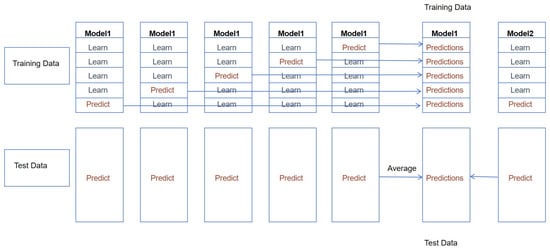 Figure 2. 5-fold cross validation of the base model.
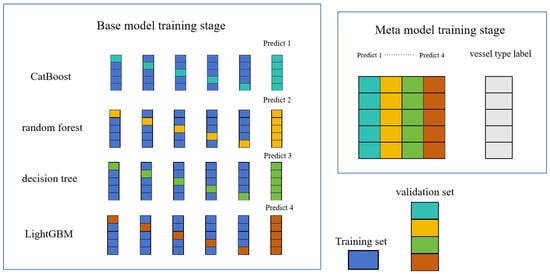 Figure 3. Base model training and meta model training: In the base model training stage, a 5-fold cross validation is conducted sequentially for each base model (CatBoost, Random Forest, Decision Tree, and LightGBM), with a 4-fold split (dark blue) used as for training to learn and another split (sky blue, yellow, green, and orange) used for test prediction, as described in Figure 2. In the meta model training stage, the predicted values of the four base models are used as four “features” to form a matrix of the new training data, which is then handed over to the second-layer model LightGBM for training.In our approach, we use the category with the highest predicted probability as the predicted category.Through this method, the different characteristics and advantages of the base model can be fully utilized, thereby improving the overall performance of the model.
3. Experimental Results and Analysis
3.1. Dataset
The area we are focusing on is Rizhao Port located in China, with latitude coverage from 34° to 36° and longitude from 118° to 120° (Figure 4). The time span is one month, from 1 January 2019 to 31 January 2019. The AIS data used in the study were from satellite systems of ORBCOMM Inc. and IHS Inc. The data used include static and dynamic data, as shown in Table 1 and Table 2. The following figure shows the geographical coverage of the dataset and depicts the location distribution of ships of Rizhao Port.
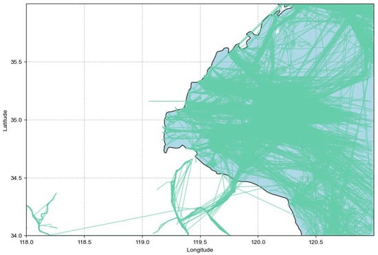
Figure 4.
Ship trajectory of Rizhao Port, China.
3.2. Data Preprocessing
To ensure the accuracy and efficiency of the analysis, data cleaning was initially performed as described in Section 2.2.1. The stability of the trajectory data was then optimized using the unscented Kalman filtering algorithm (Section 2.2.2), ensuring smoothness and better capturing the ship’s motion.
The UKF parameters were optimized for maritime trajectory tracking using scaled Sigma points with = 0.1 to better capture vessel maneuvers (reducing tracking errors by 12% compared to smaller values), = 2.0 for Gaussian systems, and = 1.0 to maintain stable covariance during long-duration tracking.
We begin with 143,470 cleaned dynamic records, which contain features such as latitude, longitude, heading, and speed. To construct meaningful samples, we take 50 consecutive points as a segment (Section 2.2.3).
3.3. Feature Extraction and Fusion
We use the pandas library [54] to read and calculate various features for each segment based on the method outlined in Section 2.3. These features include the average speed, maximum speed, minimum speed, standard deviation of speed, average course, standard deviation of course, average heading, standard deviation of heading, center latitude, and center longitude.
The dynamic features are merged with static features (MMSI, ship type, length, and width) using MMSI as the unique identifier, thereby creating unified ship profiles that encapsulate both behavioral patterns and intrinsic properties. Following data fusion, we implement rigorous completeness checks to eliminate records with missing critical fields, yielding a curated dataset comprising 2911 unique ships. The class distribution exhibits a skewed pattern, with Type 70 ships constituting the dominant class while other categories demonstrate a long-tail distribution characteristic.
We further refine the dataset by selecting the top 5 ship types, ending up with a dataset of 2527 ships. Ships not belonging to the top 5 classes are removed because their low numbers hinder feature capture.
At this point, we have 2527 samples referring to 2527 ships. Each sample contains the following input features: ship length, average speed, maximum speed, minimum speed, speed standard deviation, average course, course standard deviation, average heading, heading standard deviation, center latitude, center longitude, and ship width. The output feature of the ship type has been initially obtained from the AIS and then verified with external data sources. The samples are equipped with MMSI, allowing them to be grouped by ship.
Type 70 ships represent the highest number of ships with 1598, followed by Type 30 ships with a total of 586 ships. The number of ships of Types 80, 52, and 71 is 184, 110, and 49, respectively(Table 3). This data distribution reveals the main composition of different types of ships in the sample.
Table 3.
Top 5 ship types and quantities.
From the given data, we can observe several different types of ships and their corresponding statistical values (Table 4 and Table 5). These datasets roughly provide the operating speed, course, heading, and size characteristics of various types of ships. Here is an analysis of these data.
Table 4.
Dynamic characteristic statistics of different types of ships.
Table 5.
Static characteristic statistics of different types of ships.
- Speed analysisavg_speed: The average speed shows that Type 30 ships have a relatively fast speed of about 2.979 knots, while Type 80 ships have the slowest average speed of only 1.357 knots.max_speed and min_speed: The maximum speed is led by 6.227 knots for Type 30 ships, indicating that this type of ship has a faster speed in the near port area and may have the ability to accelerate and stop quickly. The minimum speed for Type 80 ships is 0.335 knots, which may reflect their limited mobility in certain situations.The standard deviation of Type 30 ships is the highest (1.710), indicating that their speed changes more significantly compared to other types of ships. The standard deviation of Type 80 ships is the lowest (1.095), indicating that their speed is relatively stable.
- Course analysisThe standard deviation of the course for all types of ships is relatively close, ranging from 7.6 to 8.0 degrees, indicating that the variation in the course of ships does not significantly differ with type.
- Location analysiscenter_lat and center_lon: The center latitude and center longitude values represent the central geographic locations of ships, with latitudes ranging from 34.765° to 35.729° and longitudes from 119.304° to 120.571°
- Dimensional analysisShip length and ship width: Type 71 and and Type 80 ships show relatively large average sizes, with average ship lengths of 237.429 m and 165.810 m, respectively, and average ship widths of 33.286 m and 28.272 m, reflecting that they are large ships.For the standard deviation of ship length and ship width, the standard deviation of ship width for Type 30 ships is very high at 12.522, indicating a large range of width variation for this type of ship. The standard deviation of Type 52 ships is the smallest (2.629), indicating that their width is relatively consistent.
- comprehensive analysisType 30 ships are small and flexible ships with a fast average speed and the highest speed variation, which is in line with the general characteristics of Fishing.The size of Type 52 ships is relatively consistent, but there is little change in speed and heading, which is in line with the general characteristics of Tug.Type 70 and Type 80 ships have larger sizes, lower average speeds, and stable speeds, which are large commercial ships such as Cargo or Tanker.Type 71 ships exhibit the highest average size, which is in line with the general characteristics of ships carrying DG, HS, or MP, IMO hazard or pollutant category X.
3.4. Handling Class Imbalance
The number of Type 70 ships is much larger than other types, for example, compared to Type 52, it is almost 15 times that number. If these data are used directly to train the model, their accuracy for Type 70 ships may be high, but their recognition ability for other types, especially Type 52, may be poor.
To overcome this challenge, we adopted SMOTE technology to balance the class distribution (Table 6).
Table 6.
Comparison of the number of ships before and after SMOTE treatment.
To ensure that SMOTE did not adversely affect the feature distribution, we visualized the distribution of key features before and after applying SMOTE. As shown in Figure 5, the distributions of features such as average speed, maximum speed, and minimum speed remained largely unchanged after SMOTE was applied. Specifically, the overall distribution of these features remained stable, with no significant clustering or shifts observed. By comparing the feature distributions before and after SMOTE, we confirmed that the technique effectively increased the number of minority class samples while preserving the original feature distribution. This result indicates that SMOTE successfully addressed class imbalance without introducing unnatural feature changes, ensuring the stability and reliability of model training.
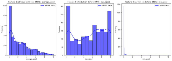
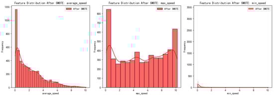
Figure 5.
Distribution of key features before and after applying SMOTE.
3.5. Evaluation Indicators
The classification accuracy is evaluated using the following five indicators: precision, recall, F1 score, ROC Curve, and AUC. The final TP, TN, FP, and FN values for each model are computed by class frequency-weighted averaging of per-category counts, where weights correspond to the proportion of each ship type in the dataset.
- PrecisionPrecision is a measure of the accuracy of a prediction result, representing the proportion of predicted positive categories that are actually positive categories. Its calculation formula is the number of correctly predicted positive samples divided by the total number of predictions that are positive, which means it tells us the proportion of correctly predicted ship types among all predicted ships of that type. The precision can be expressed by the following equation:Among them,TP stands for True Positive: The number of positive classes correctly predicted by the model. For example, Cargo ships correctly classified as Cargo ships.FP stands for False Positive: The number of false positives predicted by the model as positive classes. For example, Non-Cargo ships misclassified as Cargo ships.
- Recall rateRecall rate is an indicator of a model’s ability to identify all positive samples. Its calculation formula is the number of correctly predicted positive samples divided by the actual total number of positive samples. The recall rate can be expressed by the following equation:Among them,TP is as described above.FN stands for False Negativity: The number of negative classes that the model incorrectly predicts. For example, Cargo ships misclassified as Non-Cargo.
- F1 scoreThe F1 score is the harmonic mean of precision and recall, providing a single metric that balances the two, especially useful in imbalanced datasets. This is very helpful when we need to consider two types of errors, namely FP and FN. The F1 score can be expressed by the following equation:The above indicators are usually between 0 and 1, with higher values indicating better performance. Accuracy or recall may be given different importance in various applications.
- ROC CurveThe ROC curve is a graphical representation of a classifier’s ability to distinguish between classes at various thresholds. It plots the True Positive Rate (TPR) against the False Positive Rate (FPR) for different decision thresholds. The ROC curve helps to visualize the trade-off between sensitivity (recall) and specificity (1 − FPR). The ROC curve can be expressed by the following equation:whereTPR (True Positive Rate) is also known as recall.FPR (False Positive Rate) is the fraction of actual negatives that are incorrectly classified as positives.TN stands for true negatives: The number of negative classes correctly predicted by the model. For example, Non-Cargo ships (e.g., Tankers, Tugs) correctly classified as Non-Cargo.
- AUC (Area Under the ROC Curve) AUC measures the area under the ROC curve and is an aggregate measure of a classifier’s ability to distinguish between positive and negative classes. The AUC value ranges from 0 to 1, with higher values indicating better performance. AUC is calculated as the integral of the ROC curve and can be expressed by the following equation:where
- -
- AUC = 1 represents perfect classification.
- -
- AUC = 0.5 represents a random classifier.
- -
- AUC < 0.5 suggests that the model performs worse than random guessing.
A higher AUC value indicates better overall model performance in distinguishing between classes, especially in imbalanced datasets.
3.6. Classification of Ship Type
This section adopts the ensemble classification method based on the stacking strategy introduced in Section 2.6 for ship type classification. This method combines multiple different base models and uses a meta learner to integrate the prediction results of different models. In our case, CatBoost, Random Forest, Decision Tree, and LightGBM are used as the base models, while another LightGBM serves as the final meta model.
Hyperparameters for models were selected based on prior research and empirical performance, with a focus on practical experience. Therefore, we used 5-fold cross-validated grid search to optimize key parameters (e.g., max-depth). The parameters for grid search are provided in Table 7.
Table 7.
Parameters for grid search.
For CatBoost, we used 100 estimators with a learning rate of 0.5 and a maximum depth of 3. Random Forest was set with 100 trees and a maximum depth of 6, following common settings for similar tasks. The Decision Tree was configured with a maximum depth of 6 to balance model complexity and prevent overfitting. For LightGBM, we selected 100 estimators, a learning rate of 0.5, and a maximum depth of 3, based on previous work in the field. The final selections are provided in Table 8.
Table 8.
Chosen hyperparameters of the Ensemble classification method.
The meta model in the stacking Ensemble was also LightGBM, chosen for its efficiency in handling complex relationships. The configuration of LightGBM as the meta model was the same as for the base model, with 100 estimators, a learning rate of 0.5, and a maximum depth of 3.
To verify the performance of the proposed classification model, four different classification models, CatBoost, Random Forest, Decision Tree, and LightGBM, were constructed as comparative experiments.
In addition, we also compared the classification with SVM [26], Neural Network Models [55], and the Ensemble classification method proposed in the current research named MFELCM [39]. MFELCM integrates classifiers such as Random Forest, 1D-CNN, Bi-GRU, and XGBoost, using Random Forest as the final integrator.
The dataset used in all experiments is consistent, with the training set accounting for 70% and the test set accounting for 30%. We used external validation, such as port entry/exit reports, to cross-check and confirm ship types, ensuring that the test data was accurate. For instance, we cross-check ship types by matching information from port entry/exit reports (which include ship type, MMSI, ship name, wharf, and berth) with the MMSI in the test data. If discrepancies in ship types are found, we substitute the test data’s ship type with that from port entry/exit reports. The features have been standardized to eliminate the influence of dimensionality.
Through the Ensemble classification method based on the stacking strategy, we hope that these models can complement each other’s strengths and weaknesses, thereby achieving higher accuracy on the test set. The classification results are as follows:
The significance test (t-test) indicated a significant difference between the two methods (p-value = 0.00035).
Additionally, we conducted experimental validation using AIS data from U.S. coastal waters [56], with two randomly selected days from January 2019 (approximately 9000 ships per day) for training and five randomly selected days from the same month for testing. Through five independent trials, the model achieved mean precision, recall, F1 score, and AUC values of 0.916 (±0.00008), 0.917 (±0.00008), 0.916 (±0.00008), and 0.976 (±0.00003), reaching peak values of 0.931, 0.932, 0.931, and 0.983, respectively. These results indicate strong generalizability across heterogeneous maritime datasets, with the framework maintaining reliable classification accuracy, even with small training samples, while improving computational efficiency. The observed performance suggests practical applicability for real-time classification in maritime monitoring systems.
3.7. Analysis of Experimental Results
3.7.1. Feature Importance
To systematically evaluate feature contributions across multiple ship types while maintaining maritime operational interpretability, we leverage the Shapley values to establish a unified feature importance metric, where each feature’s global impact is decomposed into vessel type-specific contributions—quantifying how static attributes (e.g., ship dimensions) and dynamic behaviors (e.g., speed fluctuations) distinctly influence classification outcomes for Tankers, Cargo, Tugs, and other critical maritime categories.
As illustrated in Figure 6, the Shapley value analysis reveals distinct hierarchical feature impacts across ship type classification. Ship length emerges as the most influential feature, demonstrating universal discriminative power across all ship categories while exhibiting particularly dominant contributions to Type 30 (Fishing) ships. This is closely followed by width. The third critical feature, center latitude, displays geographic operational biases. Dynamic navigation features like maximum speed and speed standard deviation exhibit progressively weaker impacts, underscoring the model’s primary reliance on static features and position. The features of heading, course, and min speed show the least importance.
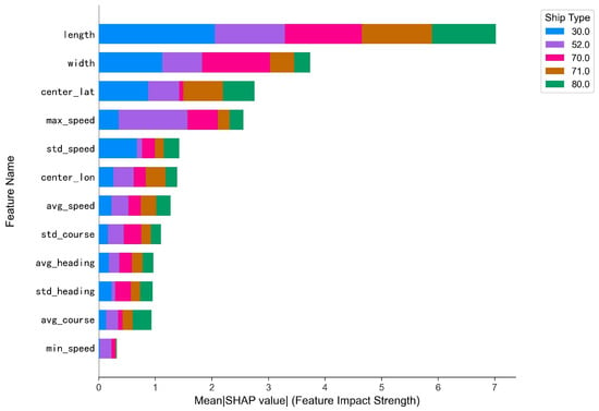
Figure 6.
Mean SHAP value of features.
Notably, ship types exhibit distinct feature affinity patterns as follows: Type 30.0 (blue) dominates contributions across dimensional features (length and width), aligning with Fishing ships’ predictable size ranges. In contrast, Type 52.0 (purple) shows heightened sensitivity to maximum speed thresholds and longitudinal positioning, corresponding to specialized high-speed craft or geographically constrained operations. Other categories (Types 70.0/71.0/80.0) display more uniform feature distributions, suggesting their classification relies on subtle multi-feature synergies rather than individual dominant attributes.
3.7.2. Comparative Analysis of Multiple Classification Methods
According to Figure 7 and Table 9, the ranking of ship type classification results in our research area from good to poor is Ensemble classification method based on a stacking strategy, CatBoost, Random Forest, LightGBM, MFELCM, Decision Tree, Neural Network, and SVM.
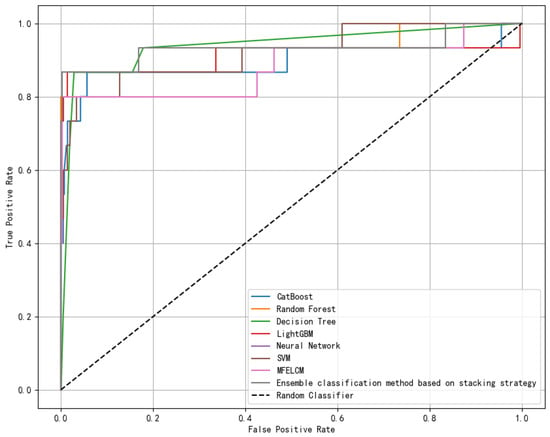
Figure 7.
ROC curve of ship type classification methods’ results.
Table 9.
Comparison of ship type classification Methods Results.
Through the above comparison, we found that CatBoost, Random Forest, Decision Tree, and LightGBM methods are better than SVM and Neural Network, while CatBoost, Random Forest, Decision Tree, and LightGBM are all tree-structured classifiers, indicating that tree-structured classifiers exhibit superior performance in ship type classification. This is consistent with the conclusion proposed in Ref. [26].
Figure 8 and Figure 9 and Table 10 show the results when using ensemble classification models in this work and previous research papers [39]. This Classification Target was chosen to allow for a comparison between this work and previous research papers that used different ensemble classification models with the same dataset in this paper.
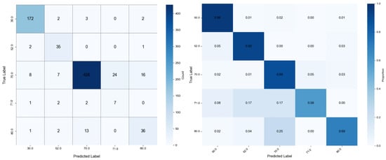
Figure 8.
Confusion matrix results of the Ensemble classification method based on a stacking strategy.
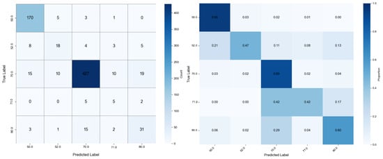
Figure 9.
Confusion matrix results of MFELCM.
Table 10.
Comparison between published results from Ref. [20] and this study.
From the results of these performance indicators, it can be seen that our proposed Ensemble classification method based on a stacking strategy outperforms other methods in all indicators, indicating that after ensemble processing, the variance and bias of individual models are reduced, thereby achieving more stable and accurate results in prediction. The performance of the model has generally improved, which verifies the effectiveness of ensemble classification methods in improving model robustness and prediction ability.
This model performs better for the following reasons:
Diversity: As displayed in the Introduction Section, most researchers focus on a single classifier. Our model integrates multiple types of models, each with unique ways of processing data and assumptions. Their performance or mistakes on different subsets of data are not exactly the same, and this diversity allows this method to leverage the strengths of each model while weakening their weaknesses.
Integrated advantage methods: Unlike existing ensemble classification methods such as MFELCM, we have found through experiments and previous research that tree structure-based classifiers exhibit superior performance in ship type classification. So we choose the tree-structured classifiers as the base model and meta model, which demonstrate higher classification performance than other ensemble models.
Reduced error correlation: Due to the fact that errors between base models are usually not completely correlated, this method can reduce overall errors, especially non systematic errors in model prediction results, by combining models.
Improving generalization ability: Unlike other ensemble models, we use a stacking model. By taking the predictions of multiple models as input, stacking can consider more information and resist overfitting to some extent.
Improving accuracy: Ensemble methods often provides more accurate predictions than any individual model. They can identify the most effective way to combine patterns and achieve higher performance in classification or regression tasks.
Based on the t-test results, we reject the null hypothesis that there is no significant difference between the Ensemble classification method based on a stacking strategy and MFELCM, demonstrating that our model offers superior classification accuracy and stability.
As we can see in Table 11, the training time of our method is 12.97 s, and the training time of CatBoost, Random Forest, and Decision Tree is 1.90 s, 0.71 s, and 0.05 s, respectively, while LightGBM is faster with a speed of only 0.02 s. This increased computational cost is a result of stacking’s inherent structure, which requires training several models before combining their outputs using a meta model. The test time costs of base models and our model are not significantly different, with all being less than 0.1 s. The gap of about 10 s is acceptable for the detection of ship violations. If the trained model is used, the time cost of ship type classification can be almost ignored. Compared with the Neural Network and other ensemble methods, such as MFELCM, our method has more obvious advantages, including high precision and low time costs. However, if the training data are particularly large and the time requirement is quite high, LightGBM and Decision Tree may be better choices. They can achieve relatively good classification accuracy in less than 0.1 s.
Table 11.
Time cost comparison of ship type classification methods.
3.7.3. Analysis of Misclassification Cases
In response to the ship type classification problem with AIS data, we have identified a specific error pattern. Tankers (Type 80) are often misclassified as Cargos (Type 70), with 13 ships being misclassfied from Tankers to Cargos (accounting for 25%). This misclassification can also be seen in other ship type classification studies [2,3,40]. This may indicate that distinguishing between the two can be challenging for such models.
By plotting the trajectories of Cargo and Tanker, we noticed significant overlap in the travel paths of the two types of ships, especially near ports and on major channel (Figure 10).
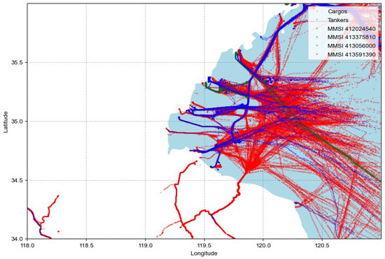
Figure 10.
Ship trajectory with classification error.
In addition, we also focused on several representative ships (MMSI numbers 412024540, 413375810, 413056000, and 413591390) where Tankers are wrongly classified as Cargo ships and we analyzed the features (Table 12).
Table 12.
Features of the ship SHAN XIN (413375810) and Cargo and Tanker ships.
The Tanker (Type 80) SHAN XIN (MMSI 413375810) was misclassified as Cargo (Type 70) due to its features closely resembling those of Cargo ships. Specifically, its average speed (2.267 knots), max speed (9.8 knots), average course (14.133°), and ship dimensions (length: 105 m, width: 17 m) are all more aligned with cargo ships. These characteristics could contribute to its misclassification as Type 70. Although some features, like heading std dev and min speed, are closer to those of Tankers, the overlap in other key metrics makes the distinction between tankers and cargo ships challenging. This overlap in several indicators is a potential reason for the misclassification, highlighting the need for more precise feature differentiation to distinguish the two types.
According to the above research, it is found that the trajectories of Tankers and Cargo ships overlap in terms of travel paths and their features in the model are relatively close; therefore, they are misclassified in this model. However, the overall accuracy of the model is acceptable, which is better than traditional classifiers and the Ensemble classification method. It may be necessary to improve feature engineering and seek more advanced algorithms to enhance the recognition ability of these two types of ship behavior patterns in the future.
4. Conclusions and Future Work
In order to enhance maritime traffic management, this study developed a new ship type classification model using AIS data. Initially, this study collected AIS data from the nearby Rizhao Port in China. Subsequently, through a comprehensive analysis of dynamic and static features, it was found that dynamic features not only reflect the real-time navigation status of ships, but they also reveal their behavioral patterns, while static features provide basic information about ships. The effective combination of the two provides rich information dimensions for the model and enhances its ability to recognize different types of ships. Therefore, combining ship AIS dynamic data and static data, 12 features are extracted from each trajectory for further analysis. After completing data preprocessing, feature extraction, and feature fusion, SMOTE technology is used to solve the problem of class imbalance by synthesizing new minority class samples. Finally, An ensemble classification method based on a stacking strategy is used for ship type classification. Decision Trees, Random Forests, CatBoost, LightGBM, SVM, Neural Networks, and the ensemble methods proposed by other scholars were compared with our method. We used standard classifiers to evaluate the metrics, including precision, recall, F1 score, AUC, and ROC, to assess the performance of the model in five types of ship classification. The evaluation results indicate that the ensemble classification method based on the stacking strategy proposed in this paper outperforms other methods in terms of classification metrics.
The advantage of the ship type classification method proposed in this article is that by extracting ship geometry and trajectory behavior features from AIS data and fully utilizing AIS data information, the performance of the classifier is significantly improved. Through SMOTE technology, the problem of imbalanced ship data has been effectively solved, and the classification accuracy has been improved. In addition, a new ensemble classifier was proposed, which integrates tree structure-based classifiers with advantages in ship type classification, improving classification accuracy. This method provides strong support for ocean monitoring and management, enabling a better response to complex marine environments and diverse ship behaviors.
Finally, although this study has achieved certain results, there are still some limitations. For example, due to their high trajectory similarity, the classification accuracy of Tanker and Cargo ships needs to be further improved. Further exploration of feature selection and model optimization can be used to enhance the classification accuracy of both. In addition, future research can further explore the effects of different combinations of base models to achieve higher classification accuracy. Furthermore, incorporating additional data sources such as environmental factors (e.g., weather and sea conditions) or ship-specific information could improve model performance. Exploring the potential of deep learning methods, including transformers, for sequential data processing might further enhance the classification results.
Author Contributions
Conceptualization, L.D.; methodology, L.D. and L.J.; software, L.D. and S.Y.; validation, L.D.; formal analysis, L.D.; investigation, L.D. and S.Y.; resources, L.D. and L.J.; data curation, L.D., S.Y., and D.G.; writing—original draft preparation, L.D.; writing—review and editing, L.D. and S.Y. All authors have read and agreed to the published version of the manuscript.
Funding
This research received no external funding.
Data Availability Statement
The data used in this study are not publicly available due to privacy and proprietary restrictions. The code is available from the first author upon reasonable request, subject to the relevant confidentiality agreements.
Conflicts of Interest
Author Danyang Geng was employed by the company China Transport Informatics National Engineering Laboratory Co., Ltd. The remaining authors declare that the research was conducted in the absence of any commercial or financial relationships that could be construed as a potential conflict of interest.
References
- Yang, D.; Wu, L.; Wang, S.; Jia, H.; Li, K.X. How big data enriches maritime research—A critical review of Automatic Identification System (AIS) data applications. Transp. Rev. 2019, 39, 755–773. [Google Scholar] [CrossRef]
- Duan, H.; Ma, F.; Miao, L.; Zhang, C. A semi-supervised deep learning approach for vessel trajectory classification based on AIS Data. Ocean Coast. Manag. 2022, 218, 106015. [Google Scholar] [CrossRef]
- Yan, Z.; Song, X.; Zhong, H.; Yang, L.; Wang, Y. Ship classification and anomaly detection based on spaceborne AIS data considering behavior characteristics. Sensors 2022, 22, 7713. [Google Scholar] [CrossRef]
- Rong, H.; Teixeira, A.P.; Soares, C.G. A framework for ship abnormal behavior detection and classification using AIS data. Reliab. Eng. Syst. Saf. 2024, 247, 110105. [Google Scholar] [CrossRef]
- Xie, Z.; Bai, X.; Xu, X.; Xiao, Y. An anomaly detection method based on ship behavior trajectory. Ocean Eng. 2024, 293, 116640. [Google Scholar] [CrossRef]
- Li, H.; Li, W.; Wang, S.; Yang, H.; Guan, J.; Zhang, Y. STAD: Ship trajectory anomaly detection in ocean with dynamic pattern clustering. Ocean Eng. 2024, 313, 119530. [Google Scholar] [CrossRef]
- Gao, M.; Shi, G. Ship-handling behavior pattern recognition using AIS sub-trajectory clustering analysis based on the T-SNE and spectral clustering algorithms. Ocean Eng. 2020, 205, 106919. [Google Scholar] [CrossRef]
- Cai, Z.; Fan, Q.; Li, L.; Yu, L.; Li, C. An efficient Meta-VSW method for ship behaviors recognition and application. Ocean Eng. 2024, 311, 118870. [Google Scholar] [CrossRef]
- Xin, R.; Pan, J.; Yang, F.; Yan, X.; Ai, B.; Zhang, Q. Graph deep learning recognition of port ship behavior patterns from a network approach. Ocean Eng. 2024, 305, 117921. [Google Scholar] [CrossRef]
- Leeuwen, B.; Nutzel, M. Detecting drug transfers via the drop-off method: A supervised model approach using AIS data. Mach. Learn. Appl. 2024, 18, 100590. [Google Scholar] [CrossRef]
- Liu, J.; Li, J.; Liu, C. AIS-based kinematic anomaly classification for maritime surveillance. Ocean Eng. 2024, 305, 118026. [Google Scholar] [CrossRef]
- Chen, Y.; Qi, X.; Huang, C.; Zheng, J. A data fusion method for maritime traffic surveillance: The fusion of AIS data and VHF speech information. Ocean Eng. 2024, 311, 118953. [Google Scholar] [CrossRef]
- Liu, C.; Li, S.; Chen, S.; Chen, Q.; Liu, K. Research on the navigational risk of liquefied natural gas carriers in an inland river based on entropy: A cloud evaluation model. Transp. Saf. Environ. 2024, 6, tdad018. [Google Scholar] [CrossRef]
- Bai, X.; Cheng, L.; Iris, Ç. Data-driven financial and operational risk management: Empirical evidence from the global tramp shipping industry. Transp. Res. Part E Logist. Transp. Rev. 2022, 158, 102617. [Google Scholar] [CrossRef]
- Yang, T.; Wang, X.; Liu, Z. Ship Type Recognition Based on Ship Navigating Trajectory and Convolutional Neural Network. J. Mar. Sci. Eng. 2022, 10, 84. [Google Scholar] [CrossRef]
- McCauley, D.J.; Woods, P.; Sullivan, B.; Bergman, B.; Jablonicky, C.; Roan, A.; Hirshfield, M.; Boerder, K.; Worm, B. Ending hide and seek at sea. Science 2016, 351, 1148–1150. [Google Scholar] [CrossRef]
- Surucu-Balci, E.; Iris, Ç.; Balci, G. Digital information in maritime supply chains with blockchain and cloud platforms: Supply chain capabilities, barriers, and research opportunities. Technol. Forecast. Soc. Chang. 2024, 198, 122978. [Google Scholar] [CrossRef]
- Oliveira, P.; Silva, M. Detecting illegal fishing activities using vessel identification and tracking data. Mar. Policy 2020, 121, 103–110. [Google Scholar]
- Salerno, E. Using low-resolution SAR scattering features for ship classification. IEEE Geosci. Remote Sens. Lett. 2022, 19, 1–4. [Google Scholar] [CrossRef]
- Dong, Y.; Xu, K.; Zhu, C.; Guan, E.; Liu, Y. E-FPN: Evidential feature pyramid network for ship classification. Remote Sens. 2023, 15, 3916. [Google Scholar] [CrossRef]
- Huang, L.; Wang, F.; Zhang, Y.; Xu, Q. Fine-grained ship classification by combining CNN and Swin Transformer. Remote Sens. 2022, 14, 3087. [Google Scholar] [CrossRef]
- Chen, J.; Chen, K.; Chen, H.; Li, W.; Zou, Z.; Shi, Z. Contrastive Learning for fine-grained ship classification in remote sensing images. IEEE Trans. Geosci. Remote Sens. 2022, 60, 1–16. [Google Scholar] [CrossRef]
- Yang, S.; Zhang, X.; Zhao, W.; Hu, Q.; Luo, H.; Liu, C.; Peng, J. DSNet: Dual-stream network for fine-grained ship classification in optical remote sensing images. Remote Sens. Lett. 2024, 15, 792–804. [Google Scholar] [CrossRef]
- Chen, X.; Zheng, J.; Li, C.; Wu, B.; Wu, H.; Montewka, J. Maritime traffic situation awareness analysis via high-fidelity ship imaging trajectory. Multimed. Tools Appl. 2024, 83, 48907–48923. [Google Scholar] [CrossRef]
- Chen, L.; Wang, Q.; Zhu, E.; Feng, D.; Wu, H.; Liu, T. Ship fine-grained classification network based on multi-scale feature fusion. Ocean Eng. 2025, 318, 120079. [Google Scholar] [CrossRef]
- Huang, I.L.; Lee, M.C.; Nieh, C.Y.; Huang, J.C. Ship classification based on AIS data and machine learning methods. Electronics 2023, 13, 98. [Google Scholar] [CrossRef]
- Amigo, D.; Pedroche, D.S.; García, J.; Molina, J.M. Segmentation optimization in trajectory-based ship classification. J. Comput. Sci. 2022, 59, 101568. [Google Scholar] [CrossRef]
- Luo, P.; Gao, J.; Wang, G.; Han, Y. Research on Ship Classification Method Based on AIS Data. In Proceedings of the Computer Supported Cooperative Work and Social Computing: 15th CCF Conference, ChineseCSCW 2020, Shenzhen, China, 7–9 November 2020; pp. 222–236. [Google Scholar]
- Yan, Z.; Song, X.; Yang, L.; Wang, Y. Ship classification in synthetic aperture radar images based on multiple classifiers ensemble learning and Automatic Identification System Data Transfer Learning. Remote Sens. 2022, 14, 5288. [Google Scholar] [CrossRef]
- Lang, H.; Yang, G.; Li, C.; Xu, J. Multisource heterogeneous transfer learning via feature augmentation for ship classification in sar imagery. IEEE Trans. Geosci. Remote Sens. 2022, 60, 1–14. [Google Scholar] [CrossRef]
- De Souza, E.N.; Boerder, K.; Matwin, S.; Worm, B. Correction: Improving fishing pattern detection from satellite AIS using data mining and machine learning. PLoS ONE 2016, 11, e0163760. [Google Scholar] [CrossRef]
- Guan, Y.; Zhang, J.; Zhang, X.; Li, Z.; Meng, J.; Liu, G.; Cao, C. Identification of fishing vessel types and analysis of seasonal activities in the northern South China Sea based on AIS DATA: A case study of 2018. Remote Sens. 2021, 13, 1952. [Google Scholar] [CrossRef]
- Cheng, X.; Zhang, F.; Chen, X.; Wang, J. Application of artificial intelligence in the study of Fishing Vessel behavior. Fishes 2023, 8, 516. [Google Scholar] [CrossRef]
- Nugraha, R.A.; Pardede, H.F.; Subekti, A. Oversampling based on generative adversarial networks to overcome imbalance data in predicting fraud insurance claim. Kuwait J. Sci. 2022, 49, 1–12. [Google Scholar] [CrossRef]
- An, Q.; Huang, S.; Han, Y.; Zhu, Y. Ensemble learning method for classification: Integrating data envelopment analysis with machine learning. Comput. Oper. Res. 2024, 169, 106739. [Google Scholar] [CrossRef]
- Zhang, H.; Liu, C.; Ma, J.; Sun, H. Time-prior-based stacking ensemble deep learning model for ship infrared automatic target recognition in complex maritime scenarios. Infrared Phys. Technol. 2024, 137, 105168. [Google Scholar] [CrossRef]
- Chan, Y.T. Ensemble learning-based method for maritime background subtraction in open sea environments. Comput. Vis. Image Underst. 2024, 238, 103859. [Google Scholar] [CrossRef]
- Chen, X.; Chen, W.; Wu, B.; Wu, H.; Xian, J. Ship visual trajectory exploitation via an ensemble instance segmentation framework. Ocean Eng. 2024, 313, 119368. [Google Scholar] [CrossRef]
- Wang, Y.; Yang, L.; Song, X.; Chen, Q.; Yan, Z. A multi-feature ensemble learning classification method for ship classification with space-based AIS Data. Appl. Sci. 2021, 11, 10336. [Google Scholar] [CrossRef]
- Meyer, R.; Kleynhans, W. Vessel classification using AIS data. Ocean Eng. 2025, 319, 120043. [Google Scholar] [CrossRef]
- Luo, D.; Chen, P.; Yang, J.; Li, X.; Zhao, Y. A New Classification Method for Ship Trajectories Based on AIS Data. J. Mar. Sci. Eng. 2023, 11, 1646. [Google Scholar] [CrossRef]
- MMSI Mid Codes. Available online: https://www.vtexplorer.com/mmsi-mid-codes-en/ (accessed on 6 March 2024).
- Chen, Y.; Chen, Y.; Cui, Y.; Cai, X.; Yin, C.; Cheng, Y. Optimizing vessel trajectories: Advanced denoising and interpolation techniques for AIS data. Ocean Eng. 2025, 327, 120988. [Google Scholar] [CrossRef]
- Kalman, E.R. A New Approach to Linear Filtering and Prediction Problems. J. Artif. Intell. Res. 1960, 82, 35–45. [Google Scholar] [CrossRef]
- Cole, B.; Schamberg, G. Unscented Kalman filter for long-distance vessel tracking in geodetic coordinates. Appl. Ocean Res. 2022, 124, 103205. [Google Scholar] [CrossRef]
- FilterPy: A Python Library for Kalman Filtering and Optimal Estimation. Available online: https://github.com/rlabbe/filterpy (accessed on 21 June 2024).
- Tetreault, B.J. Use of the Automatic Identification System (AIS) for Maritime Domain Awareness (MDA). In Proceedings of the OCEANS 2005 MTS/IEEE, Washington, DC, USA, 17–23 September 2005; pp. 1–5. [Google Scholar]
- Sánchez Pedroche, D.; Amigo, D.; García, J.; Molina, J.M. Architecture for trajectory-based fishing ship classification with AIS Data. Sensors 2020, 20, 3782. [Google Scholar] [CrossRef]
- Chawla, N.V.; Bowyer, K.W.; Hall, L.O.; Kegelmeyer, W.P. SMOTE: Synthetic minority over-sampling technique. J. Artif. Intell. Res. 2022, 16, 321–357. [Google Scholar] [CrossRef]
- Zilali, A.; Adda, M.; Ziane, K.; Berger, M. Machine learning-based state of charge estimation: A comparison between CatBoost model and C-BLSTM-AE model. Mach. Learn. Appl. 2025, 20, 100629. [Google Scholar] [CrossRef]
- Breiman, L. Random forests. Mach. Learn. 2001, 45, 5–32. [Google Scholar] [CrossRef]
- Quinlan, J.R. Induction of decision trees. Mach. Learn. 1986, 1, 81–106. [Google Scholar] [CrossRef]
- Ke, G.; Meng, Q.; Finley, T.; Wang, T.; Chen, W.; Ma, W.; Liu, T.Y. LightGBM: A highly efficient gradient boosting decision tree. In Proceedings of the Advances in Neural Information Processing Systems, Long Beach, CA, USA, 4–9 December 2017; pp. 3146–3154. [Google Scholar]
- McKinney, W. Data structures for statistical computing in Python. In Proceedings of the 9th Python in Science Conference, Austin, TX, USA, 28 June–3 July 2010; pp. 51–56. [Google Scholar]
- Ghiassi, M.; Burnley, C. Measuring effectiveness of a dynamic artificial neural network algorithm for classification problems. Expert Syst. Appl. 2025, 37, 3118–3128. [Google Scholar] [CrossRef]
- The U.S. Marine Cadastre AIS Dataset. Available online: https://marinecadastre.gov/ais/ (accessed on 18 April 2025).
Disclaimer/Publisher’s Note: The statements, opinions and data contained in all publications are solely those of the individual author(s) and contributor(s) and not of MDPI and/or the editor(s). MDPI and/or the editor(s) disclaim responsibility for any injury to people or property resulting from any ideas, methods, instructions or products referred to in the content. |
© 2025 by the authors. Licensee MDPI, Basel, Switzerland. This article is an open access article distributed under the terms and conditions of the Creative Commons Attribution (CC BY) license (https://creativecommons.org/licenses/by/4.0/).