Enhancing Trajectory Tracking Performance of Underwater Gliders Using Finite-Time Sliding Mode Control Within a Reinforcement Learning Framework

Abstract

Underwater gliders, as autonomous underwater vehicles, are integral to oceanographic research, environmental monitoring, and military applications. Given the intricate and ever-changing underwater environment, the precise management of an underwater glider’s dive depth and pitch angle is imperative for optimal functionality.This study introduces a finite-time sliding mode control method for controlling dive depth and pitch angle of underwater gliders. It incorporates a radial basis function neural network in a critic–actor reinforcement learning framework, enhancing navigational performance in difficult conditions. Sea trial data are used to create a dynamic model for the underwater glider, which is then used to design a control law. Sliding mode control is used to align the dive depth and pitch angle with the desired trajectory. Actor and critic neural networks are used to handle disturbances and evaluate error costs. By incorporating standard deviation update technique into actor and critic neural networks, along with weight updates, we improve controller stability and reduce errors in maintaining dive depth and pitch angle. Our approach is proven to be more effective than traditional SMC and reinforcement learning SMC methods in trajectory tracking, even in the presence of disturbances, as shown in the simulation results.

1. Introduction

Underwater exploration is a frontier field in marine science and technology, playing a vital role in resource discovery, environmental monitoring, and ecological research [1,2,3]. In the face of global climate change and rising demand for marine resources, this field presents both significant opportunities and complex challenges. Common platforms include Remotely Operated Vehicles (ROVs), Autonomous Underwater Vehicles (AUVs), and underwater gliders [4,5]. ROVs and AUVs, propelled by thrusters, offer high maneuverability and precise control, making them suitable for tasks such as maintenance, salvage operations, and scientific exploration. In contrast, underwater gliders achieve propulsion through variable buoyancy and hydrodynamic lift, enabling slower yet more energy-efficient movement [6]. Their low noise and extended range make them ideal for long-duration marine monitoring missions.

Despite these advantages, underwater gliders face challenges such as environmental disturbances and unmodeled dynamics [7,8], necessitating advanced control algorithms for precise and reliable operation. Early studies primarily employed conventional control strategies, including Proportional-Integral-Derivative (PID) and Linear Quadratic Regulator (LQR) control. Leonard et al. [9] developed a LQR controller based on a linearized system model, enabling accurate vertical trajectory tracking. Liu et al. [10] demonstrated the effectiveness of PID control in regulating the depth and pitch angle. Wu et al. later validated the applicability of the LQR method for basic motion control, though their results showed that heading adjustment from −1.5 to 1.5 rad required approximately 1000 s, while pitch angle control reached the target within 30 s.

As traditional methods struggle with dynamic and nonlinear underwater environments, modern control strategies—such as adaptive, robust, and sliding mode control—have been introduced. Adaptive control is particularly valued for its real-time parameter adjustment capability [11]. Wan et al. [12] applied an adaptive extended state observer in shallow-water navigation, while Sang et al. [13] implemented a fuzzy PID controller for heading tracking. Robust control methods, known for their disturbance rejection, have also gained traction. Nguyen et al. and Garc’ıa et al. [14,15] proposed robust adaptive controllers for heading stabilization, although these methods depended heavily on accurate system modeling.

In parallel, sliding mode control techniques have been explored for their effectiveness in trajectory tracking [16,17]. Zhang et al. [18] proposed an adaptive non-singular integral terminal sliding mode control (ANITSMC) method, which ensures finite-time convergence and robust performance under a bounded range of external disturbances. Zhou et al. [19] developed an adaptive robust sliding mode approach to counter parameter uncertainties, though the well-known chattering problem remains a concern. Zou et al. [20] further improved upon this by proposing a non-singular fast-terminal sliding mode controller for fixed-time tracking. Meanwhile, Gupta Roy et al. [21] presented variants of the sliding mode and active disturbance rejection control (ADRC), demonstrating advantages in energy efficiency and disturbance rejection.

In contemporary control system research, data-driven methodologies, including neural network control and reinforcement learning (RL), are increasingly recognized as state-of-the-art technologies for tackling complex control challenges. These innovative approaches demonstrate remarkable adaptability and intelligence, particularly within precision control systems such as underwater gliders. Recent studies have reported substantial advancements in this field. For instance, Juan et al. introduced a Heterogeneous Agent Asynchronous Policy Gradient (HAAPG) method grounded in model-free reinforcement learning, which achieves high-precision motion control by dynamically adjusting the rotation of a movable mass block to effectively counteract external disturbances [22]. Simultaneously, Wang and colleagues developed an adaptive sliding mode fault-tolerant controller that marked a significant advancement in addressing the modeling uncertainties of underwater gliders, achieving a mean integral absolute error of 0.29 and a convergence time of 24.64 s [23]. Notably, the advancement of neural network-based control technologies has garnered significant scholarly attention. Lei et al. successfully combined physical modeling principles with data-driven methodologies, thereby markedly improving the modeling accuracy of underwater gliders [24]. Building upon this foundation, Jeong and Gao introduced a neural network-based self-tuning PID controller and a model-free neural adaptive attitude control strategy, both of which exhibited robust control stability under uncertain conditions [25,26]. These methodologies are characterized by their ability to effectively learn and interpret nonlinear system behaviors, demonstrating enhanced perception and adaptability in complex dynamic systems [27]. Furthermore, the research conducted by Su and Zang underscores the potential of reinforcement learning in tasks related to attitude control and heading tracking [28,29]. By integrating traditional control strategies, such as PID control, with sophisticated machine learning algorithms, researchers are progressively addressing the limitations inherent in conventional control systems.

Recent advancements in sensing and communication technologies have markedly enhanced the performance of underwater glider control systems. In particular, the high-precision fiber-optic sensing technology introduced by Jawad Mirza et al. plays a pivotal role in augmenting the disturbance rejection capabilities and stability of data-driven control algorithms [30,31]. Complementary to this, Wang et al. have developed a cooperative data compression and communication strategy for underwater oil spill detection, employing support vector machines and density-based spatial clustering techniques [32]. Concurrently, significant progress has been achieved in the domain of trajectory tracking control strategies. A range of methodologies—including quadratic programming, PID control, and sliding mode control—have been rigorously investigated and implemented across various fields such as ground vehicles, unmanned aerial vehicles (UAVs), and surface vessels [33]. The fundamental principles underlying these methods—such as dynamic response optimization, enhanced disturbance rejection, and robust system design—offer substantial insights and advancements.

Based on the literature reviewed, it is clear that current control methods for underwater gliders encounter several significant challenges, such as slow response times, limited disturbance rejection capabilities, and inadequate adaptability to dynamic environments. To address these challenges, this paper introduces a SMC strategy enhanced by Critic–Actor Reinforcement Learning with Standard Deviation updating (SD-RLSMC). The primary innovations of this approach include the following:

1

Precise hydrodynamic parameter identification and dynamic modeling: Hydrodynamic parameters are accurately identified using the Trust Region Reflective Algorithm, based on experimental data obtained from the South China Sea. A dynamic model is subsequently established, incorporating a depth correction term and nonlinear hydrodynamic effects. The model’s accuracy is validated by comparing the root-mean-square error (RMSE) between the proposed full-order model and experimental results.

2

Critic–actor reinforcement learning framework with radial basis function neural networks: Radial Basis Function (RBF) neural networks are embedded within a critic–actor reinforcement learning framework to construct a unified perturbation estimation model, enabling the real-time approximation of unmodeled dynamics and external disturbances. Compared to conventional sliding mode control, the proposed SD-RLSMC approach reduces the RMSE by approximately 42% in disturbance rejection scenarios and substantially enhances trajectory tracking performance.

3

Standard deviation adjustment: An adaptive standard deviation updating mechanism based on gradient descent is introduced to dynamically regulate the local approximation capability of RBF neural networks. This mechanism improves the approximation accuracy for complex nonlinear systems, enhances controller adaptability under varying environmental conditions, and reduces the required control effort.

The remainder of this paper is organized as follows: Section 2 presents the dynamic modeling and hydrodynamic parameter identification of the underwater glider. Section 3 introduces a finite-time sliding mode control strategy based on reinforcement learning. Section 4 evaluates the proposed controller’s performance through numerical simulations. Finally, Section 5 concludes the paper and outlines potential directions for future research.

2. Dynamic Modeling and Parameter Identification

In this section, a dynamic model of the underwater glider is proposed for controller design. A parameter identification methodology is applied to acquire the hydrodynamic coefficients, rotational inertia, and other relevant parameters. The model’s accuracy is confirmed through validation with additional data.

2.1. Model Description

Figure 1 displays a schematic diagram of an underwater glider, along with its vertical plane coordinate system. In accordance with Fossen’s definition, the movement and location of an underwater glider can be characterized with the following two coordinate systems: the inertial coordinate system and the body-fixed coordinate system [34].

To formulate a dynamic model for tracking vertical plane trajectories, the following assumptions shall be established [35]:

1

The center of buoyancy is typically considered to be fixed, a condition supported by the glider’s structural symmetry and inherent hydrostatic stability. However, in practical scenarios, minor shifts in the center of buoyancy may occur due to fluid disturbances or structural deformations. These shifts are generally small in magnitude, evolve gradually, and can therefore be treated as bounded, unmodeled dynamic perturbations.

2

The influence of actuator motion on mass distribution is negligible. The glider’s actuators, such as the buoyancy and attitude adjustment units, operate slowly and have a limited capacity for mass adjustments, resulting in minimal dynamic impact on the overall mass distribution. Any unmodeled perturbations can be incorporated into the bounded uncertainty analysis.

3

The pitch angle $\theta$ is constrained between $-\pi /\phantom{\pi 2}2$ and $\pi /\phantom{\pi 2}2$ to prevent the occurrence of inverted or runaway gliders in the vertical plane. In practice, the physical limitations of the actuators, such as the operational range of the hydraulic pump, along with stability requirements, ensure that the pitch angle remains within this range. Exceeding this range may lead to control failures or complicate the dynamic behavior.

When we focus on the motion of an underwater glider in the vertical plane, a simplified dynamic model can be obtained according to the literature [20,36,37]:

$$\left\{\begin{array}{c}\dot{z}\left(t\right)=-v_1\left(t\right)sin\left(\theta \left(t\right)\right)+v_3\left(t\right)cos\left(\theta \left(t\right)\right)\hfill \\ \dot{\theta }\left(t\right)=q\left(t\right)\hfill \\ \dot{q}\left(t\right)=M+B{r}_{\mathrm{p}1}\left(t\right)\hfill \\ {\dot{v}}_1\left(t\right)={\displaystyle \frac{1}{M_{\mathrm{f}1}+m\left(t\right)}}\left(F_1+F_2+F_3\right)\hfill \\ {\dot{v}}_3\left(t\right)={\displaystyle \frac{1}{M_{\mathrm{f}3}+m\left(t\right)}}\left(F_4+F_5\right)\hfill \end{array}\right.$$

(1)

where the following holds:

$$\begin{array}{cc}\hfill F_1& =-q\left(t\right)v_3\left(t\right)\left(M_{\mathrm{f}3}+m\left(t\right)\right)-\dot{q}\left(t\right)m_{\mathrm{p}}{r}_{\mathrm{p}3}\hfill \\ \hfill F_2& =-D\left(t\right)cos\left(\alpha \right(t\left)\right)+L\left(t\right)sin\left(\alpha \right(t\left)\right)\hfill \\ \hfill F_3& =-m_{0}gsin\left(\theta \left(t\right)\right)+q^2\left(t\right)\left(m_{\mathrm{p}}{r}_{\mathrm{p}1}\left(t\right)+m_{\mathrm{b}}\left(t\right)r_{\mathrm{b}1}\right)\hfill \\ \hfill F_4& =-D\left(t\right)sin\left(\alpha \right(t\left)\right)-L\left(t\right)cos\left(\alpha \right(t\left)\right)\hfill \\ \hfill F_5& =m_{0}gcos\left(\theta \left(t\right)\right)+q\left(t\right)v_1\left(t\right)\left(M_{\mathrm{f}1}+m\left(t\right)\right)\hfill \\ \hfill M& ={\displaystyle \frac{1}{E}}\left(T_2\left(t\right)-M_{\mathrm{b}}{r}_{\mathrm{b}1}gcos\left(\theta \left(t\right)\right)-m_{\mathrm{p}}{r}_{\mathrm{p}3}gsin\left(\theta \left(t\right)\right)+v_1\left(t\right)v_3\left(t\right)(M_{\mathrm{f}3}-M_{\mathrm{f}1}-m_{\mathrm{p}})\right.\hfill \\ \hfill & -\left.\left({\dot{v}}_1\left(t\right)+v_1\left(t\right)q\left(t\right)\right)m_{\mathrm{p}}{r}_{\mathrm{p}3}+{\dot{v}}_3\left(t\right)m_{\mathrm{b}}{r}_{\mathrm{b}1}-v_1\left(t\right)q\left(t\right)m_{\mathrm{b}}{r}_{\mathrm{b}1}\right)\hfill \\ \hfill B& ={\displaystyle \frac{1}{E}}\left(-m_{\mathrm{p}}gcos\left(\theta \left(t\right)\right)+{\dot{v}}_3\left(t\right)m_{\mathrm{p}}-v_1\left(t\right)q\left(t\right)m_{\mathrm{p}}-2q\left(t\right)m_{\mathrm{p}}{\dot{r}}_{\mathrm{p}1}\left(t\right)\right)\hfill \end{array}$$

In addition, the velocities in the body-fixed coordinate system are represented by $v_1\left(t\right)$, $v_3\left(t\right)$, and $q\left(t\right)$. The values of $v_1\left(t\right)$ and $v_3\left(t\right)$ can be obtained through inertial measurement unit (IMU) sensors. The variables $z\left(t\right)$ and $\theta \left(t\right)$ correspond to the submersion depth and pitch angle of the inertial coordinate system, respectively. The total mass of the glider can be calculated by $m\left(t\right)=m_{\mathrm{rb}}+m_{\mathrm{p}}+m_{\mathrm{b}}\left(t\right)$, where $m_{\mathrm{rb}}$ represents the glider body weight. The equation $m_0=m\left(t\right)-m_{\mathrm{d}}$ represents the net buoyancy of the glider, where $m_{\mathrm{d}}$ denotes the displacement mass, $m_{\mathrm{p}}$ represents the attitude adjustment mass, and g is the acceleration of gravity. The variable ballast mass is located at position $r_{\mathrm{b}1}$ along the x-axis in the body-fixed coordinate system, while $r_{\mathrm{p}3}$ indicates the position of the internal mass along the x-axis in the same coordinate system. Furthermore, $M_{\mathrm{f}1}$ and $M_{\mathrm{f}3}$ pertain to the additional mass. The variable $r_{\mathrm{p}1}\left(t\right)$ denotes the position of the attitude adjustment unit, while $m_{\mathrm{b}}\left(t\right)$ represents the mass of the buoyancy adjustment unit. These two variables serve as the control inputs for the dynamics model. The hydraulic pump is used to control the injection (or extraction) of seawater into (or out of) the bladder, allowing for precise control over the buoyancy unit’s mass.

It is wel -documented in Ref. [38] that the buoyancy regulation mass, $m_{\mathrm{b}}\left(t\right)$, is influenced by both seawater density and pressure. To simplify the calculation of the buoyancy, the effect of the changes in seawater density and pressure is combined by incorporating a depth correction term into the buoyancy regulation mass. Consequently, the buoyancy regulation mass can be expressed as follows:

$$m_{\mathrm{b}}\left(t\right)=\pm \left({\rho }_{\mathrm{sea}}{V}_{\mathrm{sea}}+K_{\mathrm{h}}z\right)$$

(2)

where ${\rho }_{\mathrm{sea}}$ is the density of seawater, set in this research as $1022.70\mathrm{kg}/\phantom{\mathrm{kg}{\mathrm{m}}^3}{\mathrm{m}}^3$.

$K_{\mathrm{h}}$, denoted as a correction term, accounts for the impact of depth on the buoyancy regulation. Moreover, the variables $\alpha \left(t\right)$, $D\left(t\right)$, $L\left(t\right)$, $T_2\left(t\right)$, and E represent the angle of attack, drag, lift, pitching moment, and velocity, respectively, which are mathematically expressed as follows:

$$\left\{\begin{array}{c}\alpha \left(t\right)=arctan\left({\displaystyle \frac{v_3\left(t\right)}{v_1\left(t\right)}}\right)\hfill \\ V\left(t\right)=\sqrt{v_1^2\left(t\right)+v_3^2\left(t\right)}\hfill \\ D\left(t\right)=\left(K_{\mathrm{D}0}+K_{\mathrm{D}}{\alpha }^2\left(t\right)\right)V^2\left(t\right)\hfill \\ L\left(t\right)=\left(K_{\mathrm{L}0}+K_{\mathrm{L}}\alpha \left(t\right)\right)V^2\left(t\right)\hfill \\ T_2\left(t\right)=\left(K_{\mathrm{M}0}+K_{\mathrm{M}}\alpha \left(t\right)+K_{\mathrm{q}}q\left(t\right)\right)V^2\left(t\right)\hfill \\ J_2=J_{\mathrm{rb}2}+J_{\mathrm{f}2}\hfill \\ E=J_2+m_{\mathrm{p}}{r}_{\mathrm{p}3}^2+m_{\mathrm{b}}\left(t\right)r_{\mathrm{b}1}^2\hfill \end{array}\right.$$

(3)

where $K_{\mathrm{D}0}$, $K_{\mathrm{D}}$, $K_{\mathrm{L}0}$, $K_{\mathrm{L}}$, $K_{\mathrm{M}0}$, $K_{\mathrm{M}}$, $K_{\mathrm{q}}$, and $J_2$ are the hydrodynamic parameters and inertial moment. These parameters, along with $K_{\mathrm{h}}$, will be identified with sea trial data.

It is anticipated that the underwater glider will adhere to the desired trajectory in terms of the diving depth and pitch angle. Different from the research by Zou [20], the current study involves the doubling of both control inputs and outputs, leading to a more intricate model. This model exhibits significant nonlinear characteristics and dynamic behaviors, underscoring the necessity for an advanced controller design. Given the relatively low and predominantly stable velocity of the underwater glider (ranging from 0.5 to 0.8 knots), it is reasonable to disregard the impact of velocity variation in Equation (1). Moreover, the expression for energy, represented as $J_2+m_{\mathrm{b}}{r}_{\mathrm{b}1}^2\gg m_{\mathrm{b}}\left(t\right)r_{\mathrm{b}1}^2$, can be simplified to $E=J_2+m_{\mathrm{b}}{r}_{\mathrm{b}1}^2$. Thus, Equation (1) can be expressed more succinctly as follows:

$$\left\{\begin{array}{cc}\hfill \dot{z}\left(t\right)& =-v_1\left(t\right)sin\theta \left(t\right)+v_3\left(t\right)cos\theta \left(t\right)\hfill \\ \hfill \dot{\theta }\left(t\right)& =q\left(t\right)\hfill \\ \hfill \dot{q}\left(t\right)& =M(\theta \left(t\right),\dot{\theta }\left(t\right))+B(\theta \left(t\right),\dot{\theta }\left(t\right))u_2\left(t\right)\hfill \\ \hfill {\dot{v}}_1\left(t\right)& ={\displaystyle \frac{1}{M_{\mathrm{f}1}}}\left[\begin{array}{c}-q\left(t\right)v_3\left(t\right)M_{\mathrm{f}3}-D\left(t\right)cos\alpha \left(t\right)+L\left(t\right)sin\alpha \left(t\right)\\ -m_{0}gsin\theta \left(t\right)+q{\left(t\right)}^2\left(m_{\mathrm{p}}{r}_{\mathrm{p}1}\left(t\right)+m_{\mathrm{b}}\left(t\right)r_{\mathrm{b}1}\right)\end{array}\right]\hfill \\ \hfill {\dot{v}}_3\left(t\right)& ={\displaystyle \frac{1}{M_{\mathrm{f}3}}}\left[\begin{array}{c}q\left(t\right)v_1\left(t\right)M_{\mathrm{f}1}-D\left(t\right)sin\alpha \left(t\right)\\ -L\left(t\right)cos\alpha \left(t\right)+m_{0}gcos\theta \left(t\right)\end{array}\right]\hfill \end{array}\right.$$

(4)

where the functions $M(·)$ and $B(·)$ are defined as follows:

$$\begin{array}{cc}\hfill M(\theta \left(t\right),\dot{\theta }\left(t\right))& ={\displaystyle \frac{1}{E}}[T_2\left(t\right)-m_{\mathrm{b}}{r}_{\mathrm{b}1}gcos\theta \left(t\right)-m_{\mathrm{p}}{r}_{\mathrm{p}3}gsin\theta \left(t\right)\hfill \\ \hfill & +v_1\left(t\right)v_3\left(t\right)\left(M_{\mathrm{f}3}-M_{\mathrm{f}1}-m_{\mathrm{p}}\right)-v_1\left(t\right)q\left(t\right)m_{\mathrm{p}}{r}_{\mathrm{p}3}-v_1\left(t\right)q\left(t\right)m_{\mathrm{b}}{r}_{\mathrm{b}1}]\hfill \\ \hfill B(\theta \left(t\right),\dot{\theta }\left(t\right))& ={\displaystyle \frac{1}{E}}\left(-m_{\mathrm{p}}gcos\theta \left(t\right)-m_{\mathrm{p}}{v}_1\left(t\right)q\left(t\right)\right)\hfill \end{array}$$

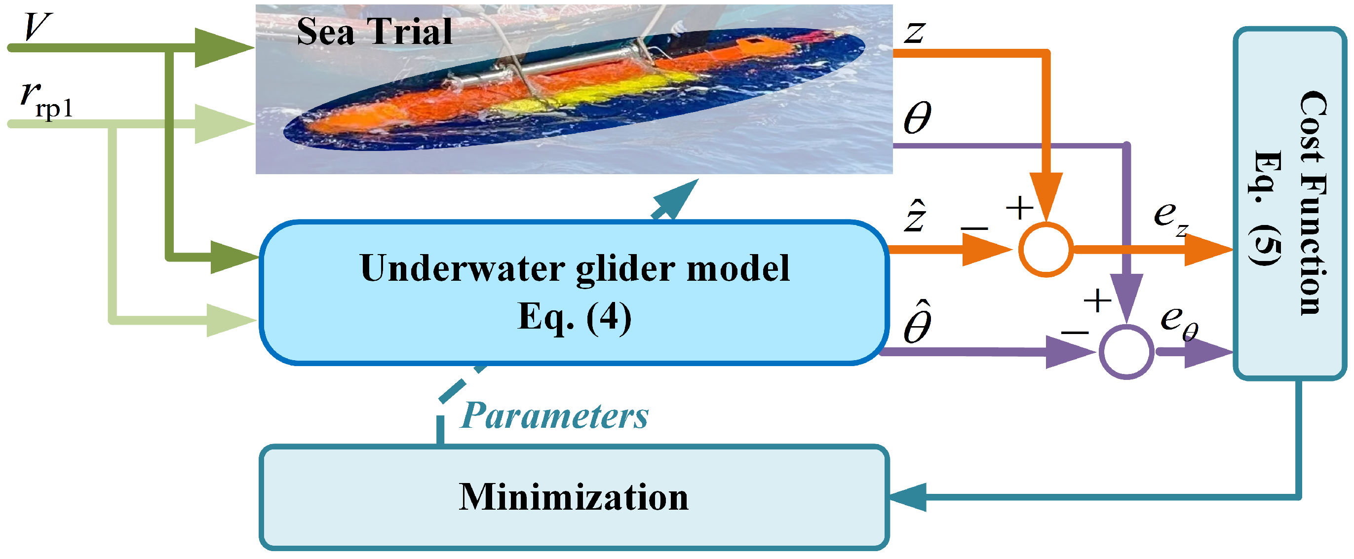
2.2. Parameter Identification

Based on the analysis in Section 2.1, altogether, eleven parameters of the dynamics model need to be identified, designated as $K_{\mathrm{h}}$, $K_{\mathrm{D}0}$, $K_{\mathrm{D}}$, $K_{\mathrm{L}0}$, $K_{\mathrm{L}}$, $K_{\mathrm{M}0}$, $K_{\mathrm{M}}$, $K_{\mathrm{q}}$, $J_{\mathrm{f}2}$, $M_{\mathrm{f}1}$, and $M_{\mathrm{f}3}$. The parameter identification toolbox in MATLAB 2024a is used, and the whole process is depicted in Figure 2. The cost function $F\left(t\right)$ is minimized as follows [39]:

$$F\left(t\right)=\sum _{i=0}^n{\left(z\left(t_i\right)-z_{\mathrm{s}}\left(t_i\right)\right)}^2+{\left(\theta \left(t_i\right)-{\theta }_{\mathrm{s}}\left(t_i\right)\right)}^2$$

(5)

where $z_{\mathrm{s}}$ and ${\theta }_{\mathrm{s}}$ are the dive depth and pitch angle in the sea trial, respectively.

Notably, the trust-region-reflective algorithm [40] is adopted in the parameter identification to optimize the selection process. The procedure for parameter identification is outlined in

Table 1. Parameter identification procedure.

Step	Procedure
Step 1	Utilize Simulink software (v. 24.2) to construct a nonlinear simulation model of the underwater glider.
Step 2	Import the sea trial data into the parameter identification toolbox in Simulink.
Step 3	Choose the parameters to be estimated and define the upper and lower bounds for each parameter.
Step 4	Configure the optimization and parallel computing settings.
Step 5	Execute the estimation process, iterating as needed to determine the desired parameters and optimize the cost function.
Step 6	Verify the accuracy of the model by assessing the simulated data against the estimated parameters. If significant discrepancies are found, iterate this process or adjust the model in Step 2, considering alternative identification methods if necessary.

:

2.3. Model Validation

Parameter identification is based on the data collected from the initial profile test of an underwater glider conducted in the South China Sea. For model validation, experimental data from profiles 28 to 39 are selected.

Table 2. Parameter identification results.

Parameters	Identification Results	Parameters	Identification Results
$K_{\mathrm{h}}$	−0.000257	$K_{\mathrm{M}}$	−124.60 kg/rad
$K_{\mathrm{D}0}$	6.33 $\mathrm{kg}/\mathrm{m}$	$K_{\mathrm{q}}$	−134.02 $\mathrm{kg}·\mathrm{s}/\mathrm{ra}{\mathrm{d}}^2$
$K_{\mathrm{D}}$	271.37 $\mathrm{kg}/\left(\mathrm{m}·\mathrm{ra}{\mathrm{d}}^2\right)$	$J_{\mathrm{f}2}$	−3.71 $\mathrm{kg}/{\mathrm{m}}^2$
$K_{\mathrm{L}0}$	5.85 $\mathrm{kg}/\mathrm{m}$	$M_{\mathrm{f}1}$	−59.16 $\mathrm{kg}$
$K_{\mathrm{L}}$	136.48 $\mathrm{kg}/\mathrm{m}$	$M_{\mathrm{f}3}$	114.37 $\mathrm{kg}$
$K_{\mathrm{M}0}$	2.10 $\mathrm{kg}$

presents the results of parameter identification.

Based on the data obtained from profiles 28 to 39 of the sea trial, the experimental results are compared with those predicted by the simplified model (Equation (4)) and the full model (Equation (1)). Figure 3 displays the comparison results in terms of dive depth and pitch angle. The simulation results from both models are highly consistent with the sea trial data. The root mean square error (RMSE) is employed to quantify the accuracy of the two models in representing the real underwater glider, expressed as follows [41]:

$$\mathrm{RMSE}=\sqrt{{\displaystyle \frac{1}{\mathrm{n}}}\sum _{i=1}^n{\left(y_i-{\hat{y}}_i\right)}^2}$$

(6)

where $y_i$ represents the true value and ${\widehat{y}}_i$ represents the observed value.

Table 3. RMSE for the dive depth and pitch angle with the full model and simplified model.

Parameters	Full Model	Simplified Model
z	33.8584	34.9584
$\theta$	0.9710	0.9730

presents the RMSE indices for the dive depth and pitch angle of both models. The results show the comparable accuracy of both models, indicating that they accurately capture the underwater glider’s behaviors.

2.4. Standard Forms

Based on Section 2.3, the parameter identification results are integrated into the underwater glider dynamics model (Equation (4)), leading to the following simplified form:

$$\left\{\begin{array}{cc}\hfill \dot{\mathit{\eta }}\left(t\right)& =\mathit{G}(\mathit{\eta }(t\left)\right)\mathit{\phi }\left(t\right)\hfill \\ \hfill \dot{\mathit{\phi }}\left(t\right)& =\mathit{M}{\mathit{F}}_1(\mathit{\eta }\left(t\right),\mathit{\phi }\left(t\right))+\mathit{M}{\mathit{F}}_2(\mathit{\eta }\left(t\right),\mathit{\phi }\left(t\right))\mathit{u}\left(t\right)\hfill \end{array}\right.$$

(7)

where the nonlinear vector function ${\mathit{F}}_1\left(t\right)\in {\mathbb{R}}^3$ is defined as follows:

$$\begin{array}{cc}\hfill {\mathit{F}}_1\left(t\right)& =\left[\begin{array}{c}{f}_1\left(t\right)\\ f_2\left(t\right)\\ f_3\left(t\right)\end{array}\right]\hfill \\ \hfill f_1\left(t\right)& =T_2\left(t\right)+0.0019cos\theta \left(t\right)·z\left(t\right)-2.06sin\theta \left(t\right)+158.53v_1\left(t\right)v_3\left(t\right)-0.21v_1\left(t\right)q\left(t\right)\hfill \\ \hfill f_2\left(t\right)& =-182.37v_3\left(t\right)q\left(t\right)+2.34sin\theta \left(t\right)+0.0025z\left(t\right)sin\theta \left(t\right)\hfill \\ \hfill & +L\left(t\right)sin\alpha \left(t\right)-D\left(t\right)cos\alpha \left(t\right)\hfill \\ \hfill f_3\left(t\right)& =8.85v_1\left(t\right)q\left(t\right)-2.34cos\theta \left(t\right)-0.0025z\left(t\right)cos\theta \left(t\right)\hfill \\ \hfill & -L\left(t\right)cos\alpha \left(t\right)+D\left(t\right)sin\alpha \left(t\right)\hfill \end{array}$$

The input-related matrix ${\mathit{F}}_2\left(t\right)\in {\mathbb{R}}^{3\times 2}$ is given by the following:

$${\mathit{F}}_2\left(t\right)=\left[\begin{array}{cc}-10.52cos\theta \left(t\right)-1.07v_1\left(t\right)q\left(t\right)& -147.15cos\theta \left(t\right)-15v_1\left(t\right)q\left(t\right)\\ -14.03sin\theta \left(t\right)& 0\\ 14.03cos\theta \left(t\right)& 0\end{array}\right]$$

The constant mass-inertia matrix $\mathit{M}\in {\mathbb{R}}^{3\times 3}$ is as follows:

$$\mathit{M}=\left[\begin{array}{ccc}0.048& 0& 0\\ 0& 0.11& 0\\ 0& 0& 0.0055\end{array}\right]$$

And the kinematic transformation matrix $\mathit{G}\left(t\right)\in {\mathbb{R}}^{2\times 3}$ is as follows:

$$\mathit{G}\left(t\right)=\left[\begin{array}{ccc}0& -sin\theta \left(t\right)& cos\theta \left(t\right)\\ 1& 0& 0\end{array}\right]$$

By defining ${\mathit{l}}_1\left(t\right)={\mathit{MF}}_{\mathbf{1}}(\mathit{\eta }\left(t\right),\mathit{\phi }\left(t\right))$, the dynamical model described in Equation (7) can be reformulated as follows:

$$\left\{\begin{array}{c}\dot{\mathit{\eta }}\left(t\right)=\mathit{G}(\mathit{\eta }\left(t\right))\mathit{\phi }\left(t\right)\hfill \\ \dot{\mathit{\phi }}\left(t\right)=\mathit{M}{\mathit{F}}_2(\mathit{\eta }\left(t\right),\mathit{\phi }\left(t\right))\mathit{u}\left(t\right)+{\mathit{l}}_1\left(t\right)\hfill \end{array}\right.$$

(8)

Then, the variable substitutions ${\mathit{x}}_1\left(t\right)=\mathit{\eta }\left(t\right)$ and ${\mathit{x}}_2\left(t\right)=\mathit{G}(\mathit{\eta }\left(t\right))\mathit{\phi }\left(t\right)$ are introduced to simplify the controller design process. Subsequently, Equation (8) can be further expressed as follows:

$$\left\{\begin{array}{c}{\dot{x}}_1\left(t\right)={\mathit{x}}_2\left(t\right)\hfill \\ {\dot{x}}_2\left(t\right)=G_2\left(x_1\left(t\right)\right)M{F}_2\left(x_1\left(t\right),x_2\left(t\right)\right)u\left(t\right)+G_2\left(x_1\left(t\right)\right)l\left(t\right)+\dot{\theta }{G}_1\left(x_1\left(t\right)\right)x_2\left(t\right)\hfill \end{array}\right.$$

(9)

where $G_1\left(x_1\left(t\right)\right)=\left[\begin{array}{ccc}0& sin\left(\theta \right(t\left)\right)& cos\left(\theta \right(t\left)\right)\\ 0& 0& 0\end{array}\right]$, and $G_2\left(x_1\left(t\right)\right)=\left[\begin{array}{ccc}0& -cos\left(\theta \right(t\left)\right)& sin\left(\theta \right(t\left)\right)\\ 1& 0& 0\end{array}\right]$.

Let $\mathit{F}\left(t\right)=G_2\left({\mathit{x}}_1\left(t\right)\right){\mathit{MF}}_{\mathbf{2}}\left({\mathit{x}}_1\left(t\right),{\mathit{x}}_2\left(t\right)\right)$, and ${\mathit{l}}_2\left(t\right)=G_2\left({\mathit{x}}_1\left(t\right)\right){\mathit{l}}_1\left(t\right)+\dot{\theta }{G}_1\left({\mathit{x}}_1\left(t\right)\right){\mathit{x}}_2\left(t\right)+\mathit{f}\left(t\right)$. Here, $\mathit{f}\left(t\right)$ represents the combined uncertainties of the unmodeled portion and the model’s time-varying components. Considering the changing disturbances at the inputs of the model represented as $d\left(t\right)$, the dynamical model can be written in the standard form as follows:

$$\left\{\begin{array}{c}{\dot{\mathit{x}}}_1\left(t\right)={\mathit{x}}_2\left(t\right)\hfill \\ {\dot{\mathit{x}}}_2\left(t\right)=\mathit{F}\left({\mathit{x}}_1\left(t\right),{\mathit{x}}_2\left(t\right)\right)(\mathit{u}\left(t\right)+\mathit{d}\left(t\right))+{\mathit{l}}_2\left(t\right)\hfill \end{array}\right.$$

(10)

Assumption 1

([42,43]). The uncertainty component of the model, ${\mathit{l}}_2\left(t\right)$, and the external perturbation, ${\mathit{d}}_1\left(t\right)$, are collectively treated as aggregate perturbations $\mathit{Ld}\left(t\right)$, where $\mathit{Ld}\left(t\right)$ is bounded and satisfies $\parallel \mathit{L}\mathit{d}\left(t\right)\parallel \le \mathit{L}{\mathit{d}}_{\mathrm{Max}}$. Under this assumption, Equation (10) can be reformulated into the following expression:

$$\left\{\begin{array}{c}{\dot{\mathit{x}}}_1\left(t\right)={\mathit{x}}_2\left(t\right)\hfill \\ {\dot{\mathit{x}}}_2\left(t\right)=\mathit{F}\left({\mathit{x}}_1\left(t\right),{\mathit{x}}_2\left(t\right)\right)\mathit{u}\left(t\right)+\mathit{L}\mathit{d}\left(t\right)\hfill \end{array}\right.$$

(11)

The main objective of this study is to develop a sliding mode controller based on a reinforcement learning framework. This control strategy is intended to effectively regulate the dive depth and pitch angle within a specified timeframe, while also improving resilience to external disturbances and uncertainties in the system model.

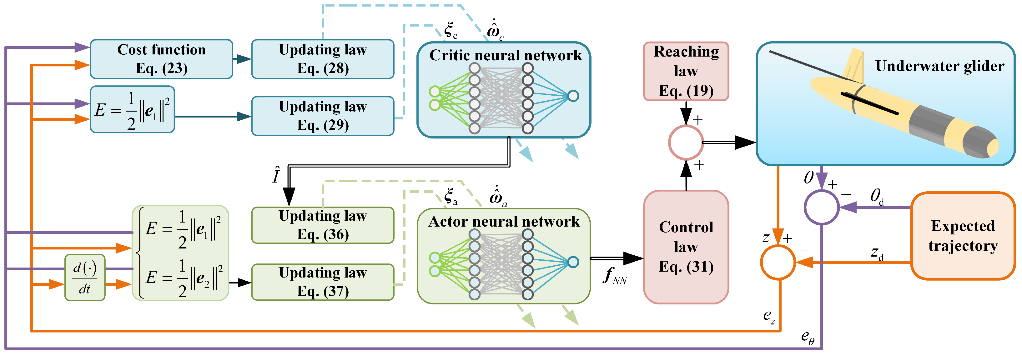
3. Controller Design

The schematic of controller design is shown in Figure 4.

3.1. Prior Knowledge

Lemma 1

([44]). Considering the nonlinear system $\dot{\mathit{x}}=f\left(\mathit{x}\left(t\right)\right)$, let $\mathit{x}\in {\mathit{R}}^n$, $x\left(0\right)=x_0$, where $f\left(\mathit{x}\right(t\left)\right)$ represents a nonlinear function. If Lyapunov function $V\left(x\right)$ exists, along with parameters $\alpha >0$, $\beta >0$, $0<p<1$, $q>1$, such that $\dot{V}\left(\mathit{x}\right)⩽-\left(\alpha V{\left(\mathit{x}\right)}^p+\beta V{\left(\mathit{x}\right)}^q\right)$, then, the system demonstrates stability within a fixed timeframe. The convergence time T satisfies the following:

$$T⩽{\displaystyle \frac{1}{\alpha (1-p)}}+{\displaystyle \frac{1}{\beta (q-1)}}$$

(12)

Lemma 2

(Young’s inequality, [45]). Suppose that $\mathit{a}$ and $\mathit{b}$ are vectors in ${\mathit{R}}^n$, and let p, q satisfy ${\displaystyle \frac{1}{p}+\frac{1}{q}=1}$; we can obtain the following:

$$\mathit{a}·\mathit{b}\le {\parallel a\parallel }_p{\parallel b\parallel }_q$$

(13)

where ${\parallel \mathit{a}\parallel }_p$ denotes the $L^p$-norm of the vector $\mathit{a}$. ${\parallel \mathit{b}\parallel }_q$ denotes the $L^q$-norm of the vector $\mathit{b}$.

3.2. Sliding Mode Controller Design

The desired trajectory is defined as ${\mathit{x}}_{1\mathrm{d}}={\left[\begin{array}{cc}{z}_{\mathrm{d}}\hfill & {\theta }_{\mathrm{d}}\hfill \end{array}\right]}^T$. The state error is subsequently determined as ${\mathbf{e}}_{1\mathrm{d}}={\mathit{x}}_1-{\mathit{x}}_{1\mathrm{d}}$, with the sliding mode surface denoted as $\mathit{S}={\left[\begin{array}{cc}{S}_1\hfill & S_2\hfill \end{array}\right]}^T$.

$$S_i={\dot{e}}_i+{\beta }_1{sig}^{{\psi }_i\left({\epsilon }_i\right)}\left(e_{1i}\right)+R_i\left(e_{1i}\right),i=1,2.$$

(14)

where ${\psi }_i\left({\epsilon }_1\right)=1+0.5{\epsilon }_1\left(1+sgn\left(\left|e_{1i}\right|-1\right)\right)$, and ${\beta }_1$ is the speed of convergence when the tracking error of the regulation system is away from the equilibrium point, with ${\beta }_1>0$. The expression of $R_i\left(e_{1i}\right)$ is presented as follows:

$$R_i\left(e_{1i}\right)=\left\{\begin{array}{cc}{\beta }_2{sig}^{{\varphi }_i\left({\epsilon }_2\right)}\left(e_{1i}\right),\hfill & \left|e_{1i}\right|⩾\delta \hfill \\ {\lambda }_1{e}_i+{\lambda }_2{sig}^{\gamma }\left(e_{1i}\right),\hfill & \left|e_{1i}\right|<\delta \hfill \end{array}\right.$$

(15)

where ${\lambda }_1={\beta }_2\left({\varphi }_i\left({\epsilon }_2\right)-\gamma \right){\delta }^{\delta \left({\epsilon }_2\right)-1}/(1-\gamma )$; ${\lambda }_2={\beta }_2\left({\varphi }_i\left({\epsilon }_2\right)-1\right){\delta }^{{\varphi }_1\left({\epsilon }_2\right)-\gamma }/(1-\gamma )$; ${\varphi }_i\left({\epsilon }_2\right)=1-0.5{\epsilon }_2\left(1-sgn\left(\left|e_{1i}\right|-1\right)\right)$; $\gamma$ determines the sliding mode surface, with $\gamma >0$; $\delta$ is a very small positive constant; and ${\beta }_2$ controls the rate of convergence of the tracking error near the equilibrium point, with ${\beta }_2>0$. The function ${sig}^a\left(x\right)$ is defined as ${sig}^a\left(x\right)={\left|x\right|}^{a}sgn\left(x\right)$.

Differentiating Equation (14) yields the following:

$${\dot{S}}_i={\ddot{e}}_{1i}+{\beta }_1{\psi }_i\left({\epsilon }_1\right){\left|e_{1i}\right|}^{{\psi }_i\left({\epsilon }_1\right)-1}{\dot{e}}_{1i}+{\dot{R}}_i\left(e_{1i}\right),i=1,2.$$

(16)

Let $\dot{\mathit{S}}=0$, the control law ${\mathit{u}}_1$ can be written as follows:

$${\mathit{u}}_1=-{\mathit{F}}^{-1}\left(\mathit{L}\mathit{d}\left(t\right)-{\ddot{\mathit{x}}}_{1\mathrm{d}}+{\beta }_1\psi \left({\epsilon }_1\right){\left|\mathit{e}\right|}^{\psi \left({\epsilon }_1\right)-1}\dot{\mathit{e}}+\dot{R}\left(\mathit{e}\right)\right)$$

(17)

To enhance the convergence speed and alleviate the chattering problems associated with sliding mode control, the following convergence law is proposed:

$${\dot{S}}_i=-K_{0}sgn\left(S_i\right)-K_1{sig}^{11+0.5{\alpha }_i\left(1+sgn\left(S_i-1-1\right)\right)}\left(S_i\right)-K_2{sig}^{1-0.5{\alpha }_2\left(1-sgn n\left(S_i\mid -1\right)\right)}\left(S_i\right),i=1,2$$

(18)

where $K_0$, $K_1$, and $K_2$ denote positive constants. The control rate for chattering suppression can be expressed as follows:

$${\mathit{u}}_2=-{\mathit{F}}^{-1}\dot{\mathit{S}}$$

(19)

where $\dot{\mathit{S}}={\left[\begin{array}{cc}{\dot{S}}_1\hfill & {\dot{S}}_2\hfill \end{array}\right]}^T$. In summary, the integrated control law can be written as follows:

$$\mathit{u}={\mathit{u}}_1+{\mathit{u}}_2$$

(20)

When the model is inaccurately constructed, the effectiveness of the control law outlined in Equation (20) may be compromised by the presence of a nonlinear term and an unknown disturbance, $\mathit{L}\mathit{d}\left(t\right)$, in the control law described in Equation (17).

To address this issue, we implement a critic–actor reinforcement learning strategy utilizing RBFNN. The critic network indirectly compensates for unknown disturbances by assessing the system’s performance metrics, which enables the dynamic adjustment of its weights. In contrast, the actor network directly generates error compensation signals. Its RBFNN architecture approximates the dynamic characteristics of disturbances through nonlinear mapping, integrating this estimation into the control law to actively mitigate the disturbances. Furthermore, we propose a real-time standard deviation updating strategy. The dynamic adjustment of the standard deviation optimizes the neural network’s local response capability, thereby enhancing its adaptability to the system’s nonlinear variations. This updating mechanism improves the network’s approximation accuracy and bolsters the control algorithm’s robustness against model uncertainties and external perturbations. Through online learning, the system continuously optimizes control performance, ensuring the precise management of underwater gliders in complex environments.

3.3. Critic Neural Network Design

This section presents the design of a critic neural network, which evaluates policy performance and optimizes the controller parameters. A method is proposed for updating the weights and standard deviations of the RBF neurons in real time, enhancing the network’s adaptability and robustness.

3.3.1. Weight Updates

Define the long-term cost function as follows [46,47]:

$$I\left(t\right)={\int }_0^{\infty }{e}_1^{-\frac{\tau -t}{\chi }}\phi \left(\tau \right)d\tau$$

(21)

where $\chi$ is a constant representing future costs and represents an immediate cost function, which can be expressed as follows:

$$\phi \left(t\right)={\mathit{e}}_1^T\mathit{D}{\mathit{e}}_1+{\mathit{u}}^T\mathit{R}\mathit{u}$$

(22)

where $\mathit{D}$ and $\mathit{R}$ are positive definite matrices.

Define $\mathit{I}={\omega }_c^{*T}{\sigma }_c\left({\mathit{e}}_1\right)+{\epsilon }_o$, and its estimate is $\hat{\mathit{I}}={{\hat{\omega }}_c}^T{\sigma }_c\left(e_1\right)$. Where ${\omega }_c^{*}$ and ${\hat{\omega }}_c$ are the true and estimated neural network weights, respectively, and ${\sigma }_c(·)$ takes the form of a Gaussian function as follows:

$${\sigma }_c\left(e\right)=exp\left({\displaystyle -\frac{{\sum }_{i=1}^r{\left(e_c-{\mu }_i\right)}^2}{2{\xi }_c^2}}\right)$$

(23)

Define the approximation error of the cost-to-go as follows:

$${\displaystyle \gamma \left(t\right)=\phi \left(t\right)-\frac{1}{\chi }\widehat{I}\left(t\right)+\dot{\widehat{I}}\left(t\right)}$$

(24)

Using gradient descent, the update law for the evaluation network is designed as follows [46]:

$${\dot{\hat{\omega }}}_c\left(t\right)=-{\displaystyle \frac{{\delta }_c}{2}}{\displaystyle \frac{\partial \left({\gamma }^2\left(t\right)\right)}{\partial {\omega }_c}}$$

(25)

where ${\delta }_c>0$ is the learning rate of the critic neural network. By substituting Equation (25) into Equation (24), we obtain the following:

$$\begin{array}{cc}\hfill {\dot{\widehat{\omega }}}_{\mathrm{c}}\left(t\right)& {\displaystyle =-\frac{{\delta }_c}{2}\frac{\partial \left({\gamma }^2\left(t\right)\right)}{\partial {\omega }_c}}\hfill \\ \hfill & {\displaystyle =-{\delta }_{\mathrm{c}}\gamma \left(t\right)\frac{\partial \left({\displaystyle \mathit{\phi }\left(t\right)-\frac{1}{\chi }\widehat{\mathit{I}}\left(t\right)+\widehat{\mathit{I}}\left(t\right)}\right)}{\partial {\omega }_c}}\hfill \\ \hfill & =-{\delta }_{\mathrm{c}}\gamma \left(t\right)\left({\displaystyle \frac{\partial \phi \left(t\right)}{\partial {\omega }_c}-\frac{1}{\chi }\frac{\partial \widehat{\mathit{I}}\left(t\right)}{\partial {\omega }_c}+\frac{\partial \dot{\mathit{I}}\left(t\right)}{\partial {\omega }_c}}\right)\hfill \\ \hfill & =-{\delta }_{\mathrm{c}}\left(\mathit{\phi }\left(t\right)+{\widehat{\omega }}_{\mathrm{c}}^T\left(t\right)\left({\displaystyle -\frac{1}{\chi }{\sigma }_{\mathrm{c}}\left(t\right)+\nabla {\sigma }_{\mathrm{c}}\left(t\right){\dot{e}}_1\left(t\right)}\right)\left({\displaystyle -\frac{1}{\chi }{\sigma }_c\left(t\right)+\nabla {\sigma }_{\mathrm{c}}\left(t\right){\dot{e}}_1\left(t\right)}\right)\right.\hfill \end{array}$$

(26)

Define ${\displaystyle \mathbf{\Theta }\left(t\right)=-\frac{1}{\chi }{\mathit{\sigma }}_{\mathrm{c}}\left(t\right)+{\dot{\mathit{\sigma }}}_{\mathrm{c}}\left(t\right){\dot{\mathit{e}}}_1\left(t\right)}$, and then, Equation (26) can be rewritten as follows:

$${\dot{\widehat{\omega }}}_c\left(t\right)=-{\delta }_c\left(\phi \left(t\right)+{\widehat{\omega }}_c^T\left(t\right)\mathbf{\Theta }\left(t\right)\right)\mathbf{\Theta }\left(t\right)$$

(27)

Define ${\mathit{\rho }}_c\left(t\right)=\left(\mathit{\phi }\left(t\right)+{\hat{\mathit{\omega }}}_{\mathrm{c}}^T\left(t\right)\mathbf{\Theta }\left(t\right)\right)\mathbf{\Theta }\left(t\right)$, and the updating law based on the projection method for the critic neural network is designed as follows:

$${\dot{\widehat{\omega }}}_c\left(t\right)=-{\delta }_c{\rho }_c\left(t\right)$$

(28)

3.3.2. Standard Deviation Update

Previous studies often emphasize weight updating strategies [46,47], but these approaches frequently fail to effectively address steady-state errors. To enhance the generalization capability of the neural network, this study introduces a gradient descent-based learning method specifically designed for the real-time adjustment of the standard deviation [48], optimizing the sensory field of the RBF networks.

$${\xi }_{\mathrm{c}}={\xi }_{\mathrm{c}}-{\eta }_c{\displaystyle \frac{\partial E}{\partial {\xi }_{\mathrm{c}}}}$$

(29)

where ${\eta }_c$ is the learning rate of the standard deviation update. Let ${\displaystyle E=\frac{1}{2}{∥e_1∥}^2}$, and ${\displaystyle \frac{\partial E}{\partial {\xi }_{\mathrm{c}}}}$ can be written as follows:

$$\begin{array}{cc}\hfill {\displaystyle \frac{\partial E}{\partial {\xi }_c}}& ={\displaystyle \frac{\partial E}{\partial {\mathit{e}}_1}}·{\displaystyle \frac{\partial e_1}{\partial {\sigma }_{\mathrm{c}}}}·{\displaystyle \frac{\partial {\sigma }_{\mathrm{c}}}{\partial {\xi }_c}}\hfill \\ \hfill & =-{\mathit{e}}_{\mathrm{c}}{\sigma }_{\mathrm{c}}\left(e\right)\left(-{\displaystyle \frac{{∥e_{\mathrm{c}}-{\mu }_i∥}^2}{{\xi }_c^3}}\right)\hfill \end{array}$$

(30)

Employing this method, the kernel width is adaptively expanded during phases of significant error to expedite the convergence of learning, while it is contracted during phases of minor error to enhance the accuracy of local approximation. This dynamically adjusted strategy not only effectively reduces modeling errors but also improves robustness against parameter uncertainty.

3.4. Actor Neural Network Design

3.4.1. Weighs’ Update

This section utilizes an actor neural network to approximate the aggregate disturbance in Equation (17). Specifically, ${\mathit{f}}_{NN}=\mathit{Ld}\left(t\right)$. The core of this approach lies in transforming the complex problem of disturbance estimation into a learned optimization process. By incorporating this into the control law, it can be formulated as follows:

$${\mathit{u}}_1=-{\mathit{F}}^{-1}\left({\mathit{f}}_{NN}-{\ddot{\mathit{x}}}_{1d}+{\beta }_1\psi \left({\epsilon }_1\right){\left|e\right|}^{\psi \left(s_1\right)-1}\dot{\mathit{e}}+\dot{R}\left(e\right)\right)$$

(31)

By using RBF neural networks, the following expression can be used to define ${\mathit{f}}_{NN}$:

$${\mathit{f}}_{NN}=\left[\begin{array}{c}{\widehat{\omega }}_{z1}{\sigma }_{z1}\left(e_z\right)+{\widehat{\omega }}_{z2}{\sigma }_{z2}\left({\dot{e}}_z\right)\hfill \\ {\widehat{\omega }}_{\theta 1}{\sigma }_{\theta 1}\left(e_{\theta }\right)+{\widehat{\omega }}_{\theta 2}{\sigma }_{\theta 2}\left({\dot{e}}_{\theta }\right)\hfill \end{array}\right]=\left[\begin{array}{c}{\widehat{\mathit{\omega }}}_z^T{\sigma }_z\hfill \\ {\widehat{\omega }}_{\theta }^T{\sigma }_{\theta }\hfill \end{array}\right]$$

(32)

The learning error of the ${\mathit{f}}_{NN}$ can be defined as follows:

$${\mu }_a=\Delta {\omega }_z^T{\sigma }_z+\Delta {\omega }_{\theta }^T{\sigma }_{\theta }$$

(33)

The actor neural network error is expressed as follows:

$$\begin{array}{cc}\hfill e_{\mathrm{a}}& ={\mu }_{\mathrm{a}}+k_{\mathrm{i}}\left(\widehat{I}\left(t\right)-I_{\mathrm{d}}\left(t\right)\right)\hfill \\ \hfill & ={\mu }_{\mathrm{a}}+k_{\mathrm{i}}\left({\omega }_{\mathrm{c}}^{*}{\sigma }_{\mathrm{c}}+{\epsilon }_{\mathrm{c}}-I_{\mathrm{d}}\left(t\right)\right)\hfill \end{array}$$

(34)

Define $\vartheta =tanh({\widehat{\omega }}_z^T{\sigma }_z+{\widehat{\omega }}_{\theta }^T{\sigma }_{\theta }+k_{\mathrm{i}}\widehat{I})$.

In the actor neural network, we utilize the following modified linear activation function:

$$R\left(\vartheta \right)=\left\{\begin{array}{cc}\vartheta \hfill & \mathrm{if}\vartheta >0\\ e^{\vartheta }-1\hfill & \mathrm{if}\vartheta \le 0\end{array}\right.$$

(35)

The renewal law for updating the parameters of the neural network is then expressed as:

$$\left\{\begin{array}{c}{\dot{\hat{\omega }}}_z=-{\delta }_{\mathrm{a}}R\left(\vartheta \right){\sigma }_z\hfill \\ {\dot{\hat{\omega }}}_{\theta }=-{\delta }_{\mathrm{a}}R\left(\vartheta \right){\sigma }_{\theta }\hfill \end{array}\right.$$

(36)

Define ${\rho }_z=R\left(\vartheta \right){\sigma }_z$ and ${\rho }_{\theta }=R\left(\vartheta \right){\sigma }_{\theta }$. The updating law of the actor neural network is designed as follows:

$${\dot{\hat{\omega }}}_a=-{\delta }_{\mathbf{a}}{\rho }_a,a=z,\theta$$

(37)

3.4.2. Standard Deviation Update

Inspired by the critic neural network’s update rule, an update rule is proposed for the standard deviations, which follows the gradient descent method, expressed as follows:

$${\xi }_{\mathrm{a}}={\xi }_{\mathrm{a}}-{\eta }_{\mathrm{a}}{e}_{\mathrm{a}}{\sigma }_{\mathrm{a}}\left(e\right)\left(-{\displaystyle \frac{{∥e_{\mathrm{a}}-{\mu }_i∥}^2}{{\xi }_{\mathrm{a}}^3}}\right),a=z,\theta$$

(38)

The stability analysis of the controller is shown in Appendix A.

4. Simulation Analysis

In this section, the proposed control law is applied to the dynamics model for the underwater glider to evaluate its practicality and effectiveness. The controller’s performance in rejecting disturbances and tracking trajectories is assessed through three distinct cases as follows:

1

Model uncertainty: This case examines the controller’s effectiveness in handling underwater glider dynamics with unmodeled components or time-varying hydrodynamic parameters, which introduce model uncertainty.

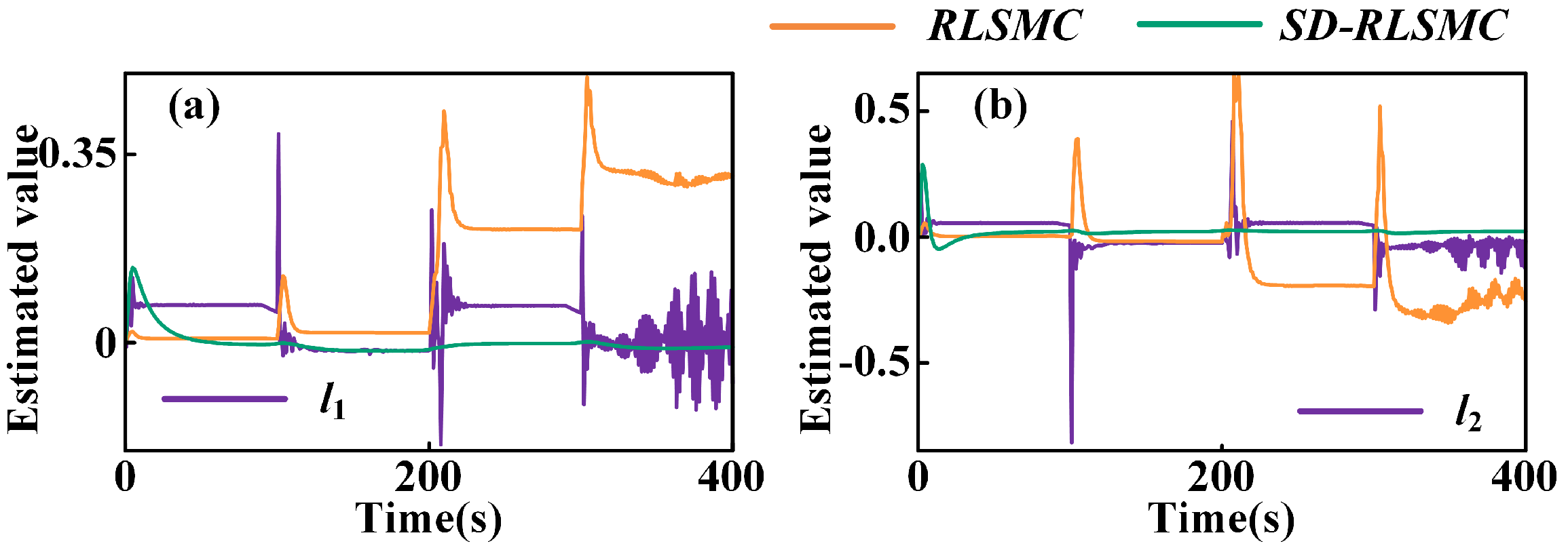
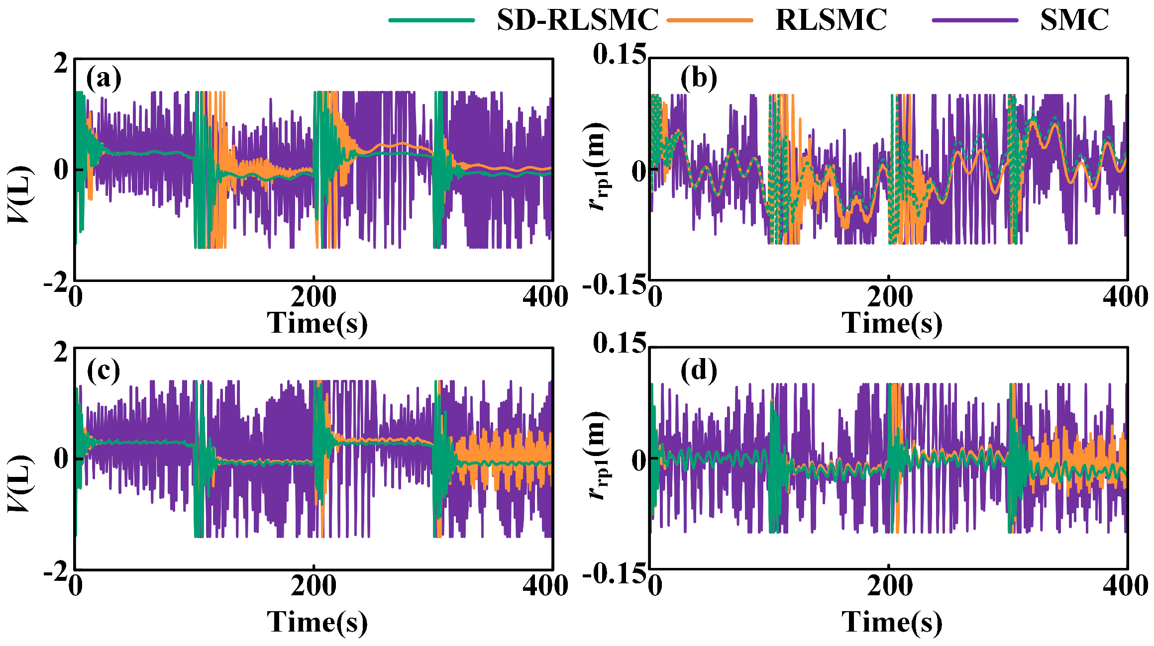
2

External disturbance suppression: The controller’s ability to suppress external disturbances is evaluated by applying two typical disturbances to the angular velocity q.

To evaluate the efficacy of various control strategies, simulations were executed utilizing the Simulink module in MATLAB 2024a. The methods assessed include the SMC, RLSMC, and SD-RLSMC algorithms. The simulations employed the ode4 (Runge-Kutta) solver with a fixed step size of 0.0005, spanning a total simulation duration of 400 s. Additionally, the neural network architecture adopted in this study is grounded in an actor–critic framework, employing RBF networks. Within this framework, all disturbances are consistently regarded as unmodeled dynamics, denoted by the term $f_{NN}=Ld\left(t\right)$, which is integrated into the control law to facilitate compensation. To ensure a fair comparison, the same initial conditions and relevant parameters are set for the simulation. The initial state of the underwater glider is defined as ${\left[\begin{array}{ccccc}z\hfill & \theta \hfill & q\hfill & v_1\hfill & v_3\hfill \end{array}\right]}^T={\left[\begin{array}{ccccc}0\hfill & 0\hfill & 0\hfill & 0\hfill & 0\hfill \end{array}\right]}^T$. The results of parameter identification are used to determine the hydrodynamic parameters, rotational inertia, and other relevant parameters, as shown in Table 2. The trajectories to be tracked can be expressed as follows:

$${\theta }_{\mathrm{d}}\left(\mathrm{rad}\right)=\left\{\begin{array}{cc}-0.32& 0\mathrm{s}\le t<100\mathrm{s}\\ 0.32& 100\mathrm{s}\le t<200\mathrm{s}\\ -0.32& 200\mathrm{s}\le t<300\mathrm{s}\\ 0.32& 300\mathrm{s}\le t<400\mathrm{s}\end{array}\right.$$

(39)

The z-direction trajectory of the underwater glider is indirectly controlled with its velocity. A velocity of $v_{1\mathrm{d}}=0.3\mathrm{m}/\mathrm{s}$ is assigned for horizontal movement. During descent, the velocity is set to $v_{3\mathrm{d}}=-0.03\mathrm{m}/\mathrm{s}$, and during ascent, it is set to $v_{3\mathrm{d}}=0.03\mathrm{m}/\mathrm{s}$. Consequently, the desired z-direction trajectory is represented as follows:

$$z_{\mathrm{d}}={\int }_0^t-v_{1\mathrm{d}}sin\left({\theta }_{\mathrm{d}}\right)+v_{3\mathrm{d}}cos\left({\theta }_{\mathrm{d}}\right)dt$$

(40)

The controller parameters are set in

Table 4. Controller parameter values.

Controller Composition	Variable
Critic NN	$\mathit{D}=0.9\left[\begin{array}{cc}1\hfill & \\ & 1\hfill \end{array}\right]$, $\mathit{R}=0.1\left[\begin{array}{cc}1\hfill & \\ & 1\hfill \end{array}\right]$,
	$\mu =\left[\begin{array}{ccc}-0.15:\hfill & 0.01:\hfill & 0.15\hfill \end{array}\right]$,
	$\psi =1$, ${\delta }_c=1$, ${\eta }_c=0.001$.
Active NN	$\mu =\left[\begin{array}{ccc}-0.15:\hfill & 0.01:\hfill & 0.15\hfill \end{array}\right]$,
	$\psi =1$, ${\delta }_{\mathrm{a}}=0.25$, $k_{\mathrm{I}}=1$, ${\eta }_a=0.001$.
SMC Controller	${\beta }_1=1$, ${\beta }_2=1$, ${\epsilon }_1=1$, ${\epsilon }_2=1$,
	$\gamma =10$, $\delta =0.01$, ${\alpha }_1=1$,
	${\alpha }_2=0.25$,
	$K_0=0.01$, $K_1=1$, $K_2=1$

.

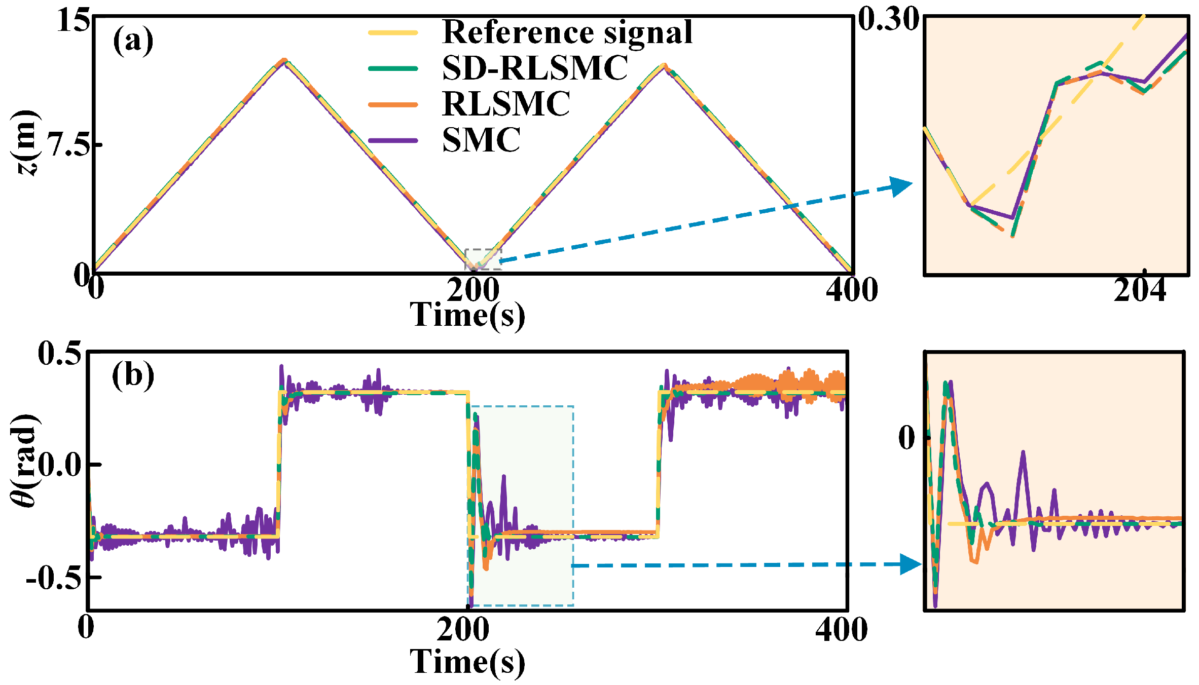
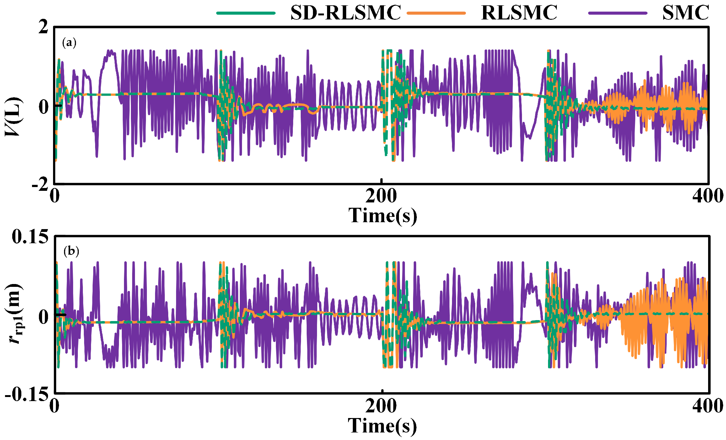
4.1. Case 1: Model Uncertainty

In the model parameter variation settings outlined in [20], parameter $K_{M0}$ was adjusted by up to 40% of its nominal value, while all other parameters experienced perturbations not exceeding 20%. To conduct a more thorough evaluation of the robustness of the control algorithm proposed in this study, we have increased the relative deviation of the model parameters to 25% and set them as varying with time. This enhanced configuration not only presents a more challenging scenario for testing the control algorithm under conditions of significant uncertainty but also more accurately reflects the dynamic variations encountered in real-world system operations. The general expression for the parameter variation is provided as follows:

$$K=\left(1+{\zeta }_{\mathrm{k}}25\%\right)K_0$$

(41)

where $0\le {\zeta }_{\mathrm{k}}\le 1$ characterizes the uncertainty of this parameter, and the frequency of change for ${\zeta }_{\mathrm{k}}$ is set to 0.2 Hz.

Figure 5 systematically compares the following three trajectory control strategies for underwater gliders: SD-RLSMC, RLSMC, and SMC. The tracking performance is depicted in terms of the dive depth (Figure 5a) and pitch angle (Figure 5b). The findings suggest that all methods effectively track the depth trajectory; however, both SD-RLSMC and RLSMC exhibit larger errors around $t=200$ s compared to SMC. Nonetheless, the quantitative analysis presented in

Table 5. RMSE and overshoot of the diving depth and pitch angle.

Parameter	Controllers	RMSE	Overshoot
z	SMC	0.0228	0.21%
	RLSMC	0.0285	0.02%
	SD-RLSMC	0.0154	0.01%
$\theta$	SMC	0.0659	36.13%
	RLSMC	0.0514	30.74%
	SD-RLSMC	0.0430	9.77%

indicates that SD-RLSMC achieves the lowest RMSE in dive depth at 0.0154, surpassing RLSMC (0.0285) and SMC (0.0228). Notably, the overshoot of SD-RLSMC is merely 0.01%, considerably lower than that of the other strategies. Similarly, for pitch angle control, SD-RLSMC attains an RMSE of 0.0430 with an overshoot of 9.77%, demonstrating superior accuracy and stability under dynamic conditions.

The controller outputs for the tracking of the intended trajectory are illustrated in Figure 6. It is evident that the actuator demonstrates significant vibrations when SMC is implemented. In contrast, the RLSMC and SD-RLSMC strategies significantly reduce vibrations, with SD-RLSMC exhibiting the lowest levels of vibration. This implies that SD-RLSMC is highly effective in reducing actuator strain and is distinguished by its exceptional energy efficiency. To quantitatively evaluate the control effort, the power associated with the control signals $dV$ and $r_{p1}$ is computed. The control power is calculated using the following expression:

$$\mathrm{Power}={\displaystyle \frac{1}{N}}\sum u_i^2$$

(42)

As shown in the

Table 6. Controller power.

Parameter	Controllers	Power
$dV$	SMC	0.7841
	RLSMC	0.1500
	SD-RLSMC	0.1573
$r_{rp1}$	SMC	0.0036
	RLSMC	0.0011
	SD-RLSMC	0.0006

, the SMC strategy exhibits a significantly higher control effort in both the $dV$ and $r_{p1}$ control signals compared to the other two strategies. Notably, the control effort of SD-RLSMC is slightly lower than that of RLSMC, demonstrating the effectiveness of SD-RLSMC in reducing actuator energy consumption.

Figure 7 presents the outcomes of the neural network estimations of the aggregated disturbances within the simplified model, employing both the RLSMC and SD-RLSMC methodologies. The figure demonstrates that the SD-RLSMC algorithm yields a comparatively more precise estimation of disturbances, whereas the RLSMC algorithm exhibits substantial deviation as simulation time advances.

4.2. Case 2: External Disturbance Suppression

Ocean currents and winds are integral components of the marine environment, with disturbances induced by these currents exerting a substantial influence on the movement of underwater vehicles. The velocity and direction of ocean currents exhibit significant variability across different geographical regions and seasonal periods, with surface currents generally demonstrating greater intensity compared to deep-sea currents. Despite this, there is presently no model that can precisely capture the intricate behavior of ocean currents. To address the impact of external currents on the dynamics of gliders, Zhou et al. [49] and Zou et al. [20] propose the introduction of perturbation signals into the q velocity component, as follows:

$$q_{\mathrm{dis}1}=0.33sin\left(0.1t\right)+0.25cos\left(0.02t\right)+0.3sin\left(0.1t\right)cos\left(0.2t\right)$$

(43)

$$q_{\mathrm{dis}2}=0.02sin\left(0.9t\right)+0.03cos\left(1.1t\right)-0.05sin\left(0.8t\right)$$

(44)

From these two equations, it becomes apparent that the perturbation signifies a large-amplitude, slowly varying the signal employed to characterize surface wave conditions. Conversely, the second perturbation is indicative of a small-amplitude, rapidly fluctuating signal, which represents the impact of underwater currents.

Figure 8a,b illustrates the trajectory tracking performance of the three algorithms when subjected to large-amplitude, slow time-varying disturbance signal, thereby offering a visual depiction of each algorithm’s control efficacy. The RMSE values presented in

Table 7. RMSE and overshoot of the diving depth and pitch angle.

Parameter	Controllers	${\mathit{q}}_{\mathbf{dis}1}$		${\mathit{q}}_{\mathbf{dis}2}$
		RMSE	Overshoot	RMSE	Overshoot
z	SMC	0.0278	0.12%	0.284	0.03%
	RLSMC	0.1480	0.03%	0.0401	0.02%
	SD-RLSMC	0.0159	0.05%	0.0145	0.02%
$\theta$	SMC	0.1340	113.64%	0.1082	89.82%
	RLSMC	0.1161	63.04%	0.0591	31.79%
	SD-RLSMC	0.0722	20.39%	0.0304	16.21%

quantitatively substantiate these visual observations. In terms of dive depth, while the tracking performance of the SD-RLSMC algorithm is marginally inferior to that of the RLSMC algorithm, its RMSE value is 0.0159, which is significantly lower than the RMSE values of RLSMC (0.1480) and SMC (0.0278). Regarding pitch angle tracking, as depicted in Figure 8b, the SMC algorithm demonstrates a pronounced oscillation phenomenon, whereas the RLSMC algorithm exhibits fluctuations upon each adjustment of the pitch angle, achieving stability only after a delay while still displaying steady-state errors. Conversely, the SD-RLSMC algorithm demonstrates minimal oscillation and negligible steady-state error. Moreover, Table 7 indicates that the RMSE for SD-RLSMC is 0.0722, substantially lower than that of RLSMC (0.1161) and SMC (0.1340), thereby underscoring the superior tracking stability of the SD-RLSMC algorithm in these two metrics. Furthermore, the overshoot data presented in Table 7 corroborate this observation. The overshoot in pitch angle tracking for the SD-RLSMC method is markedly lower compared to the other two methods, indicating that the algorithm provides enhanced stability and accuracy during the response process by effectively mitigating overreactions and oscillations. This advantage likely arises from the standard deviation adaptive feature incorporated into the SD-RLSMC algorithm, which facilitates dynamic adjustments to the control strategy in response to disturbances, thereby significantly reducing tracking errors.

Figure 8c,d provides additional evidence of the trajectory tracking performance of the three algorithms when subjected to small-amplitude, rapidly varying signal perturbations, thereby corroborating the previous findings. In the context of dive depth and pitch angle tracking, the SD-RLSMC algorithm consistently outperforms the RLSMC and significantly exceeds the performance of the SMC. Notably, under these conditions, SD-RLSMC does not display any discernible steady-state error, further affirming its robust control capabilities. The overshoot calculations presented in Table 7 substantiate the continued superiority of SD-RLSMC in pitch angle tracking, underscoring the algorithm’s enhanced adaptability in managing small-amplitude, rapidly varying signal perturbations.

Figure 9 illustrates the controller outputs used to track the target trajectory. It is evident that significant vibrations occur when using SMC. In contrast, both RLSMC and SD-RLSMC strategies effectively reduce vibration levels, with SD-RLSMC exhibiting the lowest vibration. To quantitatively assess the control effort, we calculated the power of the control signals for the three algorithms under two perturbation scenarios, with the results presented in

Table 8. Controller power.

Parameter	Controllers	Power
		${\mathit{q}}_{\mathit{dis}\mathbf{1}}$	${\mathit{q}}_{\mathit{dis}\mathbf{2}}$
$dV$	SMC	0.9582	0.9582
	RLSMC	0.3234	0.1852
	SD-RLSMC	0.2038	0.1346
$r_{p1}$	SMC	0.0044	0.0044
	RLSMC	0.0021	0.0008
	SD-RLSMC	0.0016	0.0006

. The SD-RLSMC strategy demonstrates significantly lower control effort, in terms of both dV and rp1 power, compared to the other two strategies. Notably, the control effort of SD-RLSMC is slightly lower than that of RLSMC, indicating its effectiveness in reducing actuator energy consumption.

Table 9. Comparison of performance for underwater glider control algorithms.

Reference	Performance Effect
Wang et al., 2025 [23]	Average integral absolute error: 0.29
Zou et al., 2024 [20]	Trajectory tracking error between ${10}^{-6}$ and ${10}^{-4}$
Juan et al., 2024 [22]	Average control errors in velocities along u, v, and w directions: 0.5195 ± 0.5452, 0.4703 ± 0.5859, and 0.2149 ± 0.3041
Lei et al., 2024 [24]	Pitch angle steady-state error less than $0.1$ rad
This paper	For various disturbances: Z-direction RMSE between 0.0145 and 0.0159; RMSE in other directions between 0.003 and 0.007

presents performance metrics from the literature for an initial comparison. The algorithm in this paper is similar to existing control methods in structure, interference immunity, and system modeling, with no significant drawbacks. Although the literature uses different evaluation metrics, this study’s control performance metrics are comparably high, indicating the proposed method’s effectiveness and potential benefits.

5. Conclusions and Prospects

This study presents the implementation of a finite-time sliding mode trajectory tracking control strategy for underwater gliders, known as SD-RLSMC, which incorporates the radial basis function neural network reinforcement learning method. The identification of hydrodynamic and pertinent parameters is achieved through data collected during sea trials, facilitating the development of the precise and appropriate dynamic model for controller formulation. The reinforcement learning framework incorporates a critic neural network for strategy evaluation and optimization and the actor neural networks for addressing model uncertainties, the external environment, and actuator disturbances. These estimations are integrated as feedback terms within the sliding mode control framework. To improve the generalization capability and robustness of the control system, a mechanism for updating the weights and standard deviations in both critic and actor Neural Networks is proposed. The simulation results illustrate that the control strategy exhibits consistent and reliable performance across diverse conditions, encompassing unmodeled influences and external disturbances.

While the control method proposed in this paper presents several advantages, it also exhibits certain limitations. Firstly, when addressing large-amplitude, slow time-varying disturbances, the controller partially mitigates the steady-state error; however, control oscillations remain discernible, and jittering behavior is evident during the attitude adjustment phase. Secondly, the integration of multiple components, including sliding mode control and radial basis function neural networks, complicates the parameter tuning process, thereby increasing the difficulty of algorithm debugging in practical engineering applications.

Future research endeavors will focus on simplifying the control strategy, refining the algorithms governing weights and standard deviation updates, and crafting a trajectory tracking control algorithm tailored to underwater gliders navigating three-dimensional space. Furthermore, the efficacy of the proposed SD-RLSMC scheme will be assessed through experimentation on an actual underwater glider system to verify its practical utility.

References

1. Tian, B.; Guo, J.; Song, Y.; Zhou, Y.; Xu, Z.; Wang, L. Research progress and prospects of gliding robots applied in ocean observation. J. Ocean Eng. Mar. Energy 2023, 9, 113–124. [Google Scholar] [CrossRef]
2. Yuan, S.; Li, Y.; Bao, F.; Xu, H.; Yang, Y.; Yan, Q.; Zhong, S.; Yin, H.; Xu, J.; Huang, Z.; et al. Marine environmental monitoring with unmanned vehicle platforms: Present applications and future prospects. Sci. Total Environ. 2023, 858, 159741. [Google Scholar] [CrossRef] [PubMed]
3. Jiang, Z.; Wu, H.; Wu, Q.; Yang, Y.; Tan, L.; Yan, S. Control parameter optimization based trajectory design of underwater gliders executing underwater fixed-point exploration missions. Ocean Eng. 2023, 279, 114127. [Google Scholar] [CrossRef]
4. Joshi, B.; Xanthidis, M.; Roznere, M.; Burgdorfer, N.J.; Mordohai, P.; Li, A.Q.; Rekleitis, I. Underwater exploration and mapping. In Proceedings of the 2022 IEEE/OES Autonomous Underwater Vehicles Symposium (AUV), Singapore, 19–21 September 2022; pp. 1–7. [Google Scholar]
5. Alexandris, C.; Papageorgas, P.; Piromalis, D. Positioning Systems for Unmanned Underwater Vehicles: A Comprehensive Review. Appl. Sci. 2024, 14, 9671. [Google Scholar] [CrossRef]
6. Liang, Y.; Wang, Y.; Zhang, L.; Wang, Y.; Yang, M.; Niu, W.; Yang, S. Conceptual design and analysis of a two-stage underwater glider for ultra-long voyage. Appl. Ocean Res. 2023, 138, 103639. [Google Scholar] [CrossRef]
7. Yang, H.; Mahmoudian, N. Gliding in extreme waters: Dynamic Modeling and Nonlinear Control of an Agile Underwater Glider. arXi 2024, arXiv:2402.06055. [Google Scholar] [CrossRef]
8. Liu, Y.; Liu, J.; Pan, G.; Huang, Q.; Guo, L. Vibration Analysis and Isolator Component Design of the Power System in an Autonomous Underwater Glider. Int. J. Acoust. Vib. 2022, 27, 112–121. [Google Scholar] [CrossRef]
9. Leonard, N.E.; Graver, J.G. Model-based feedback control of autonomous underwater gliders. IEEE J. Ocean. Eng. 2001, 26, 633–645. [Google Scholar] [CrossRef]
10. Liu, Y.; Su, Z.; Luan, X.; Song, D.; Han, L. Motion analysis and fuzzy-PID control algorithm designing for the pitch angle of an underwater glider. J. Math. Comput. Sci. 2017, 17, 133–147. [Google Scholar] [CrossRef]
11. Landau, I.D.; Lozano, R.; M’Saad, M.; Karimi, A. Adaptive Control: Algorithms, Analysis and Applications; Springer Science & Business Media: Berlin/Heidelberg, Germany, 2011. [Google Scholar]
12. Wan, L.; Zhang, D.; Sun, Y.; Qin, H.; Cao, Y.; Chen, G. Fast fixed-time vertical plane motion control of autonomous underwater gliders in shallow water. J. Frankl. Inst. 2022, 359, 10483–10509. [Google Scholar] [CrossRef]
13. Sang, H.; Zhou, Y.; Sun, X.; Yang, S. Heading tracking control with an adaptive hybrid control for under actuated underwater glider. ISA Trans. 2018, 80, 554–563. [Google Scholar] [CrossRef] [PubMed]
14. Nguyen, N.D.; Choi, H.s.; Jin, H.S.; Huang, J.; Lee, J.H. Robust Adaptive Depth Control of hybrid underwater glider in vertical plane. Adv. Technol. Innov. 2020, 5, 135–146. [Google Scholar] [CrossRef]
15. García-Valdovinos, L.G.; Salgado-Jiménez, T.; Bandala-Sánchez, M.; Nava-Balanzar, L.; Hernández-Alvarado, R.; Cruz-Ledesma, J.A. Modelling, design and robust control of a remotely operated underwater vehicle. Int. J. Adv. Robot. Syst. 2014, 11, 1. [Google Scholar] [CrossRef]
16. Ding, W.; Wei, D.; Diao, Y.; Yang, C.; Zhang, X.; Zhang, X.; Huang, H. Research on trajectory tracking control of ocean unmanned aerial vehicles based on disturbance observer and nonlinear sliding mode. Ocean Eng. 2024, 293, 116682. [Google Scholar] [CrossRef]
17. Zeng, Z.; Lyu, C.; Bi, Y.; Jin, Y.; Lu, D.; Lian, L. Review of hybrid aerial underwater vehicle: Cross-domain mobility and transitions control. Ocean Eng. 2022, 248, 110840. [Google Scholar] [CrossRef]
18. Zhang, X.; Zhou, H.; Fu, J.; Wen, H.; Yao, B.; Lian, L. Adaptive integral terminal sliding mode based trajectory tracking control of underwater glider. Ocean Eng. 2023, 269, 113436. [Google Scholar] [CrossRef]
19. Zhou, H.; Xu, H.; Cao, J.; Fu, J.; Mao, Z.; Zeng, Z.; Yao, B.; Lian, L. Robust adaptive control of underwater glider for bottom sitting-oriented soft landing. Ocean Eng. 2024, 293, 116725. [Google Scholar] [CrossRef]
20. Zou, H.; Zhang, G.; Hao, J. Nonsingular fast terminal sliding mode tracking control for underwater glider with actuator physical constraints. ISA Trans. 2024, 146, 249–262. [Google Scholar] [CrossRef]
21. Roy, R.G.; Ghoshal, D. A novel adaptive second-order sliding mode controller for autonomous underwater vehicles. Adapt. Behav. 2021, 29, 39–54. [Google Scholar] [CrossRef]
22. Juan, R.; Wang, T.; Liu, S.; Zhou, Y.; Ma, W.; Niu, W.; Gao, Z. High-precision motion control of underwater gliders based on reinforcement learning. Ocean Eng. 2024, 310, 118603. [Google Scholar] [CrossRef]
23. Wang, J.; Chen, Y.; Gao, J.; Min, B.; Pan, G. Adaptive fault tolerant control of unmanned underwater glider with predefined-time stability. J. Frankl. Inst. 2025, 362, 107364. [Google Scholar] [CrossRef]
24. Lei, L.; Gang, Y.; Jing, G. Physics-guided neural network for underwater glider flight modeling. Appl. Ocean Res. 2022, 121, 103082. [Google Scholar] [CrossRef]
25. Jeong, S.k.; Choi, H.S.; Ji, D.H.; Kim, J.Y.; Hong, S.M.; Cho, H.J. A study on an accurate underwater location of hybrid underwater gliders using machine learning. J. Mar. Sci. Technol. 2020, 28, 7. [Google Scholar]
26. Gao, J.; Min, B.; Chen, Y.; Jing, A.; Wang, J.; Pan, G. Compound learning based event-triggered adaptive attitude control for underwater gliders with actuator saturation and faults. Ocean Eng. 2023, 280, 114651. [Google Scholar] [CrossRef]
27. Emami, S.A.; Castaldi, P.; Banazadeh, A. Neural network-based flight control systems: Present and future. Annu. Rev. Control 2022, 53, 97–137. [Google Scholar] [CrossRef]
28. Su, Z.q.; Zhou, M.; Han, F.f.; Zhu, Y.w.; Song, D.l.; Guo, T.t. Attitude control of underwater glider combined reinforcement learning with active disturbance rejection control. J. Mar. Sci. Technol. 2019, 24, 686–704. [Google Scholar] [CrossRef]
29. Zang, W.; Yao, P.; Song, D. Standoff tracking control of underwater glider to moving target. Appl. Math. Model. 2022, 102, 1–20. [Google Scholar] [CrossRef]
30. Mirza, J.; Kanwal, F.; Salaria, U.A.; Ghafoor, S.; Aziz, I.; Atieh, A.; Almogren, A.; Haq, A.U.; Kanwal, B. Underwater temperature and pressure monitoring for deep-sea SCUBA divers using optical techniques. Front. Phys. 2024, 12, 1417293. [Google Scholar] [CrossRef]
31. Mirza, J.; Atieh, A.; Kanwal, B.; Ghafoor, S.; Almogren, A.; Kanwal, F.; Aziz, I. Relay aided UWOC-SMF-FSO based hybrid link for underwater wireless optical sensor network. Opt. Fiber Technol. 2025, 89, 104045. [Google Scholar] [CrossRef]
32. Wang, Y.; Thanyamanta, W.; Bose, N. Cooperation and compressed data exchange between multiple gliders used to map oil spills in the ocean. Appl. Ocean Res. 2022, 118, 102999. [Google Scholar] [CrossRef]
33. Shi, Y.; Dong, H.; He, C.R.; Chen, Y.; Song, Z. Mixed Vehicle Platoon Forming: A Multi-Agent Reinforcement Learning Approach. IEEE Internet Things J. 2025. [Google Scholar]
34. Fossen, T.I. Marine Control Systems—Guidance: Navigation, and Control of Ships, Rigs and Underwater Vehicles; Marine Cybernetics, Trondheim, Norway, Org. Number NO 985 195 005 MVA; Springer: Berlin/Heidelberg, Germany, 2002; ISBN 82-92356-00-2. Available online: www.marinecybernetics.com (accessed on 1 April 2025).
35. Wang, G.; Yang, Y.; Wang, S. Adaptive digital disturbance rejection controller design for underwater thermal vehicles. J. Mar. Sci. Eng. 2021, 9, 406. [Google Scholar] [CrossRef]
36. Yang, Y.; Liu, Y.; Wang, Y.; Zhang, H.; Zhang, L. Dynamic modeling and motion control strategy for deep-sea hybrid-driven underwater gliders considering hull deformation and seawater density variation. Ocean Eng. 2017, 143, 66–78. [Google Scholar] [CrossRef]
37. Hussain, N.A.A.; Arshad, M.R.; Mohd-Mokhtar, R. Underwater glider modelling and analysis for net buoyancy, depth and pitch angle control. Ocean Eng. 2011, 38, 1782–1791. [Google Scholar]
38. Liang, Y.; Zhang, L.; Yang, M.; Wang, Y.; Niu, W.; Yang, S. Dynamic behavior analysis and bio-inspired improvement of underwater glider with passive buoyancy compensation gas. Ocean Eng. 2022, 257, 111644. [Google Scholar]
39. Miniguano, H.; Barrado, A.; Lázaro, A.; Zumel, P.; Fernández, C. General parameter identification procedure and comparative study of Li-Ion battery models. IEEE Trans. Veh. Technol. 2019, 69, 235–245. [Google Scholar] [CrossRef]
40. Tekin, M.; Karamangil, M.I. Development of dual polarization battery model with high accuracy for a lithium-ion battery cell under dynamic driving cycle conditions. Heliyon 2024, 10, e28454. [Google Scholar] [CrossRef]
41. Hodson, T.O. Root mean square error (RMSE) or mean absolute error (MAE): When to use them or not. Geosci. Model Dev. Discuss. 2022, 2022, 5481–5487. [Google Scholar] [CrossRef]
42. Lee, T.H.; Harris, C.J. Adaptive Neural Network Control of Robotic Manipulators; World Scientific: Singapore, 1998; Volume 19. [Google Scholar]
43. Guo, Q.; Li, X.; Zuo, Z.; Shi, Y.; Jiang, D. Quasi-synchronization control of multiple electrohydraulic actuators with load disturbance and uncertain parameters. IEEE/ASME Trans. Mechatronics 2020, 26, 2048–2058. [Google Scholar] [CrossRef]
44. Jiang, B.; Hu, Q.; Friswell, M.I. Fixed-time attitude control for rigid spacecraft with actuator saturation and faults. IEEE Trans. Control Syst. Technol. 2016, 24, 1892–1898. [Google Scholar] [CrossRef]
45. Saeki, S. The Lp-conjecture and Young’s inequality. Ill. J. Math. 1990, 34, 614–627. [Google Scholar]
46. Ouyang, Y.; He, W.; Li, X. Reinforcement learning control of a single-link flexible robotic manipulator. IET Control Theory Appl. 2017, 11, 1426–1433. [Google Scholar] [CrossRef]
47. Cao, S.; Sun, L.; Jiang, J.; Zuo, Z. Reinforcement learning-based fixed-time trajectory tracking control for uncertain robotic manipulators with input saturation. IEEE Trans. Neural Netw. Learn. Syst. 2021, 34, 4584–4595. [Google Scholar] [CrossRef] [PubMed]
48. Panda, S.; Panda, G. On the development and performance evaluation of improved radial basis function neural networks. IEEE Trans. Syst. Man Cybern. Syst. 2021, 52, 3873–3884. [Google Scholar] [CrossRef]
49. Zhou, H.; Wei, Z.; Zeng, Z.; Yu, C.; Yao, B.; Lian, L. Adaptive robust sliding mode control of autonomous underwater glider with input constraints for persistent virtual mooring. Appl. Ocean Res. 2020, 95, 102027. [Google Scholar] [CrossRef]
50. Steele, J.M. The Cauchy-Schwarz Master Class: An Introduction to the Art of Mathematical Inequalities; Cambridge University Press: Cambridge, UK, 2004. [Google Scholar]
Figure 1. Schematic diagram of the underwater glider.
Jmse 13 00884 g001
Figure 2. Schematic diagram of parameter identification.
Jmse 13 00884 g002
Figure 3. Comparison between the full model simulation, simplified model simulation, and sea trial data. (a) Diving depth, (b) pitch angle.
Jmse 13 00884 g003
Figure 4. Schematic of controller design.
Jmse 13 00884 g004
Figure 5. Trajectory tracking of an underwater glider utilizing SD-RLSMC, RLSMC, and SMC. (a) Dive depth. (b) Pitch angle.
Jmse 13 00884 g005
Figure 6. Actuator outputs of an underwater glider utilizing SD-RLSMC, RLSMC, and SMC. (a) Buoyancy adjustment. (b) Position of the attitude adjustment unit.
Jmse 13 00884 g006
Figure 7. Estimation results of actor NN on unmodel parts in SD-RLSMC and RLSM. (a) The estimation results for l 1 . (b) The estimation results for l 2 .
Jmse 13 00884 g007
Figure 8. Performance of SD-RLSMC, RLSMC, and SMC for depth and pitch angle tracking. (a) q dis 1 for depth, (b) q dis 1 for pitch angle, (c) q dis 2 for depth, (d) q dis 2 for pitch angle.
Jmse 13 00884 g008
Figure 9. Buoyancy regulation and positions of the attitude adjustment units with SD-RLSMC, RLSMC, and SMC. (a) q dis 1 for V, (b) q dis 1 for r r p 1 , (c) q dis 2 for V, (d) q dis 2 for r r p 1 .
Jmse 13 00884 g009