
A Trajectory Tracking Control Method for 6 DoF UUV Based on Event Triggering Mechanism


Abstract
1. Introduction
- In real environments, the UUV usually uses propellers. The rotation of propellers produces reaction torque to affect the roll angle of the UUV, which leads to the roll motion of the UUV. However, the above methods focus on considering the impact of introducing external environmental disturbances to the trajectory tracking of UUVs. The above methods fail to consider the influence of propellers comprehensively. Therefore, we should design the trajectory tracking control method of UUVs under the influence of reaction torque.
- When performing complex trajectory tracking, the roll angle of UUV impacts trajectory tracking significantly. However, the above methods often use the 5 DoF UUV. In addition, the communication resource and computational resource for UUVs are limited. Hence, the above methods fail to establish the 6 DoF model of UUVs and optimize the resource consumption of UUVs.
- Problem: A scenario for the motion control of 6 DOF UUV under the reaction torque of propeller is established. According to the kinematic model and dynamic model of the UUV, this paper designs the kinematic model and dynamic model of 6-DOF UUVs under the influence of reaction torque, which contributes to the design of corresponding controllers.
- Method: A dual loop integral sliding mode controller is designed to achieve the trajectory tracking control of 6-DOF UUVs. This paper realizes error stabilization through the integral sliding surfaces of position loop controller and speed loop controller. Then, an event triggering mechanism based on relative threshold is proposed to reduce the output frequency of control signals. In addition, the positive lower bound method is used to demonstrate the feasibility of the event triggering mechanism, and the Lyapunov theorem is used to prove the stability of EDLISMC.
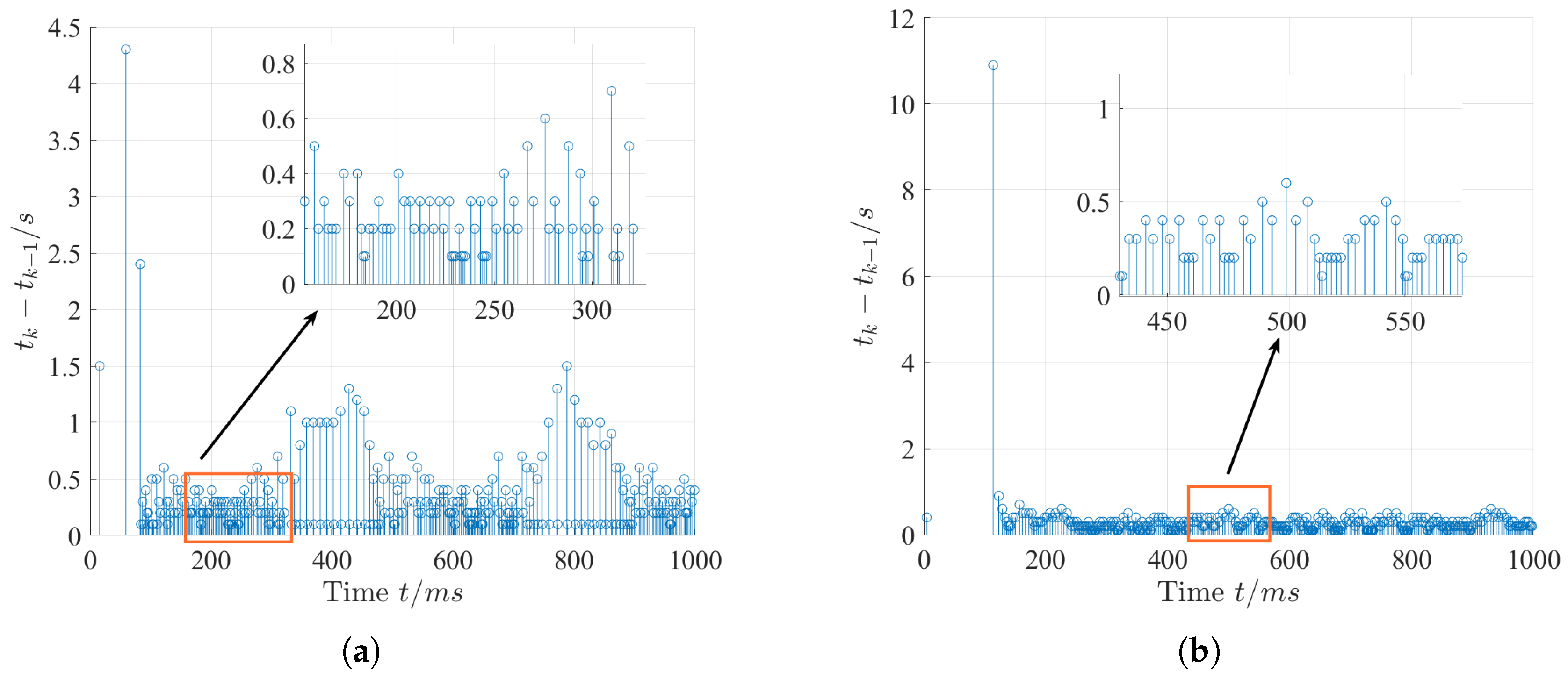
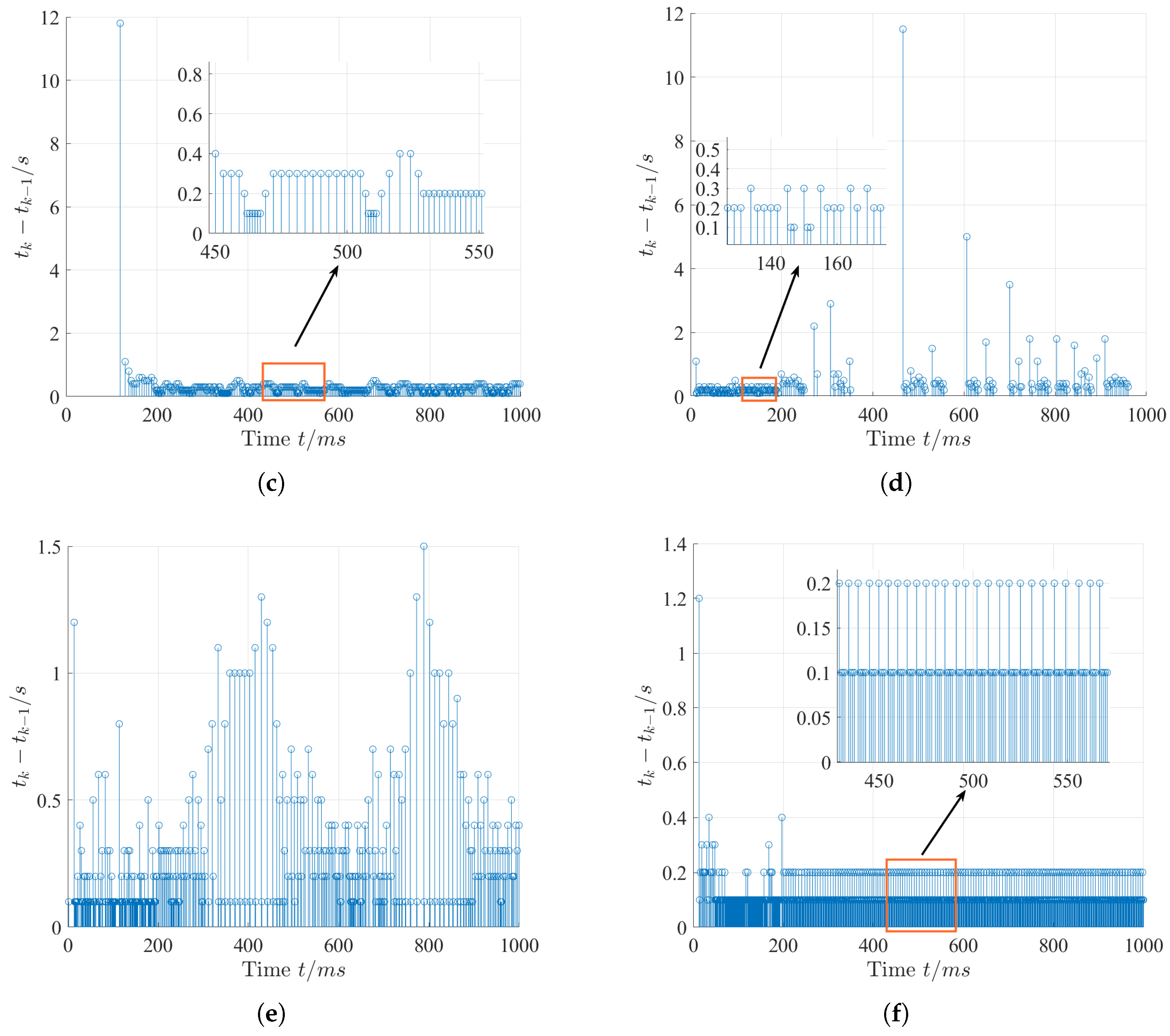
- Simulation: The classical scenarios are selected to demonstrate the effectiveness of EDLISMC, which includes a three-dimensional planar cosine trajectory and a three-dimensional spatial spiral trajectory. The relevant simulation proves that EDLISMC can achieve trajectory tracking control under the influence of reaction torque, the maximum triggering interval of the event triggering mechanism is 24 s.
2. Problem Description
- Condition 1: The estimation error of the system model and the time-varying external disturbances should be constrained. It can be defined as , where is an upper limit for external disturbances.
- Condition 2: The system model has an upper limit on reaction torque. It can be defined as , where is an upper limit for reaction torque.
- Condition 3: The system model has an upper limit on thrust. It can be defined as , where is an upper limit for thrust.
- Condition 4: The pitch angle of the UUV satisfies .
- Condition 5: The desired trajectories , , and of the UUV are limited.
3. The Proposed Method
3.1. Overall Structure
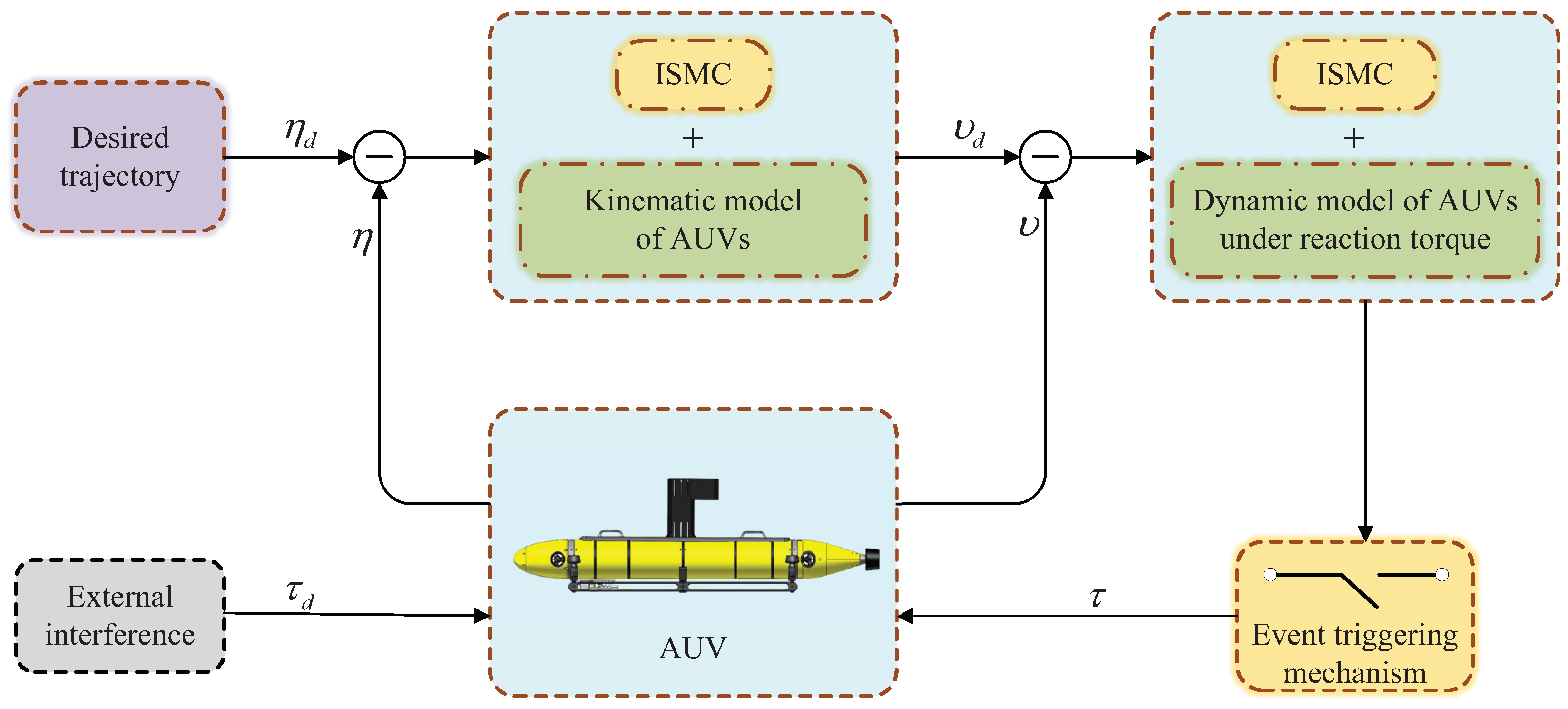
- 1.
- DLISMC includes the location loop controller and the speed loop controller. According to ISMC and the kinematic model of the UUV, the location loop controller realizes the tracking of location and attitude through the expected location and real-time location of the UUV. Then, the location loop controller outputs the reference speed as the input of the speed loop controller. Considering the time-varying ocean disturbances, the speed loop controller analyzes the dynamic model of the UUV under the influence of reaction torque.
- 2.
- The proposed event triggering mechanism determines whether to update the thrust output based on the output thrust of the speed loop. The ideal thrust of UUV is generated by EDLISMC. After the thruster is started, the UUV obtains real-time speed feedback to achieve precise tracking of the reference speed.
3.2. Dual-Loop Integral Sliding Mode Control Law
3.3. Event Triggering Mechanism
3.4. Zeno Behavior Analysis
4. Stability Analysis of Proposed Method
5. Simulation and Analysis
5.1. Simulation Setup
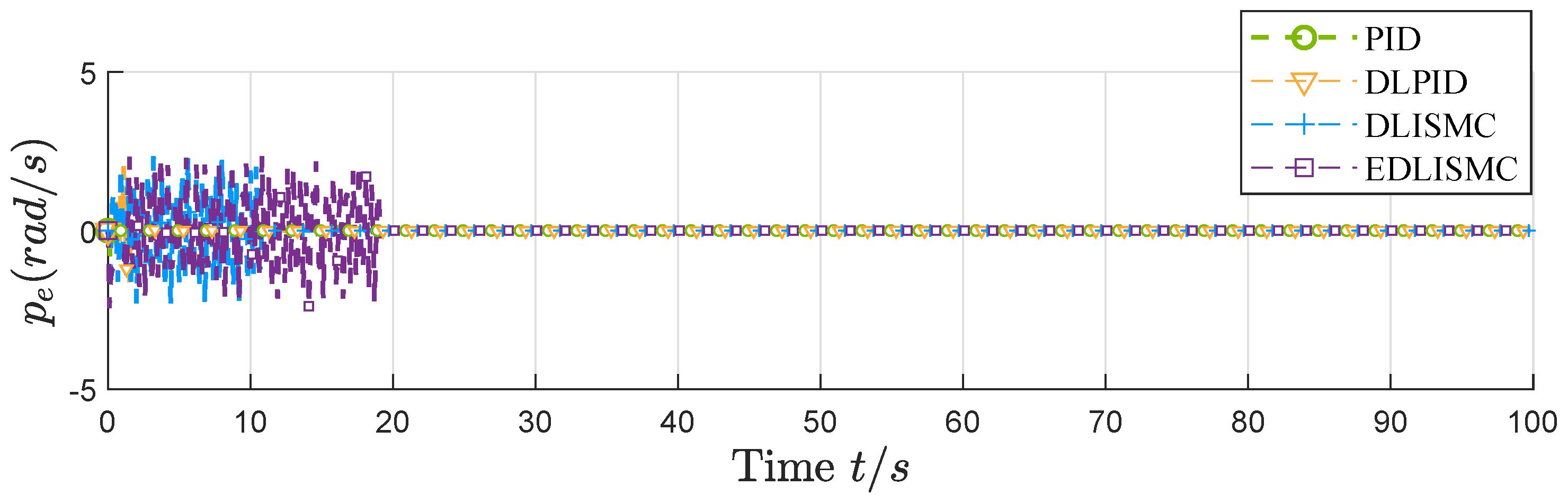
- To demonstrate the performance advantages of EDLISMC, this simulation experiment compares it with proportional integral derivative (PID) [28], dual-layer proportional integral derivative (DLPID) [29], and DLISMC. The location error and angle error of the UUV are the inputs of PID, and then the thrust magnitude of the UUV is obtained through proportional operation, integral operation, and differential operation of PID. DLPID is composed of a location loop controller and a speed loop controller, where the controllers are controlled by PID.
- Table 1 presents the parameter of the UUV mathematical model under reaction torque. The maximum thrust of UUV is set to ±200 N, and the time-triggered interval is 0.1 s. In addition, the simulation experiment of this paper introduces time-varying external disturbances with different amplitudes and periods, whose values can be expressed as
- To verify the feasibility of EDLISMC, this simulation experiment sets two trajectory tracking scenarios, which include three-dimensional planar cosine trajectory and three-dimensional spatial spiral trajectory. m, m, m, rad, rad, rad, m/s, and rad/s are set as the initial state of the UUV. In terms of parameter selection, this simulation experiment adopts the method of controlling variables to discuss the influence of parameters. After multiple parameter adjustments, this simulation experiment selects the appropriate control parameters. We obtain the main parameters of EDLISMC through extensive testing and the parameter selection of reference [30,31], which are summarized in Table 2.
5.2. Simulation Results
5.2.1. Results of Scenario 1
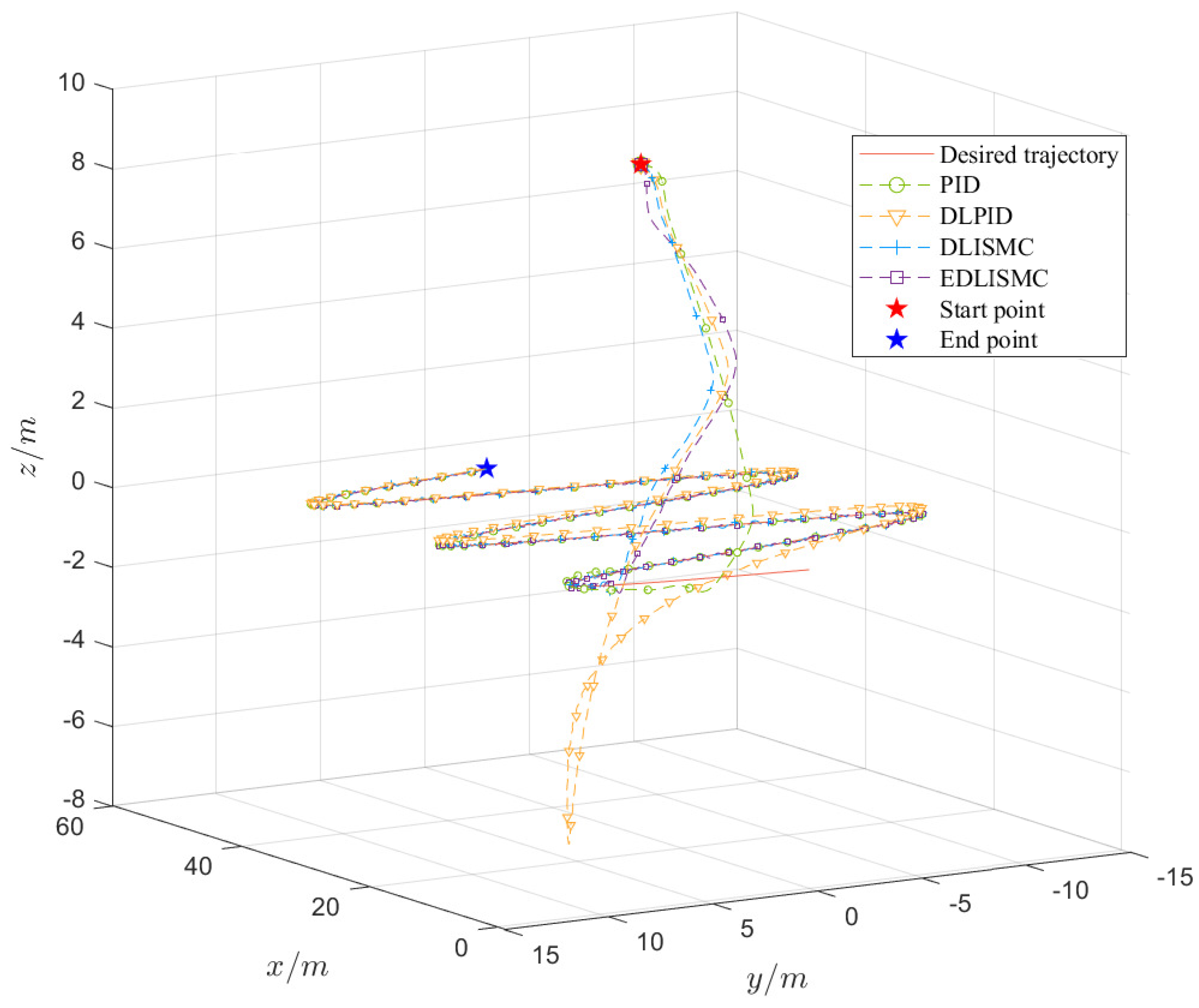
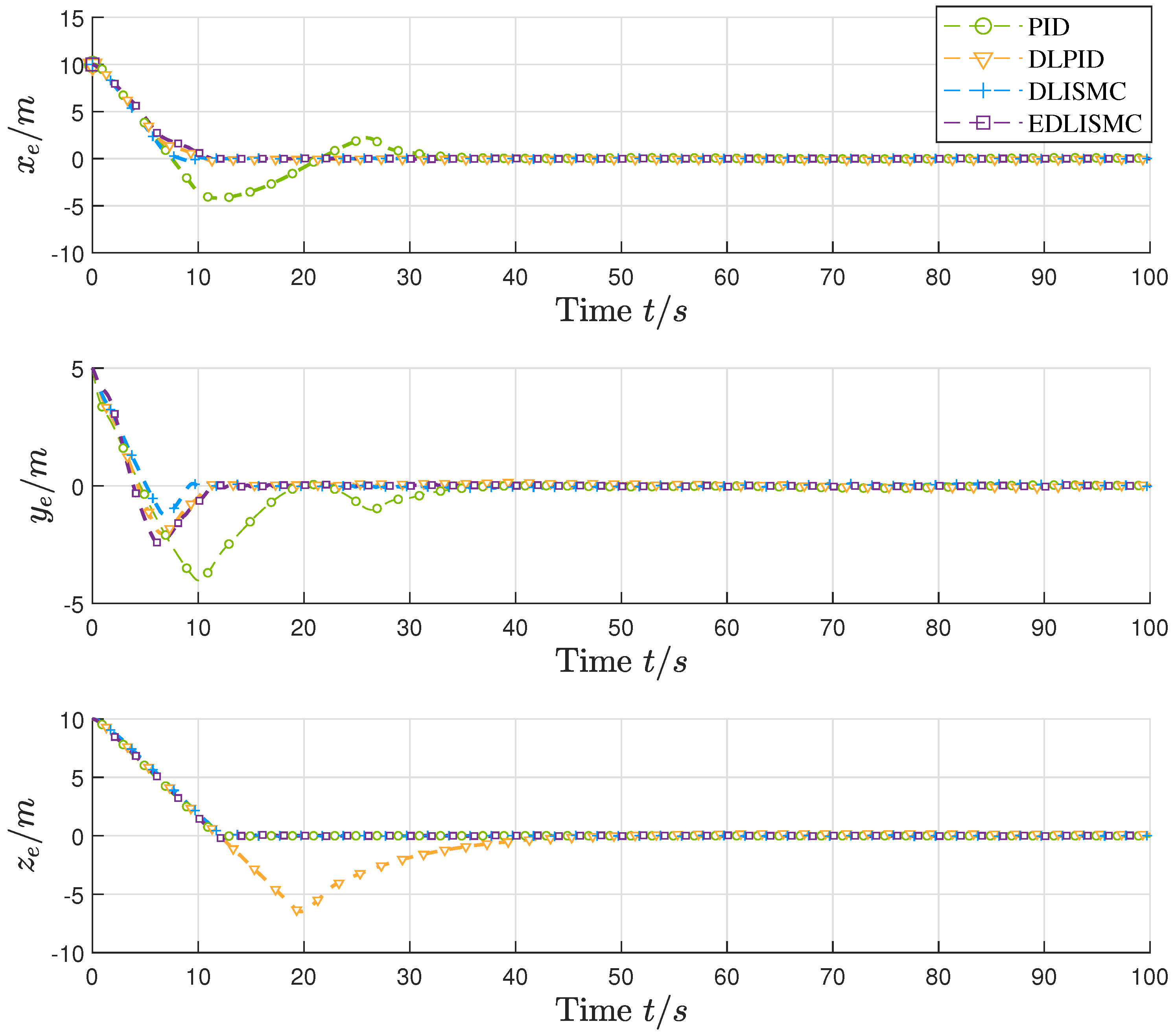
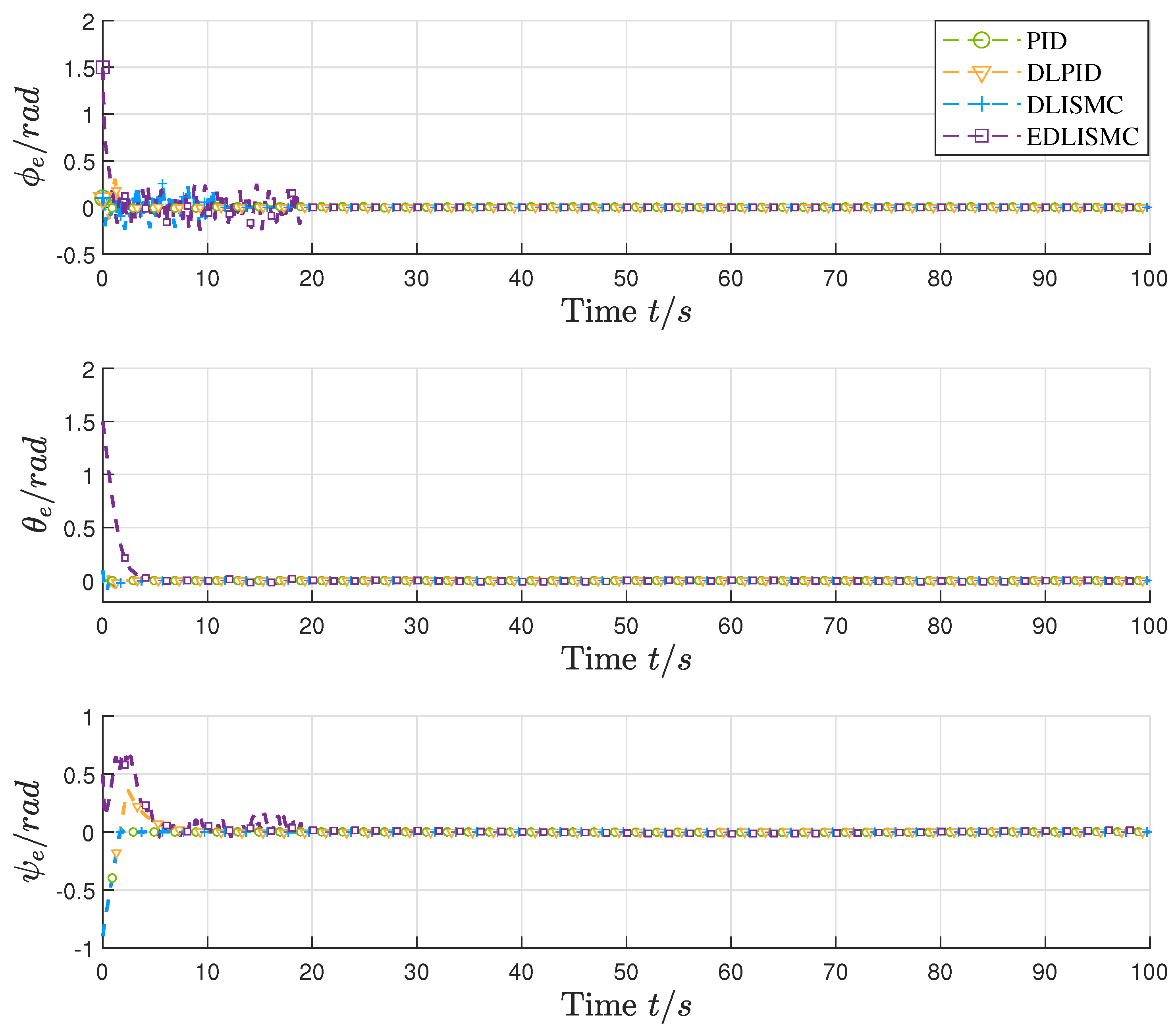
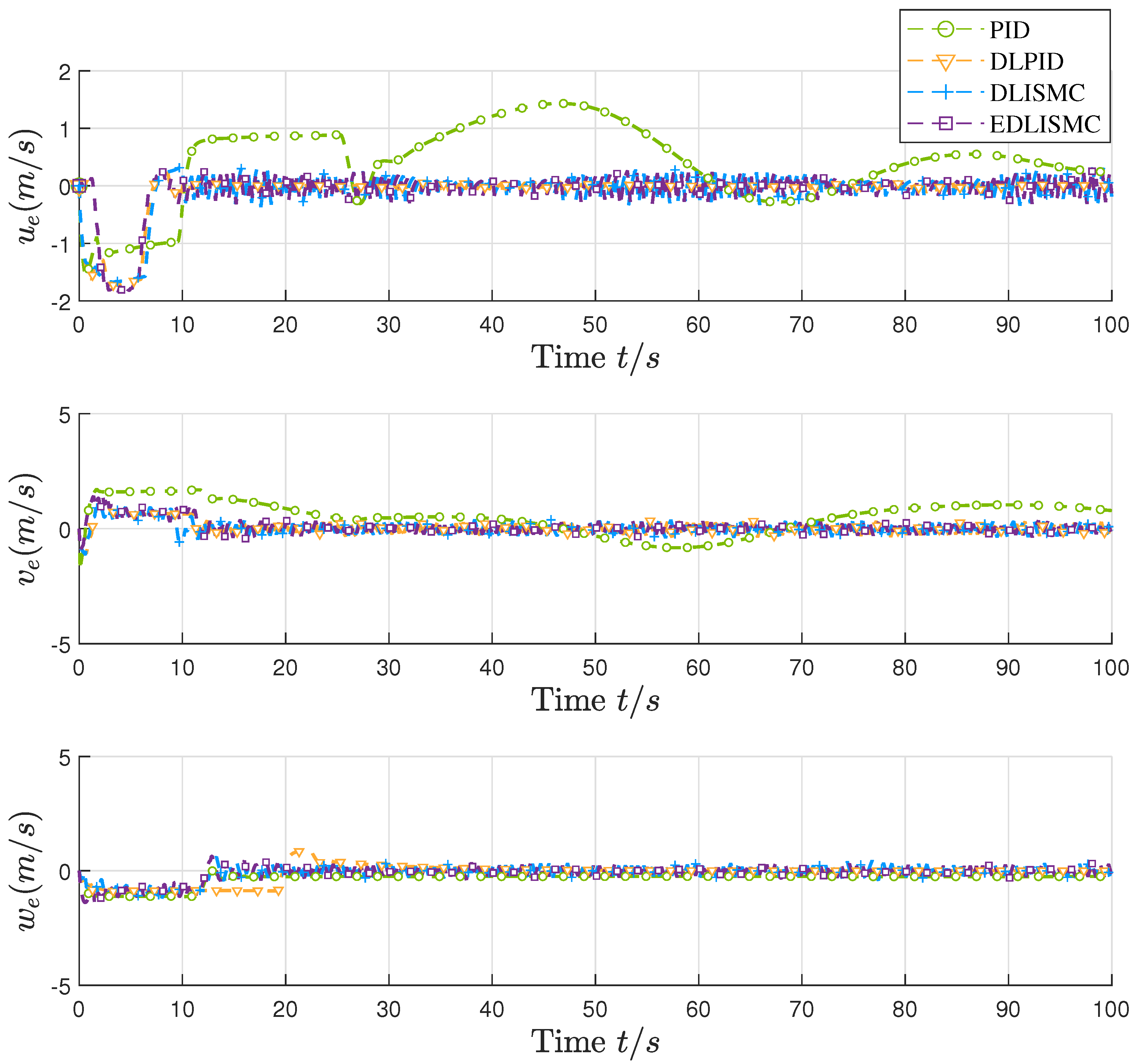
5.2.2. Results of Scenario 2
6. Conclusions
Author Contributions
Funding
Data Availability Statement
Conflicts of Interest
References
- Cai, W.; Chen, H.; Zhang, M. A cooperative hunting algorithm based on performance level classification for multi-autonomous underwater vehicle performance heterogeneity. J. Braz. Soc. Mech. Sci. Eng. 2025, 47, 1–16. [Google Scholar] [CrossRef]
- Wang, H.; Han, G.; Tang, D.; Xiong, W. Multi-AUV Collaboration-Assisted Location Privacy Protection Scheme in Unknown Marine Environments. IEEE Internet Things J. 2024, 11, 27398–27408. [Google Scholar] [CrossRef]
- Fayaz, S.; Parah, S.; Qureshi, J.; Lloret, J.; Del, J.; Muhammad, K. Intelligent underwater object detection and image restoration for autonomous underwater vehicles. IEEE Trans. Veh. Technol. 2023, 73, 1726–1735. [Google Scholar] [CrossRef]
- Zhu, X.; Khan, A.A.S.; Li, X. Global lumped mass formulation for underwater cable dynamics. Nonlinear Dyn. 2025, 113, 989–1006. [Google Scholar] [CrossRef]
- Er, M.J.; Gong, H.; Liu, Y.; Liu, T. Intelligent trajectory tracking and formation control of underactuated autonomous underwater vehicles: A critical review. IEEE Trans. Syst. Man Cybern. Syst. 2023, 54, 543–555. [Google Scholar] [CrossRef]
- Ma, D.; Chen, X.; Ma, W.; Zheng, H.; Qu, F. Neural Network Model-Based Reinforcement Learning Control for AUV 3-D Path Following. IEEE Trans. Intell. Veh. 2024, 9, 893–904. [Google Scholar] [CrossRef]
- Cui, J.; Hou, M.; Peng, Z.; Wang, Y.; Cui, J.H. Hamiltonian based AUV navigation using adaptive finite-time trajectory tracking control. Ocean Eng. 2025, 320, 1–17. [Google Scholar] [CrossRef]
- Li, X.; Liu, Y. A new fuzzy SMC control approach to path tracking of autonomous underwater vehicles with mismatched disturbances. In Proceedings of the OCEANS 2022, Chennai, India, 21–24 February 2022; pp. 1–5. [Google Scholar]
- Zhang, W.; Wang, Q.; Du, X.; Zheng, Y. Real-time NMPC for three-dimensional trajectory tracking control of AUV with disturbances. Ocean Eng. 2025, 319, 1–13. [Google Scholar] [CrossRef]
- Wan, L.; Zhang, Y.; Sun, Y.; Li, Y.; He, B. ADRC Path-Following Control of Underactuated AUVs. J. Shanghai Jiao Tong Univ. 2014, 48, 1727–1731. [Google Scholar]
- Ye, H.; Wang, L.; Zhi, P.; Zhu, D. Adaptive three-dimensional path tracking control for AUV based on disturbance observer. J. Jiangsu Univ. Sci. Technol. (Nat. Sci. Ed.) 2019, 33, 52–59. [Google Scholar]
- Wang, Y.; Hou, Y.; Lai, Z.; Cao, L.; Hong, W.; Wu, D. An expert-demonstrated soft actor–critic based adaptive trajectory tracking control of Autonomous Underwater Vehicle with Long Short-Term Memory. Ocean Eng. 2025, 321, 1–11. [Google Scholar] [CrossRef]
- Li, G.; Li, J.; Zhong, R.; Xie, H.; Dan, Y.; Hou, C. An AUV Control Method Based on Modified Super-Twisting Sliding Mode and Disturbance Observer. Digit. Ocean. Underw. Warf. 2023, 6, 300–307. [Google Scholar]
- Li, J.; Xia, Y.; Xu, G.; Guo, Z.; Han, H.; Wu, Z.; Xu, K. Enhanced three-dimensional trajectory tracking control for AUVs in variable operating conditions using FMPC-FTTSMC. Ocean Eng. 2024, 310, 1–19. [Google Scholar] [CrossRef]
- Xu, X.; He, B.; Dai, N.; Wang, T.; Shen, Y. Tracking control study of AUV large curvature path based on artificial physics method. Ocean Eng. 2024, 303, 1–15. [Google Scholar] [CrossRef]
- Li, B.; Gao, X.; Huang, H.; Yang, H. Improved adaptive twisting sliding mode control for trajectory tracking of an AUV subject to uncertainties. Ocean Eng. 2024, 297, 1–12. [Google Scholar] [CrossRef]
- Chen, P.; Yu, L.; Guo, K.; Qiao, L. Fast and Accurate Trajectory Tracking Control for Underactuated AUVs With Mismatched Disturbances: Theory and Experiment. IEEE Trans. Ind. Electron. 2025, 99, 1–10. [Google Scholar] [CrossRef]
- Fenco Bravo, L.P.; Pérez Zuñiga, C.G. Nonlinear trajectory tracking with a 6DOF AUV using an MRAFC controller. IEEE Lat. Am. Trans. 2025, 23, 160–171. [Google Scholar] [CrossRef]
- Ebrahimpour, M.; Lungu, M. Finite-Time Path-Following Control of Underactuated AUVs with Actuator Limits Using Disturbance Observer-Based Backstepping Control. Drones 2025, 9, 70. [Google Scholar] [CrossRef]
- Xu, F.; Zhang, L.; Zhong, J. Three-dimensional path tracking of over-actuated AUVs based on mpc and variable universe s-plane algorithms. J. Mar. Sci. Eng. 2024, 12, 418. [Google Scholar] [CrossRef]
- Yu, G.; He, F.; Liu, H. Fuzzy neural network adaptive AUV control based on FTHGO. Sh. Offshore Struct. 2025, 20, 13–25. [Google Scholar] [CrossRef]
- Miao, J.; Wang, S.; Zhao, Z.; Li, Y.; Tomovic, M.M. Spatial curvilinear path following control of underactuated AUV with multiple uncertainties. ISA Trans. 2017, 67, 107–130. [Google Scholar] [CrossRef] [PubMed]
- Al Makdah, A.A.R.; Daher, N.; Asmar, D.; Shammas, E. Three-dimensional trajectory tracking of a hybrid autonomous underwater vehicle in the presence of underwater current. Ocean Eng. 2019, 185, 115–132. [Google Scholar] [CrossRef]
- Pan, Y.; Yang, C.; Pan, L.; Yu, H. Integral sliding mode control: Performance, modification, and improvement. IEEE Trans. Ind. Inform. 2017, 14, 3087–3096. [Google Scholar] [CrossRef]
- Abidi, K.; Xu, J.X.; Xinghuo, Y. On the discrete-time integral sliding-mode control. IEEE Trans. Autom. Control 2007, 52, 709–715. [Google Scholar] [CrossRef]
- Song, L.; Tong, S. Finite-time resilient integral sliding-mode control for fuzzy impulsive stochastic system under denial-of-service attacks. IEEE Trans. Fuzzy Syst. 2024, 32, 2930–2939. [Google Scholar] [CrossRef]
- Binh, T.N.; Huu Sau, N.; Thi Thanh Huyen, N.; Thuan, M.V. Guaranteed cost control of delayed conformable fractional-order systems with nonlinear perturbations using an event-triggered mechanism approach. Int. J. Syst. Sci. 2025, 74, 1–18. [Google Scholar] [CrossRef]
- Liu, G.P. Tracking control of multi-agent systems using a networked predictive PID tracking scheme. IEEE/CAA J. Autom. Sin. 2023, 10, 216–225. [Google Scholar] [CrossRef]
- Ji, Y.; Zhang, J.; Zhang, J.; He, C.; Hou, X.; Han, J. Constraint performance slip ratio control for vehicles with distributed electrohydraulic brake-by-wire system. Proc. Inst. Mech. Eng. Part D J. Automob. Eng. 2024, 238, 1861–1879. [Google Scholar] [CrossRef]
- Guerrero, J.; Torres, J.; Creuze, V.; Chemori, A. Adaptive disturbance observer for trajectory tracking control of underwater vehicles. Ocean Eng. 2020, 200, 107080. [Google Scholar] [CrossRef]
- Herman, P. Numerical Test of Several Controllers for Underactuated Underwater Vehicles. Appl. Sci. 2020, 10, 8292. [Google Scholar] [CrossRef]


| Parameter | Value | Unit | Parameter | Value | Unit |
|---|---|---|---|---|---|
| 125 | k | 0.027 | / | ||
| 0.05 | m | 0.063 | / | ||
| g | 9.81 | m/s2 | 230 | N·s2/m | |
| 4.63 | kg·m2 | 280 | N·s2/m | ||
| 4.63 | kg·m2 | 100 | N(s/m)2v | ||
| 4.63 | kg·m2 | 148 | N(s/m)2 | ||
| 4.63 | kg·m2 | 4.63 | kg·m2 | ||
| 4.63 | kg·m2 |
| Parameter | Value | Parameter | Value | Parameter | Value |
|---|---|---|---|---|---|
| 0.00001 | 100,000 | 10 | |||
| 0.00001 | 100,000 | 0.01 | |||
| 0.0001 | 900,000 | 1.2 | |||
| 0.01 | 5 | 0.001 | |||
| 0.01 | 0.5 | 1 | |||
| 10 | 5 | 1 | |||
| 0.001 | 100 | 0.5 | |||
| 0.001 | 0.1 | 0.01 | |||
| 0.001 | 0.1 |
| Triggering Item | Triggering Count | Event Triggering Count/Time Triggering Count |
|---|---|---|
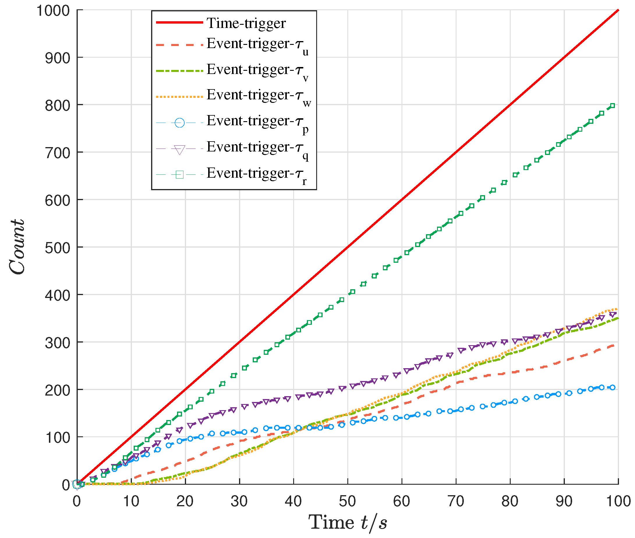
| Time triggering mechanism | 1000 | / |
| 296 | 29.6% | |
| 351 | 35.1% | |
| 370 | 37.0% | |
| 204 | 20.4% | |
| 362 | 36.2% | |
| 807 | 80.7% |
| Triggering Item | Triggering Count | Event Triggering Count/Time Triggering Count |
|---|---|---|
| Time triggering mechanism | 1000 | / |
| 276 | 27.6% | |
| 313 | 31.3% | |
| 354 | 35.4% | |
| 70 | 7% | |
| 282 | 28.2% | |
| 785 | 78.5% |
Disclaimer/Publisher’s Note: The statements, opinions and data contained in all publications are solely those of the individual author(s) and contributor(s) and not of MDPI and/or the editor(s). MDPI and/or the editor(s) disclaim responsibility for any injury to people or property resulting from any ideas, methods, instructions or products referred to in the content. |
© 2025 by the authors. Licensee MDPI, Basel, Switzerland. This article is an open access article distributed under the terms and conditions of the Creative Commons Attribution (CC BY) license (https://creativecommons.org/licenses/by/4.0/).
Share and Cite
Ju, Y.; Cai, W.; Zhang, M.; Chen, H. A Trajectory Tracking Control Method for 6 DoF UUV Based on Event Triggering Mechanism. J. Mar. Sci. Eng. 2025, 13, 879. https://doi.org/10.3390/jmse13050879
Ju Y, Cai W, Zhang M, Chen H. A Trajectory Tracking Control Method for 6 DoF UUV Based on Event Triggering Mechanism. Journal of Marine Science and Engineering. 2025; 13(5):879. https://doi.org/10.3390/jmse13050879
Chicago/Turabian StyleJu, Yakang, Wenyu Cai, Meiyan Zhang, and Hao Chen. 2025. "A Trajectory Tracking Control Method for 6 DoF UUV Based on Event Triggering Mechanism" Journal of Marine Science and Engineering 13, no. 5: 879. https://doi.org/10.3390/jmse13050879
APA StyleJu, Y., Cai, W., Zhang, M., & Chen, H. (2025). A Trajectory Tracking Control Method for 6 DoF UUV Based on Event Triggering Mechanism. Journal of Marine Science and Engineering, 13(5), 879. https://doi.org/10.3390/jmse13050879