Multi-Objective Path Optimization Method for Maritime UAVs Equipped with Inertial Navigation Systems

Abstract

Maritime unmanned aerial vehicles (UAVs) equipped with inertial navigation systems (INS) are prone to error accumulation, which can lead to excessive positioning errors and hinder their ability to perform long distance missions. To address this issue, this study first constructs a directed graph network for a flight area based on start and end points as well as error correction points. A multi-objective route planning model is then developed for a UAV, aiming to minimize both the flight distance and the number of positioning corrections. Considering the UAV’s turning radius, a trajectory length calculation model based on 3D Dubins curves is designed. Subsequently, a forward labeling-based multi-objective path planning algorithm is proposed to develop an optimization model. Experimental results demonstrate that the proposed method can effectively constrain the UAV’s horizontal and vertical positioning errors within 2.5 m, while optimally balancing flight distance and positioning accuracy to ensure the successful execution of long-range maritime UAV missions. The comparative results demonstrate that, while satisfying the positioning error requirements, our proposed method achieves a reduction of over 1.5% in total flight distance for maritime UAVs compared to the NSGA-II algorithm.

1. Introduction

Maritime unmanned aerial vehicles (UAVs) exhibit high flexibility, maneuverability, and relatively low cost. With advancements in UAV and sensor technologies, the application scenarios for maritime UAVs have been further expanded [1]. Currently, maritime UAVs are widely utilized in various fields, including maritime search and rescue [2], ocean monitoring [3], maritime network communication [4], maritime target localization [5], marine debris detection [6], and marine species monitoring [7]. Compared to traditional maritime operations, the use of maritime UAVs enables efficient information collection and task execution in complex marine environments, providing robust technical support for maritime safety and environmental protection.

Numerous scholars have conducted research on UAV path optimization. Classical algorithms commonly used for UAV path planning include Dijkstra’s algorithm [8], artificial potential fields [9], rapidly exploring random trees (RRTs) [10], visibility graph algorithms [11], and probabilistic road map algorithms [12]. These classical methods typically rely on complete prior knowledge of the environment and exhibit high computational complexity, presenting significant limitations in practical application [1].

Dynamic programming algorithms are also frequently employed in path planning. Mokrane et al. [13] proposed a three-dimensional path planning method based on dynamic programming, utilizing a digital elevation model (DEM) generated through photogrammetry to plan optimal trajectories. Bauso et al. [14] synthesized a local predictive controller based on a distributed and scalable suboptimal neural dynamic programming (NDP) algorithm. This algorithm discretizes space using Voronoi diagrams and estimates the formation center position through a consensus protocol, thereby achieving path planning. Radmanesh et al. [15] transformed the path planning problem into a fast dynamic mixed-integer linear programming (MILP) problem, optimizing UAV flight paths by defining cost functions and constraints. This approach enables UAV formations to maintain their configuration while effectively avoiding moving obstacles and minimizing flight time and energy consumption. However, multi-objective optimization problems in complex systems often involve nonlinearity, non-differentiability, multimodality, discontinuity, non-separability, and inequality constraints. When problem complexity is high, traditional mathematical programming algorithms may struggle to provide solutions [16,17].

Commonly used heuristic algorithms include the A* algorithm and its variants, as well as greedy algorithms. Bayili and Polat [18] proposed the novel Limited-Damage A* (LDA*) algorithm, which considers both path length and path damage as feasibility criteria, making it suitable for safety-aware path search problems. Chen et al. [19] improved the traditional A* algorithm based on a mixed-integer linear programming (MILP) model by introducing the cosine value of vector angles to optimize the evaluation function, thereby reducing the number of search nodes and improving search efficiency. Meng [20] proposed an enhanced A* algorithm for UAV path planning. By introducing a new heuristic function and optimizing node selection strategies, this algorithm demonstrates excellent performance in high-obstacle-density environments. Aslan [21] introduced a greedy algorithm named Back-and-Forth (BaF) for solving UAV geometric path planning problems. Compared with 14 metaheuristic-based path planning algorithms, the BaF algorithm was shown to generate superior or at least comparable paths.

Metaheuristic algorithms can be categorized into evolutionary algorithms (EAs), physics-based algorithms, and swarm intelligence (SI) algorithms [22]. Duan et al. [23] proposed a hybrid metaheuristic algorithm combining ant colony optimization and differential evolution for UAV three-dimensional path planning, enabling rapid generation of feasible 3D paths in complex environments. Zhao et al. [24] (2024) introduced a clustering-based hyper-heuristic algorithm that leverages graph neural networks to learn heuristic indicators and integrates reinforcement learning with ant colony optimization to optimize paths, thereby avoiding the limitations of expert experience and suboptimal manual parameter tuning. Wu et al. [25] (2024) proposed the improved Aquila Optimization algorithm based on particle swarm optimization (PSO), incorporating PSO’s self-learning and social learning mechanisms into the local exploitation phase of the Aquila Optimization algorithm to prevent premature convergence to global optima, making it suitable for various complex optimization scenarios. Li et al. [26] developed an enhanced path planning algorithm combining K-means clustering and genetic algorithms (GAs), effectively narrowing the search space and making it applicable to large-scale data processing and real-world scenarios.

With the advancement of data science, technologies such as deep learning and reinforcement learning have rapidly emerged and been widely applied across various fields, including UAV path planning. Boulares et al. [27] designed an algorithm combining target trajectory prediction and regression analysis, optimizing the accuracy and stability of predicted trajectories by comparing regularization techniques such as lasso, ridge, and elastic net. Boulares et al. [28] proposed a UAV path planning algorithm based on deep Q-learning, transforming the UAV path planning problem into a Markov decision process (MDP) and training it using deep Q-learning. He et al. [29] introduced a deep neural network (DNN) reactive controller combining convolutional neural networks (CNNs) and fully connected networks (FCNs), trained using the Twin Delayed DDPG (TD3) algorithm and analyzed for interpretability using SHAP.

However, the above studies focus solely on UAVs equipped with GPS positioning systems. In practice, due to the scarcity of positioning base stations in maritime environments, patrol UAVs typically rely on INS systems, whose errors accumulate over time. Consequently, the methods proposed in prior studies fail to account for the error accumulation effect of INS, making it difficult to ensure that planned trajectories will enable maritime UAVs to successfully complete patrol missions. To bridge this gap, this study aims to develop a multi-objective path optimization method for INS-equipped maritime UAVs, balancing path lengths and positioning errors to ensure reliable mission execution.

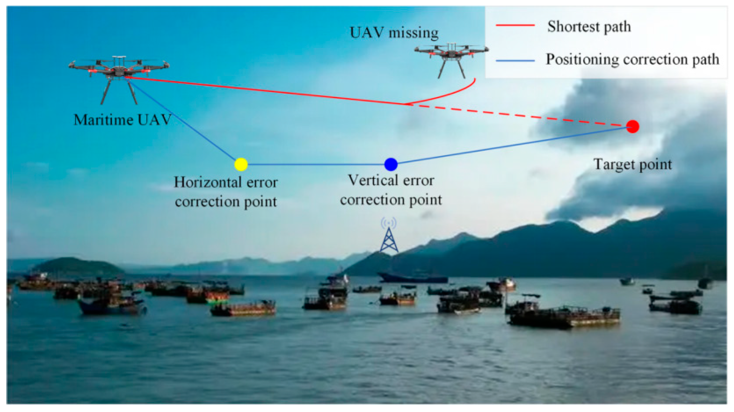
2. Problem Description

Due to the limitations of the maritime environment, UAVs often rely on INS rather than GPS to ensure positioning accuracy. However, INS calculates position, velocity, and attitude by measuring acceleration and angular velocity. Since it operates autonomously without external references, errors accumulate over time, a phenomenon known as error drift. During long-distance flights, both vertical and horizontal errors increase with flight distance. To address this, maritime UAVs typically use known reference points as correction points to mitigate the error drift of INS. As illustrated in Figure 1, the red and blue trajectories represent a UAV’s shortest path and correction path, respectively. The yellow points denote horizontal error correction points, while the blue points indicate vertical error correction points. If the vertical or horizontal errors exceed critical thresholds along the shortest path, the UAV may fail its mission or even be lost.

Considering a more general scenario, as illustrated in Figure 2, there may be numerous correction points within the navigation area. The error correction points for UAVs, serving as high-precision markers with coordinates measured by total stations or similar instruments, represent one of the conventional approaches for rectifying positioning errors in INS systems. By timely correction of both vertical and horizontal errors, the UAV can follow the planned route, reaching its destination after passing through several correction points. However, increasing the number of corrections often reduces operational efficiency. Therefore, this study aims to optimize the UAV’s path by minimizing both the number of corrections and the total path length, thereby identifying the most efficient flight plan.

3. Mathematical Model

3.1. Model Assumptions

For the purpose of facilitating the modeling process, the following assumptions are proposed:

(1)

At the starting point, the vertical and horizontal errors of the aircraft are both zero.

(2)

When the UAV performs vertical error correction at a vertical error correction point, its vertical error is reset to 0, while the horizontal error remains unchanged.

(3)

When the UAV performs horizontal error correction at a horizontal error correction point, its horizontal error is reset to 0, while the vertical error remains unchanged.

(4)

During flight, the UAV operates without unexpected disruptions, except as specified in the problem statement.

(5)

The UAV can continue to follow the planned trajectory provided that both the vertical and horizontal errors remain below their critical thresholds.

3.2. Model Variables and Parameters

The main variables and parameters are listed in

Table 1. Definition of Formula Symbols.

Parameters	Meanings
G = (V,E)	Directed graph.
V	Point set, |V| = n, including the starting point A, the target point B, and the correction points.
E	Edge set, |E| = m, the set of edges between points.
Vver	The set of vertical error correction points.
Vhor	The set of horizontal error correction points.
i, j	The node sequence, in a given path, j is the next node corresponding to i.
k	Intermediate point between i, j on Dubins curve.
(i, j)	An edge from i to j.
R	R={2, …, L}, representing the set of feasible path edge counts.
r	Sequence of edges in a path.
Pi	The set of reachable points corresponding to point i.
dij	The length of the edge from node i to j, i.e., the distance between i and j, m.
ηijver ηijhor	The vertical error and horizontal error from i to j.
δ	For every 1 m of flight, the vertical and horizontal error increments of the UAVs.
θ	Upon reaching the end point, the maximum values of vertical and horizontal errors.
α1, α2	The upper bounds for both vertical and horizontal errors, if vertical errors can be corrected.
β1, β2	The upper bounds for both vertical and horizontal errors, if horizontal errors can be corrected.
M	Minimum turning radius of the UAV, m.
xrij	The binary variable xrij is defined such that xrij = 1 if the edge (i,j) is the r-th segment of a feasible path; otherwise, xrij = 0.

.

3.3. Maritime UAV Path Planning Model

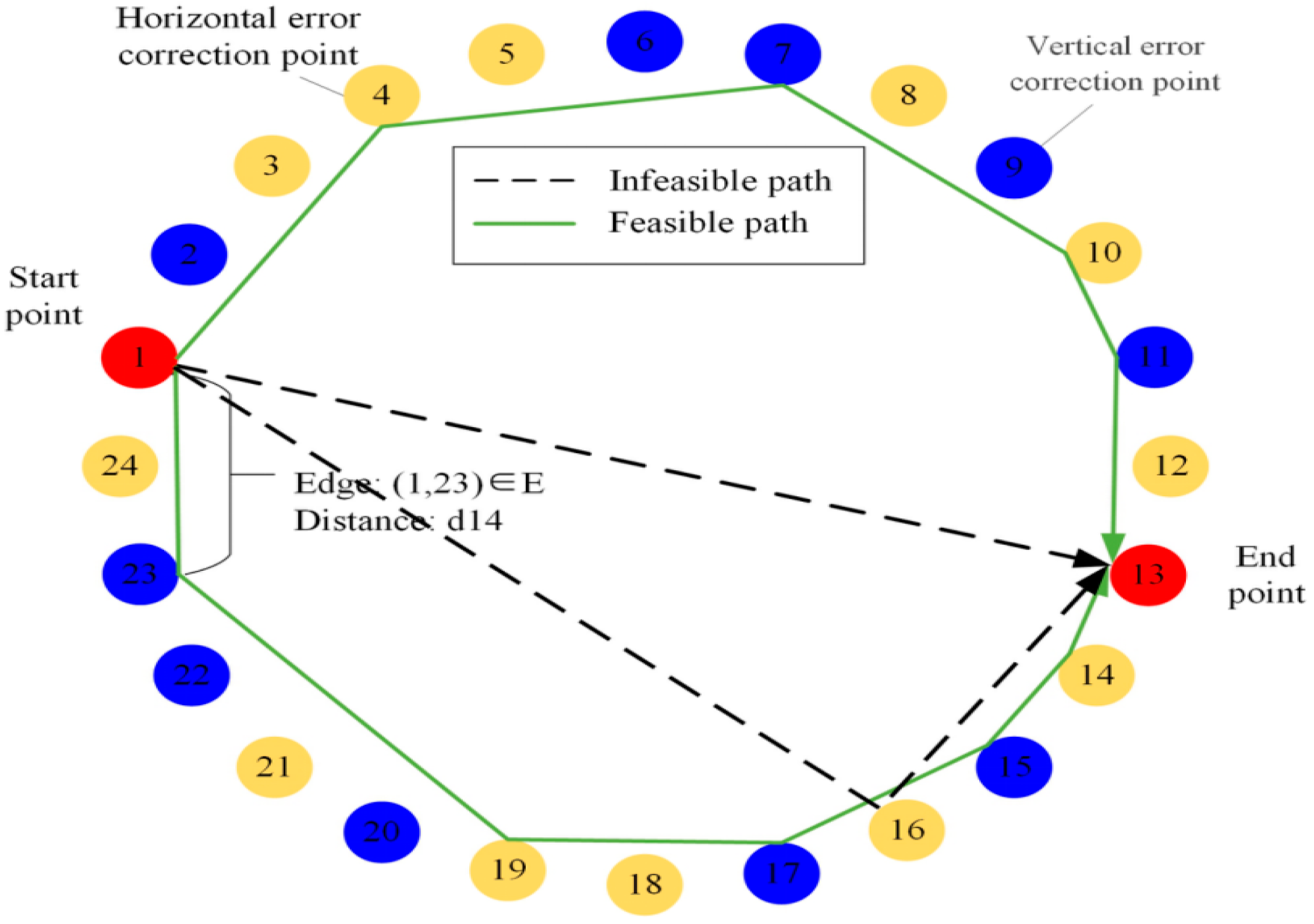
3.3.1. Directed Graph Network

The pairwise connections between points in the space form a directed graph. The path planning problem for maritime UAVs is thus formulated as finding a feasible path within this directed graph that minimizes both the trajectory length and the number of required corrections. Set G = (V,E), and then a network representation of drone path planning, encompassing 24 nodes, can be illustrated in Figure 3. The black dashed line represents the shortest flight route. If the drone follows this route, it may lose its way due to excessive positioning errors. The orange line segment represents the positioning correction route. The drone can successfully reach the target point after passing through multiple correction points.

Based on the directed graph constructed, a multi-objective optimization model can be established as follows:

$$\mathrm{m}\mathrm{i}\mathrm{n}F=\left(F_1,F_2\right)$$

(1)

The trajectory length is described as follows:

$$F_1\left(x_{ij}^r\right)={\sum }_{r\in R}{\sum }_{\left(i,j\right)\in E}{x}_{ij}^r\cdot d_{ij}$$

(2)

The number of trajectory corrections is described as follows:

$$F_2\left(x_{ij}^r\right)={\sum }_{r\in R}{\sum }_{\left(i,j\right)\in E}{x}_{ij}^r$$

(3)

Therefore, it is essential to evaluate the distances between waypoints and assess their reachability, particularly to determine whether the cumulative error threshold may be exceeded.

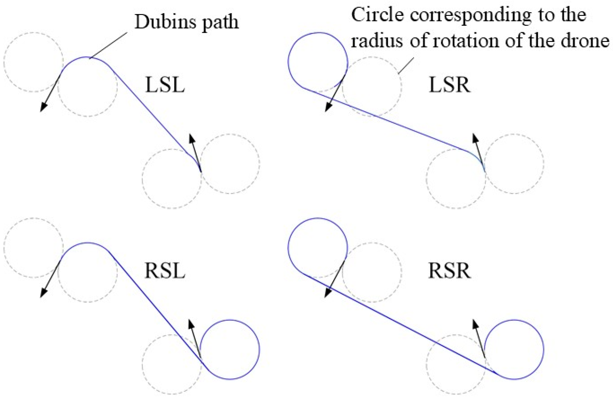
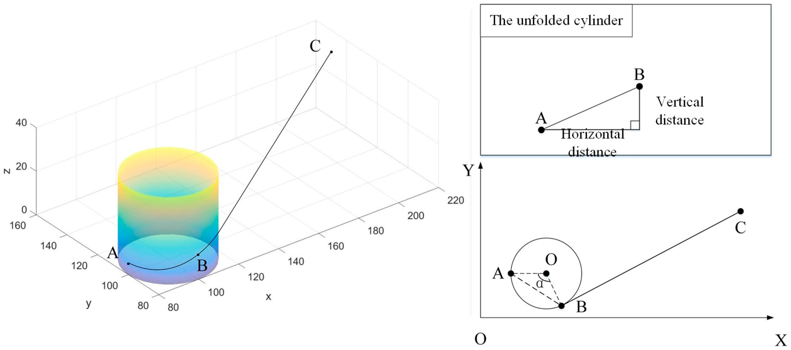
3.3.2. Path Distance Calculation Based on Dubins Curve

Due to the minimum turning radius constraint, UAVs cannot perform instantaneous turns and instead adjust their direction by following circular arcs. In this process, both the pre-turn and post-turn directions are tangent to the arc. For a given flight path consisting of multiple nodes, minimizing the trajectory length primarily involves addressing two key issues: (1) determining the optimal allocation strategy between straight segments and circular arcs in the trajectory, and (2) identifying the appropriate radius of the circular arcs.

In this study, Dubins curves are employed to determine the optimal combination of circular arcs and straight segments in the flight trajectory. Using geometric principles, it is proven that the trajectory length is minimized when the radius of the circular arcs equals the minimum turning radius of 200 m. Based on this finding, a recursive equation for calculating the trajectory length is derived, leading to the development of a 3D Dubins curve-based trajectory length computation method.

To better understand the significance of the turning radius constraint, a control model of the aircraft is first established. The aircraft’s attitude at a specific position is described using l(x, y, z, θ, $\phi$), where (x, y, z) represents the three-dimensional positional variables of the aircraft, θ denotes the horizontal turning angle, and Ψ represents the vertical climb or descent angle. Therefore, the trajectory of the aircraft along a feasible path can be regarded as a collection of a series of aircraft attitudes. The planning problem can thus be transformed into finding a set of aircraft control schemes that minimize the trajectory length while reducing the number of corrections as much as possible. The aircraft’s trajectory can be determined by the control set. If the state is a continuous function, it can be expressed as

$$L\left(x,y,z,q,\phi \right)={\int }_A^{B}l\left(x,y,z,q,\phi \right)$$

(4)

$$L\left(x,y,z,q,\phi \right)\Rightarrow Pat{h}_A\to Pat{h}_B$$

(5)

where L represents the set of l, and PathA→PathB denotes the path from the starting point A to the target point B.

It is evident that the aircraft may also undergo horizontal turns during the climb. Therefore, the resulting trajectory should be a curve with continuously varying curvature, forming a clothoid-like path. Numerous scholars have investigated this issue, with most employing Dubins curves to smooth the aircraft’s trajectory. Accordingly, this paper utilizes Dubins curves to construct a corresponding three-dimensional Dubins trajectory, which consists of a combination of straight lines and helical segments from the starting point to the endpoint. Dubins paths for UAVs are categorized into four distinct cases: LSL, LSR, RSL, and RSR, as illustrated in Figure 4. The selection of an appropriate path is determined by the relative positioning of the moving object’s initial and final configurations.

When a cylinder is unfolded, the helical path on its surface transforms into a straight line. A schematic diagram of this unfolding process is shown in Figure 5.

The length of the track from A to C is

$$d_{AC}=\sqrt{{l_{AB}}^2+{\left(x_C-x_B\right)}^2+{\left(y_C-y_B\right)}^2+{\left(z_C-z_A\right)}^2}$$

(6)

$$l_{AB}={\displaystyle \frac{\pi r}{90}}\cdot \mathrm{a}\mathrm{r}\mathrm{c}\mathrm{s}\mathrm{i}\mathrm{n}\left[{\displaystyle \frac{\sqrt{{\left(x_B-x_A\right)}^2+{\left(y_B-y_A\right)}^2}}{2M}}\right]$$

(7)

The partial derivation of dAC with respect to r yields

$${\displaystyle \frac{\partial d_{AC}}{\partial R}}=\left({\displaystyle \frac{\pi }{90}}-{\displaystyle \frac{\pi }{90r}}\right)\cdot \mathrm{a}\mathrm{r}\mathrm{c}\mathrm{s}\mathrm{i}\mathrm{n}\left[{\displaystyle \frac{\sqrt{{\left(x_B-x_A\right)}^2+{\left(y_B-y_A\right)}^2}}{2M}}\right]$$

(8)

Since R is greater than the minimum turning radius of UAVs, thus $\partial {\mathrm{d}}_{\mathrm{A}\mathrm{C}}/\partial \mathrm{r}>0$, that is, as the turning radius R increases, the trajectory length also increases. Therefore, R should be set to the minimum turning radius of the UAV to ensure optimal path efficiency. Furthermore, if the coordinates of points A, B, and C are known, the trajectory length from A to C can be calculated accordingly. Therefore, for a given UAV trajectory, its path length can be expressed as follows:

$$d_{ij}=\sqrt{\left({\displaystyle \frac{\pi r}{90}}\cdot \mathrm{a}\mathrm{r}\mathrm{c}\mathrm{s}\mathrm{i}\mathrm{n}\left[{\displaystyle \frac{\sqrt{{\left(x_k-x_i\right)}^2+{\left(y_k-y_i\right)}^2}}{2M}}\right]\right){l_{ij}}^2+{\left(x_j-x_k\right)}^2+{\left(y_j-y_k\right)}^2+{\left(z_j-z_i\right)}^2}$$

(9)

3.3.3. Uncertainty of Calibration Error

The flight environment of the UAV may change dynamically over time. Although the correction points are predetermined before the flight, the UAV may not achieve ideal error correction (i.e., reducing a specific error to zero) at certain correction points due to uncontrollable factors such as weather conditions, which can hinder the effectiveness of the correction process. Regarding error correction at designated points, there exists a probability that errors are either fully corrected to zero or partially corrected to min (error,5) units. To simultaneously maximize the probability of successfully reaching the destination, the problem involves three objectives: minimizing trajectory length, minimizing the number of correction points, and maximizing success probability. Consequently, the core challenge lies in establishing a probabilistic model for the path’s successful arrival.

The objective functions F1 (trajectory length) and F2 (number of nodes) are identical to those in Section 3.3.1, and the constraints remain the same. Therefore, the focus is solely on establishing the objective function F3 (reachability probability). Since the reachability of the next node depends only on the current state (whether it is reachable) and the distance from the current node to the next node, it satisfies the condition of no aftereffect. Thus, this paper employs a Markov chain model to calculate the objective function.

For the aircraft arriving at node j, there are two possible states: either it can reach node j or it cannot. Therefore, the state set for the aircraft at node j can be defined as

$$\left(e_j\right)=\left\{\begin{array}{c}1State1:CanReachPointj\\ 2State2:CanReachPointj\end{array}\right.$$

(10)

The vertical error when reaching point j is defined as follows:

$$e_j^{ver}={\sum }_{l=R{V}_n}^{j-1}\mathrm{m}\mathrm{i}\mathrm{n}\left(e_{j-1}^{ver},5\right)\cdot \tau \left(R{V}_n\right)+\delta \cdot d_{l,l+1}$$

(11)

The horizontal error upon reaching point j can be written as follows:

$$e_j^{hor}={\sum }_{l=R{H}_n}^{j-1}\mathrm{m}\mathrm{i}\mathrm{n}\left(e_{j-1}^{hor},5\right)\cdot \tau \left(R{H}_n\right)+\delta \cdot d_{l,l+1}$$

(12)

where RVn represents the previous vertical correction point on the path; RHn represents the previous horizontal correction point on the path; and τ(RVn) ⋲ {0,1} and τ(RHn) ⋲ {0,1} indicate whether the previous vertical/horizontal correction point was successfully corrected, where 0 represents successful correction and 1 represents unsuccessful correction. It can be seen that when the previous correction point is successfully corrected, i.e., τ(RVn) = τ(RHn) = 0, it can be transformed into

$$e_j^{ver}={\sum }_{l=R{V}_n}^{j-1}\delta \cdot d_{l,l+1}$$

(13)

$$e_j^{hor}={\sum }_{l=R{H}_n}^{j-1}\delta \cdot d_{l,l+1}$$

(14)

It can be inferred that the constraints for reaching the next node i are as follows:

$$e_j^{ver}\le {\alpha }_1,e_j^{hor}\le {\alpha }_2,\forall j\in V_{ver}$$

(15)

$$e_j^{ver}\le {\beta }_1{e}_j^{hor}\le {\beta }_2,\forall j\in V_{hor}$$

(16)

Thus, the probability of the current state transitioning to the next state is

$$P\left(S\left(e_j^{ver}\right)=1\right)=P\left(e_j^{ver}\le {\alpha }_1\&\&e_j^{hor}\le {\alpha }_2|S\left(e_{j-1}^{ver}\right)=1\right)P\left(S\left(e_{j-1}^{ver}\right)=1\right)$$

(17)

$$P\left(S\left(e_j^{ver}\right)=2\right)={\sum }_{k=1}^{2}P\left(e_j^{ver}>{\alpha }_1\left|\right|e_j^{hor}>{\alpha }_2|S\left(e_{j-1}^{ver}\right)=k\right)P\left(S\left(e_{j-1}^{ver}\right)=k\right)$$

(18)

The probability of the initial state is

$$P\left(S\left(e_A\right)=1\right)=1;P\left(S\left(e_A\right)=2\right)=0$$

(19)

In summary, a recursive relationship for calculating the state transition equation can be established:

$$e_{j=A}^{ver}=0,e_{j=A}^{hor}=0$$

(20)

$$e_j^{ver}={\sum }_{l=R{H}_n}^{j-1}\mathrm{m}\mathrm{i}\mathrm{n}\left(e_{j-1}^{ver},5\right)\cdot \tau \left(R{H}_n\right)+\delta \cdot d_{l,l+1}$$

(21)

$$e_j^{hor}={\sum }_{l=R{H}_n}^{j-1}\mathrm{m}\mathrm{i}\mathrm{n}\left(e_{j-1}^{hor},5\right)\cdot \tau \left(R{H}_n\right)+\delta \cdot d_{l,l+1}$$

(22)

$$\begin{array}{c}{p}_j^{11}=P\left(S\left(e_j\right)=1\right)\\ =P\left(e_j^{ver}\le {\alpha }_1\&\&e_j^{hor}\le {\alpha }_2|S\left(e_{j-1}\right)=1\right)P\left(S\left(e_{j-1}\right)=1\right)\forall j\in V_{ver}\end{array}$$

(23)

$$\begin{array}{c}{p}_j^{12}=P\left(S\left(e_j\right)=2\right)\\ =P\left(e_j^{ver}>{\alpha }_1\left|\right|e_j^{hor}>{\alpha }_2|S\left(e_{j-1}\right)=1\right)P\left(S\left(e_{j-1}\right)=1\right)\forall j\in V_{ver}\end{array}$$

(24)

$$\begin{array}{c}{p}_j^{21}=P\left(S\left(e_j\right)=1\right)\\ =P\left(e_j^{ver}\le {\alpha }_1\&\&e_j^{hor}\le {\alpha }_2|S\left(e_{j-1}\right)=2\right)P\left(S\left(e_{j-1}\right)=2\right)\forall j\in V_{ver}\end{array}$$

(25)

$$\begin{array}{c}{p}_j^{22}=P\left(S\left(e_j\right)=2\right)\\ =P\left(e_j^{ver}\le {\alpha }_1\&\&e_j^{hor}\le {\alpha }_2|S\left(e_{j-1}\right)=2\right)P\left(S\left(e_{j-1}\right)=2\right)\forall j\in V_{ver}\end{array}$$

(26)

If the next point is $j\in V_{hor}$, similar to Equations (22) to (25), it is only necessary to replace α1 and α2 with their corresponding β1 and β2. The probability transition matrix between two nodes is

$$P_j=\left[\begin{array}{c}{p}_j^{11}{p}_j^{12}\\ p_j^{21}{p}_j^{22}\end{array}\right]$$

(27)

The probability of reachable states from the current point is calculated as follows:

$$P\left(S\left(e_j\right)=1\right)=P\left(S\left(e_{j-1}\right)=1\right)p_j^{11}+P\left(S\left(e_{j-1}\right)=1\right)p_j^{12}$$

(28)

Therefore, we establish the following objective function F3 to measure the probability of successfully reaching the destination:

$$P\left(S\left(e_j\right)=1\right)=P\left(S\left(e_{j-1}\right)=1\right)p_j^{11}+P\left(S\left(e_{j-1}\right)=1\right)p_j^{11}$$

(29)

3.3.4. Objective Model

Based on Section 3.3.1, Section 3.3.2 and Section 3.3.3, the total objective model can be summarized as follows:

$$\mathrm{m}\mathrm{i}\mathrm{n}{F}_1\left(x_{ij}^r\right)={\sum }_{r\in R}{\sum }_{\left(i,j\right)\in E}{x}_{ij}^r\cdot d_{ij}$$

(30)

$$\mathrm{m}\mathrm{i}\mathrm{n}{F}_2\left(x_{ij}^r\right)={\sum }_{r\in R}{\sum }_{\left(i,j\right)\in E}{x}_{ij}^r$$

(31)

$$\mathrm{m}\mathrm{i}\mathrm{n}{\mathrm{F}}_3={\sum }_{\mathrm{r}\in \mathrm{R}}{\sum }_{\left(\mathrm{i},\mathrm{j}\right)\in \mathrm{E}}\left[\mathrm{P}\left(\mathrm{S}\left({\mathrm{e}}_{\mathrm{j}-1}\right)=1\right){\mathrm{p}}_{\mathrm{j}}^{11}+\mathrm{P}\left(\mathrm{S}\left({\mathrm{e}}_{\mathrm{j}-1}\right)=1\right){\mathrm{p}}_{\mathrm{j}}^{11}\right]$$

(32)

Subject to:

$$d_{ij}=\sqrt{\left({\displaystyle \frac{\pi r}{90}}\cdot \mathrm{a}\mathrm{r}\mathrm{c}\mathrm{s}\mathrm{i}\mathrm{n}\left[{\displaystyle \frac{\sqrt{{\left(x_k-x_i\right)}^2+{\left(y_k-y_i\right)}^2}}{2r}}\right]\right){l_{ij}}^2+{\left(x_j-x_k\right)}^2+{\left(y_j-y_k\right)}^2+{\left(z_j-z_i\right)}^2}$$

(33)

$${\sum }_{j\in P_A}{x}_{Aj}^1=1$$

(34)

$${\sum }_{\left(i,j\right)\in E}{x}_{ij}^1\le 1,\forall r\in R$$

(35)

$${\sum }_{j\in V/\left\{d\right\}}{x}_{Bj}^r=0,\forall r\in R$$

(36)

$${\sum }_{j\in V}{x}_{ji}^r-{\sum }_{j\in V}{x}_{ij}^{r+1}=0,\forall r\in R,i\in V/\left\{B\right\}$$

(37)

$${\eta }_1^{ver}=0,{\eta }_1^{hor}=0$$

(38)

$${\eta }_{ij}^{ver}=\delta \cdot d_{ij},{\eta }_{ij}^{hor}=\delta \cdot d_{ij}$$

(39)

$${\eta }_{ij}^{ver}\le {\alpha }_1,{\eta }_{ij}^{hor}\le {\alpha }_2,\forall i\in V,j\in V_{ver}$$

(40)

$${\eta }_{ij}^{ver}\le {\beta }_1,{\eta }_{ij}^{hor}\le {\beta }_2,\forall i\in V,j\in V_{hor}$$

(41)

$${\eta }_{B-1,B}^{ver}\le \theta ,{\eta }_{B-1,B}^{hor}\le \theta$$

(42)

Constraint (33) defines that the distance between specified waypoints is calculated based on Dubins curves. Constraint (34) ensures that any feasible path originates from starting point A; Constraint (35) limits the number of edges in the feasible path to at most one for the r-th segment; Constraint (36) guarantees that the generated path does not exceed the target node B. Constraint (37) imposes a flow conservation constraint, ensuring that each node on the feasible path has exactly one incoming edge and one outgoing edge. Constraint (38) specifies that both vertical and horizontal errors are zero at the starting point. Constraint (39) defines the calculation method for vertical and horizontal errors when the UAV travels from node i to node j. Constraint (40) establishes the upper bounds for vertical and horizontal errors when next node j can correct vertical errors. Constraint (41) sets the upper bounds for vertical and horizontal errors when the next node j can correct horizontal errors. Constraint (42) defines the upper bounds for vertical and horizontal errors upon reaching the target node.

4. Solution Method

4.1. Model Analysis

Since the problem is inherently a multi-objective optimization problem, according to Pareto optimality theory, it is nearly impossible to obtain a unique solution. Instead, a set of optimal solutions, known as the Pareto optimal set, can be derived. Based on the concept of non-domination, the solutions within this set do not dominate each other.

As the decision variables are of the 0–1 type, the model is a 0–1 integer programming model. Currently, the methods for solving integer programming problems mainly include the following three approaches:

Enumeration Method: This method calculates the objective function values for all possible scenarios and compares them to identify the optimal solution. When the problem scale is small, the enumeration method can efficiently find the optimal solution. However, as the problem scale increases, the computation time required by the enumeration method grows exponentially, making it impractical for larger problems.

Branch and Bound Method: Also known as implicit enumeration, this method first branches to determine a subset of integer variables and then relaxes the remaining variables (common relaxation methods include Lagrangian relaxation and linear relaxation). By deriving relatively good upper bounds and continuously updating the upper and lower bounds, the method prunes branches that fall outside the range between the lower and upper bounds. The optimal lower bound obtained through this process is the optimal solution to the problem. Although the pruning operation can effectively reduce the algorithm’s runtime, in the worst-case scenario, pruning may not be possible, causing the method to degenerate into the enumeration method.

Intelligent Optimization Algorithms: Typical intelligent optimization algorithms include NSGA-II (a genetic algorithm with elitist non-dominated sorting), multi-objective particle swarm optimization, and multi-objective ant colony optimization, among others. These algorithms can only provide approximate solutions to a problem. For complex large-scale problems, the time cost of finding the optimal solution may be prohibitively high. In such cases, intelligent optimization algorithms often serve as a more effective approach.

Based on the established model and addressing the limitations of existing algorithms, we have independently designed a forward labeling multi-objective path planning algorithm inspired by the principles of the A* algorithm.

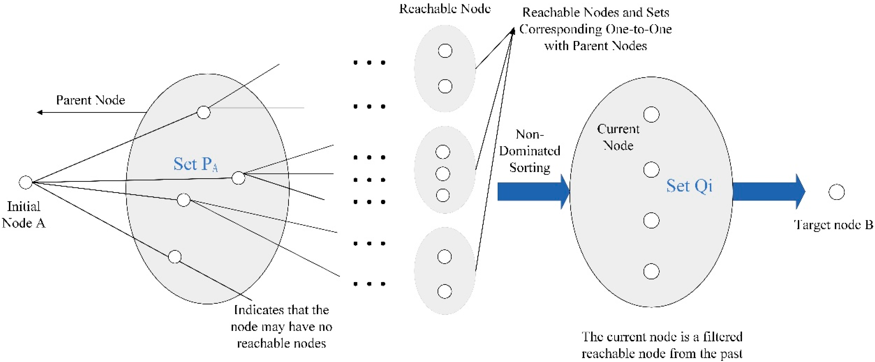
4.2. Forward Propagation Multi-Objective Path Planning Algorithm

4.2.1. Core Algorithmic Ideas

Based on the established model and addressing the shortcomings of existing algorithms, we have independently designed a forward labeling multi-objective path planning algorithm inspired by the principles of the A* algorithm. The core ideas of the algorithm are as follows:

First, a dynamic labeling method is proposed. Labels are assigned to the current node and the next node, corresponding one-to-one with the sequence in V. The distance between the current node and the next node can be directly extracted from the distance matrix D based on their correspondence with V, avoiding redundant distance calculations and significantly improving the algorithm’s efficiency.

Second, a heuristic optimization strategy is designed. During the search for the next node, the estimated distance to the destination B is considered (the number of estimated points is unpredictable and thus not pre-considered). This ensures that the path update direction consistently points toward the destination, effectively accelerating the algorithm’s optimization speed.

Third, a non-dominated sorting method is used. The current path solutions are evaluated. If a new path solution dominates the current one and is not dominated by any other current solutions, it replaces the current path solution, and both objective values are updated. By employing a non-dominated sorting strategy, we can obtain a Pareto optimal set of path solutions.

4.2.2. Core Algorithmic Steps

• Forward Labeling Setup

Since the original problem falls under the category of multi-objective optimization, the filtered-out solutions form a non-dominated set. Consequently, node branching may occur during this process, meaning that the current node set Qi may contain one or more elements. Therefore, temporary labels Qi need to be assigned to the elements in i_m. Additionally, when using non-dominated sorting to filter reachable nodes for a specific current node, multiple mutually non-dominated reachable nodes may emerge, leading to potential branching at the reachable nodes as well. Thus, temporary labels j_n must also be assigned to the elements in Pi. The label i_m evolves continuously during the optimization process, while j_n is entirely determined by its parent node.

2.

Heuristic Optimization Strategy

Without a search direction, the optimization process would become complex and time consuming, resembling exhaustive enumeration. To enhance algorithm efficiency, we draw inspiration from the heuristic function of the A* algorithm and establish a heuristic strategy for selecting the next node from the current node, as described by Equations (43)–(45).

$$f_1=g_i+h_i$$

(43)

$$f_2=F_2={\sum }_{r\in R}{\sum }_{i\in E}{\sum }_{j\in P_i}{x}_{ij}^r$$

(44)

$$g_i={\sum }_{l=E}^i{\sum }_{r=E}{x}_{l,l+1}^r\cdot d_{l,l+1}$$

(45)

Euclidean distance is used to determine the estimated distance from the current node i to the target node B:

$$h_i=\sqrt{{\left[po{s}_x\left(B\right)-po{s}_x\left(i\right)\right]}^2+{\left[po{s}_y\left(B\right)-po{s}_y\left(i\right)\right]}^2+{\left[po{s}_z\left(B\right)-po{s}_z\left(i\right)\right]}^2}$$

(46)

where f₁ represents the heuristic distance from the initial node to the target node; g_i denotes the actual distance from the starting point A to the current node i; h_i signifies the estimated distance from the current node i to the target node B; and f₂ indicates the number of nodes included in the path from point A to the current node i.

3.

Non-Dominated Sorting Method

Non-dominated sorting methods are primary approaches for solving Pareto optimal sets. For a multi-objective optimization problem, their main idea can be summarized as follows:

If all objective values of Solution 1 are superior to those of Solution 2, then Solution 1 dominates Solution 2. In the context of this problem, this is expressed as:

$$\left\{\begin{array}{c}{f}_1^1\le f_1^2|f_2^1\le f_2^2|!\left(f_1^1=f_1^2\&\&f_2^1=f_2^2\right),\left(f_1^1,f_2^1\right)\prec \left(f_1^2,f_2^2\right)\\ f_1^1\ge f_1^2|f_2^1\ge f_2^2\Vert !\left(f_1^1=f_1^2\&\&f_2^1=f_2^2\right),\left(f_1^1,f_2^1\right)\succ \left(f_1^2,f_2^2\right)\end{array}\right.$$

(47)

Non-dominated solutions are retained, while dominated solutions are eliminated. The remaining set of mutually non-dominated solutions constitutes the optimal solution set.

Figure 6 illustrates a hierarchical, multi-objective optimization-based path planning method. The system initiates exploration from the parent node via an initial node (A), where reachability analysis identifies potential path nodes (e.g., Set P₃), some of which may be marked unreachable. During planning, non-dominated sorting evaluates multiple reachable nodes for multi-objective optimization, maintaining distinct node sets (e.g., Set Q₁). A screening mechanism then selects the current node from historically reachable nodes, ultimately constructing a reachable path set with one-to-one correspondence to the parent node. This process iteratively advances toward the target node (B). The proposed structure ensures systematic path exploration while optimization algorithms guarantee path quality.

This algorithm draws inspiration from the A* algorithm’s concept of setting open and closed sets, as well as its heuristic optimization approach, and incorporates strategies such as forward labeling and non-dominated sorting. The specific steps of the algorithm are as follows.

As mentioned above, the optimal solution obtained using Algorithm 1 is within a set of Pareto optimal solutions. Therefore, it is necessary to find a strategy to select the best compromise solution from the Pareto optimal solutions.

Algorithm 1: Multi-objective path planning algorithm based on forward labels
Input:	Start point s and the target point t. Directed graph G, distance matrix D.
Output:	A set of Pareto optimal paths from s to t.
Step 1:	Initialize a label set L(v) for each vertex v ∈ V. Each label l ∈ L(v) represents a partial path from ss to vv and stores the following: The cost vector c(l) (e.g., F1, F2, and F3). The predecessor vertex p(l) to reconstruct the path.
Step 2:	Add an initial label l0 to L(s) with zero cost and no predecessor.
Step 3:	For each vertex u ∈ V in topological order (or using a priority queue) For each outgoing edge (u,v) ∈ E For each label l ∈ L(u) Create a new label l′ for vertex v. Update the cost vector: c(l′) = c(l)+Du,v. Set the predecessor: p(l′) = u. Add l′ to L(v) if it is not dominated by any existing label. Remove any labels in L(v) that are dominated by l′.
Step 4	A label l1 dominates another label l2 if c(l1) is better than or equal to c(l2) in all objectives and strictly better in at least one objective.
Step 5:	Only non-dominated labels are kept in L(v)L(v) to ensure Pareto optimality.
Step 6:	The algorithm terminates when all vertices have been processed and no further labels can be propagated.
Step 7:	The set of labels L(t) at the target vertex tt represents the Pareto optimal paths from s to t.
Step 8:	For each label l ∈ L(t), reconstruct the path by backtracking through the predecessors p(l) until reaching the start vertex s.

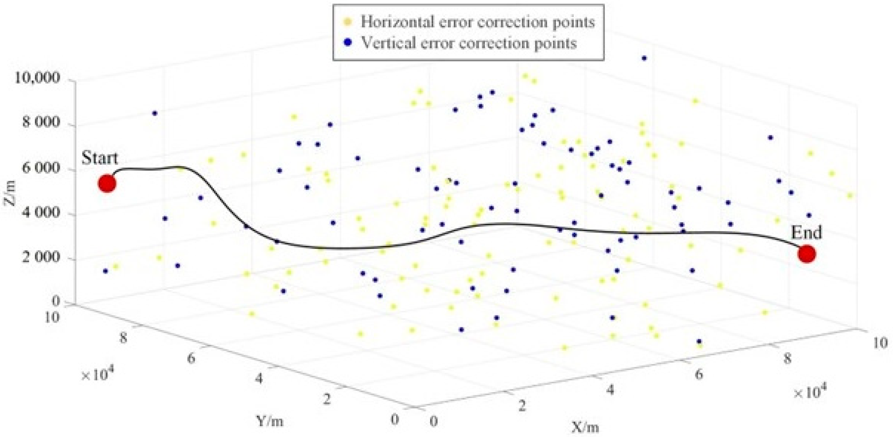
Let F_c^min, Fcmax and Fcmin, F_c^max represent the minimum and maximum values of the objective functions F1, F2, and F3 in the Pareto solution set, respectively. A membership function is established, and the satisfaction degree γ_c,_k of the objective function cc for the k-th solution in the Pareto optimal solution set is defined as

$${\gamma }_{c,k}=\left\{\begin{array}{c}1F_{c,k}\le F_c^{\mathrm{m}\mathrm{i}\mathrm{n}}\\ {\displaystyle \frac{F_c^{\mathrm{m}\mathrm{a}\mathrm{x}}-F_{c,k}}{F_c^{\mathrm{m}\mathrm{a}\mathrm{x}}-F_c^{\mathrm{m}\mathrm{i}\mathrm{n}}}}{F}_c^{\mathrm{m}\mathrm{i}\mathrm{n}}<F_{c,k}<F_c^{\mathrm{m}\mathrm{a}\mathrm{x}}\\ 0F_{c,k}\ge F_c^{\mathrm{m}\mathrm{a}\mathrm{x}}\end{array}\right.$$

(48)

And then, the satisfaction degree of the k-th solution in the Pareto optimal solution set is obtained by integrating and normalizing the satisfaction degrees as follows:

$${\gamma }_k={\displaystyle \frac{\sum _{c=1}^2{\gamma }_{c,k}}{\sum _{k=1}^K\sum _{c=1}^2{\gamma }_{c,k}}}$$

(49)

where K represents the number of elements in the Pareto optimal solution set.

The solution with the highest satisfaction degree is selected as the best compromise solution.

5. Case Studies

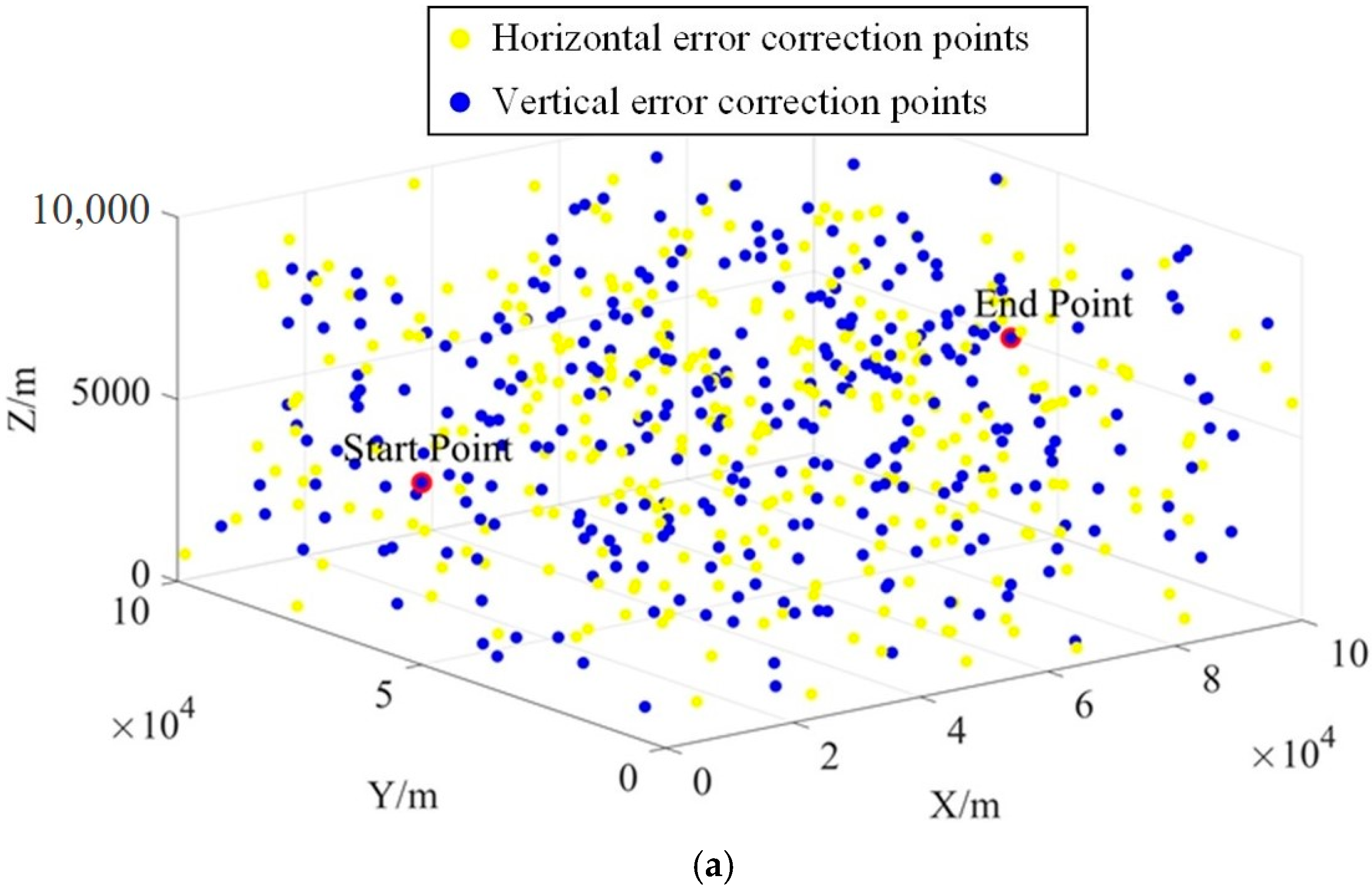
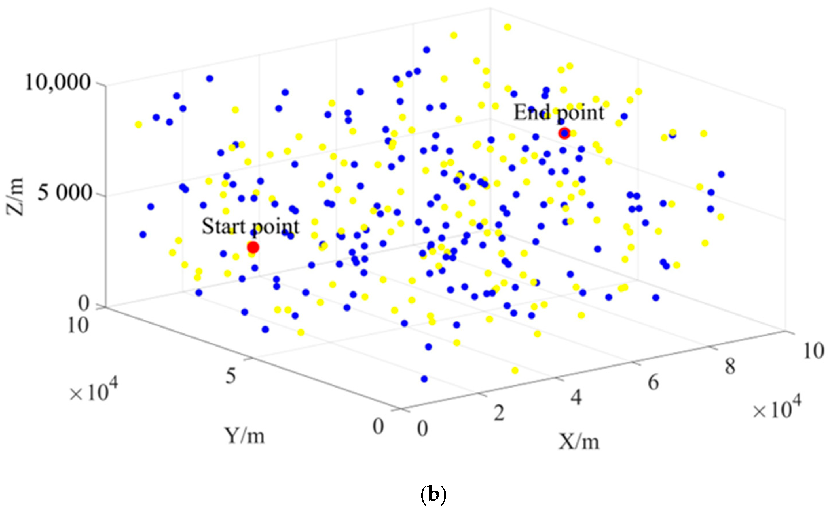
5.1. Definition of Cases

In this paper, we evaluated the proposed algorithm using two case studies, both conducted within a three-dimensional spatial region of size 10⁴ × 10⁴ ×10⁴. The distributions of correction points, start points, and end points for the two cases are illustrated in Figure 7a,b, respectively. In the figures, yellow points represent horizontal error correction points, while blue points denote vertical error correction points. Moreover, the parameters involved in the model calculation are listed in

Table 2. The main parameters involved in the objective model.

Parameters	Symbols	Value
Vertical error limitation with vertical error can be corrected (dm)	α1	25/20
Horizontal error limitation with vertical error can be corrected (dm)	α2	15/10
Vertical error limitation with horizontal error can be corrected (dm)	β1	20/15
Horizontal error limitation with horizontal error can be corrected (dm)	β2	25/20
Vertical and horizontal error increments of the UAV	δ	0.001
Minimum turning radius of the UAV (m)	M	200

, and “data/data 2” refer to the parameter values for case 1 and case 2, respectively.

5.2. Results and Discussion

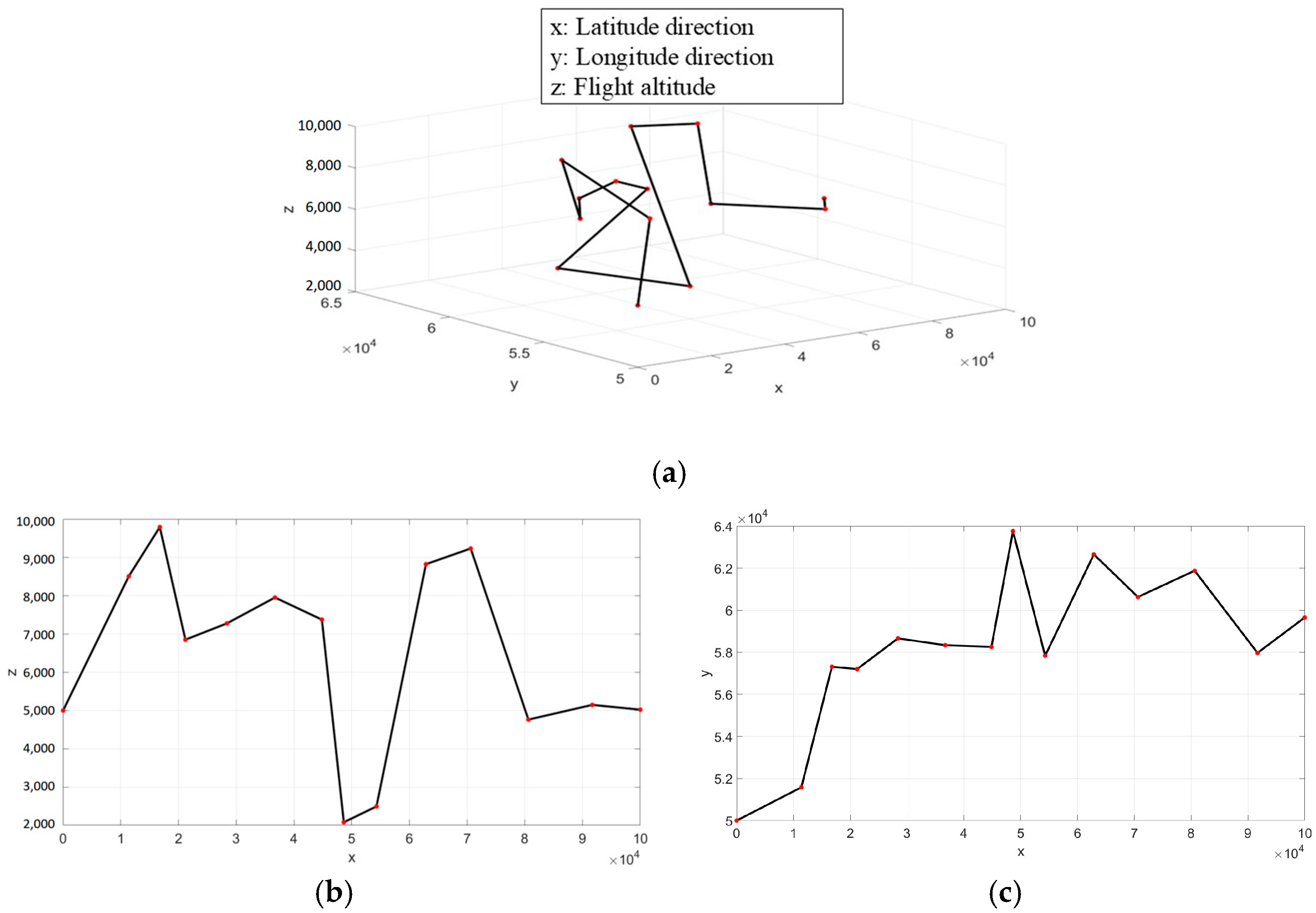
5.2.1. Results of Case 1

The proposed algorithm was applied to Case 1, and the resulting planned path is illustrated in Figure 8a–c, which includes a 3D schematic diagram and its corresponding 2D planar projections. The planned trajectory consists of the start point (Point A), the end point (Point B), and 12 intermediate correction points. The total length of the planned trajectory is 116,861 m.

To further validate the effectiveness of our proposed algorithm, we conducted comparative experiments using NSGA-II on the same case study. While NSGA-II solutions also satisfy the positioning error constraints, they require 18 correction points and yield a longer path length of 119,983 m. This demonstrates that our approach achieves approximately 2.6% reduction in total flight distance relative to NSGA-II, while maintaining equivalent positioning accuracy.

Detailed trajectory information is provided in

Table 3. Optimization results for the UAV path in Case 1.

Serial Number	Calibration Point Number	Vertical Error Before Calibration	Horizontal Error Before Calibration	Calibration Point Type
1	0	0	0	Start point
2	578	12.0107	12.0107	Horizontal
3	417	19.9754	7.9646	Vertical
4	294	5.3257	13.2903	Horizontal
5	91	12.6804	7.3547	Vertical
6	607	8.3530	15.7077	Horizontal
7	61	16.5063	8.1533	Vertical
8	193	8.5267	16.6800	Horizontal
9	375	16.7278	8.2011	Vertical
10	315	11.6958	19.8969	Horizontal
11	403	19.7218	8.0260	Vertical
12	248	11.0198	19.0458	Horizontal
13	501	22.7595	11.7397	Vertical
14	612	8.4900	20.2297	End point

, which includes the following for each segment of the path. The results demonstrate that the proposed method successfully plans a feasible path for the maritime UAV, ensuring its safe arrival at the target destination. Additionally, the method effectively reduces the total travel distance, optimizing the trajectory for efficiency and reliability.

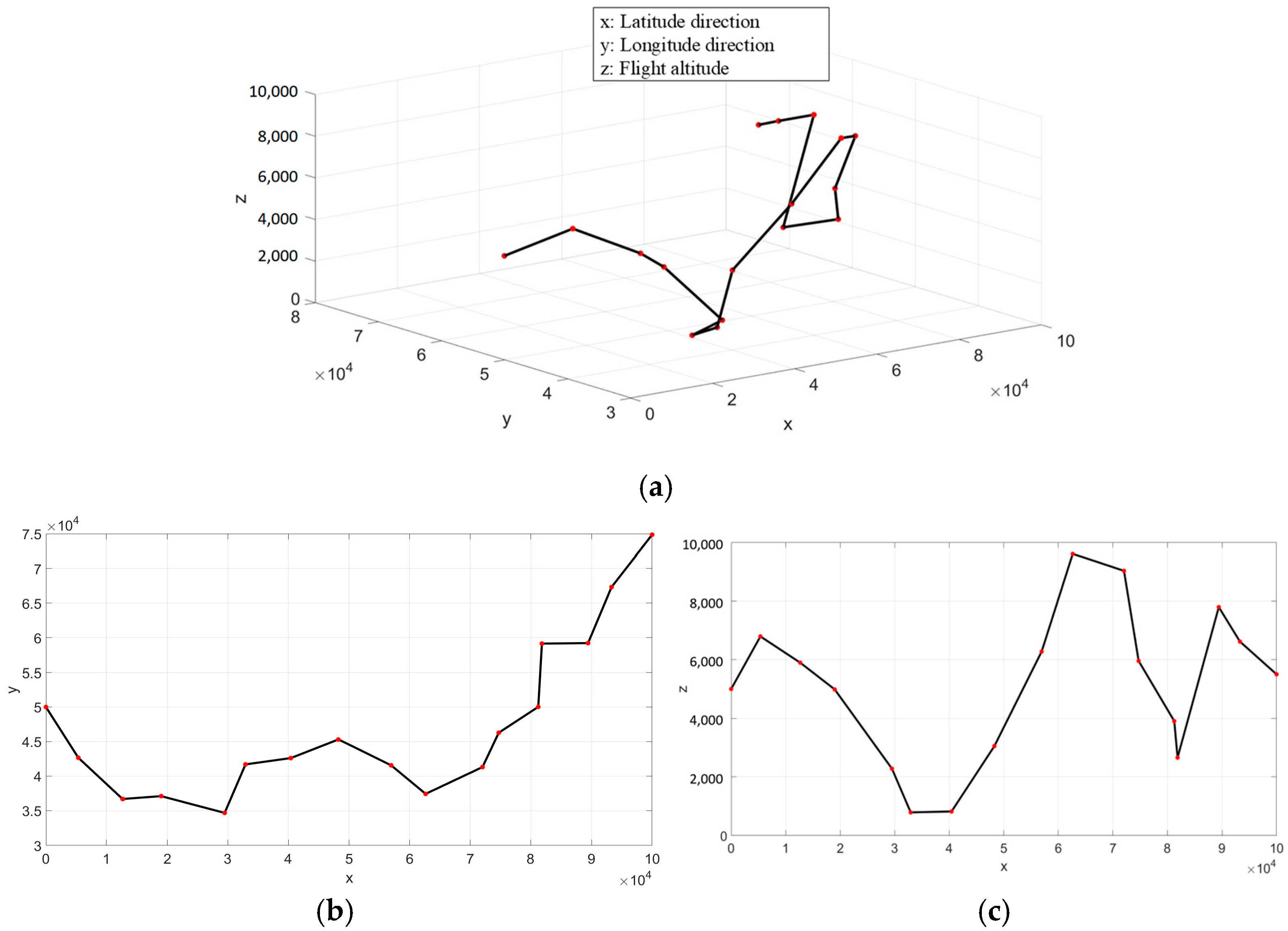
5.2.2. Results of Case 2

The proposed algorithm was applied to Case 2, and the resulting planned path is illustrated in Figure 9a–c, which includes a 3D schematic diagram and its corresponding 2D planar projections. The planned trajectory consists of the start point (Point A), the end point (Point B), and 15 intermediate correction points. The total length of the planned trajectory is 140,131 m. While NSGA-II solutions also satisfy the positioning error constraints, they require 18 correction points and yield a longer path length of 142,227 m. This demonstrates that our approach achieves approximately 1.5% reduction in total flight distance relative to NSGA-II, while maintaining equivalent positioning accuracy.

The detailed trajectory information is provided in

Table 4. Optimization results for the UAV path in Case 2.

Serial Number	Calibration Point Number	Vertical Error Before Calibration	Horizontal Error Before Calibration	Calibration Point Type
1	0	0	0	Start point
2	169	9.2705	9.2705	Horizontal
3	266	18.7485	9.4780	Vertical
4	270	6.4000	15.8780	Horizontal
5	248	17.5027	11.1027	Vertical
6	194	7.9676	19.0703	Horizontal
7	205	15.5098	7.5422	Vertical
8	108	8.5901	16.1323	Horizontal
9	73	18.5680	9.9779	Vertical
10	319	7.7937	17.7716	Horizontal
11	274	17.9803	10.1866	Vertical
12	12	6.4367	16.6233	Horizontal
13	216	14.2391	7.8024	Vertical
14	279	9.2184	17.0208	Horizontal
15	302	18.3551	9.1368	Vertical
16	161	9.0811	18.2179	Horizontal
17	326	19.2275	10.1464	End point

, which includes the following for each segment of the path.

5.2.3. Results Discussion

Conventional path planning methods developed for GPS-equipped UAVs are not directly applicable to maritime UAVs relying on INS. The direct application of such traditional approaches would inevitably lead to excessive accumulated errors in the INS, potentially resulting in UAV loss. Through two case studies, this study has demonstrated that the proposed method can effectively constrain positioning errors within the allowable threshold of 2.5 m in both vertical and horizontal directions, thereby validating its effectiveness.

6. Conclusions

This paper addresses the problem of rapid trajectory planning for aircraft in complex environments. By analyzing the motion state of the aircraft, we consider multiple objectives, including minimizing the trajectory length, reducing the number of error corrections, and maximizing the probability of reaching the destination. The proposed approach integrates knowledge from graph theory, control systems, machine learning, and probability theory to establish a multi-objective path planning algorithm. This algorithm is implemented to achieve fast trajectory planning under given start and destination conditions.

References

1. Yang, Z.; Yu, X.; Dedman, S.; Rosso, M.; Zhu, J.; Yang, J.; Xia, Y.; Tian, Y.; Zhang, G.; Wang, J. UAV remote sensing applications in marine monitoring: Knowledge visualization and review. Sci. Total Environ. 2022, 838, 155939. [Google Scholar] [CrossRef] [PubMed]
2. Ma, D.; Ma, W.; Jin, S.; Ma, X. Method for simultaneously optimizing ship route and speed with emission control areas. Ocean Eng. 2020, 202, 107170. [Google Scholar] [CrossRef]
3. Ventura, D.; Bonifazi, A.; Gravina, M.F.; Belluscio, A.; Ardizzone, G. Mapping and classification of ecologically sensitive marine habitats using unmanned aerial vehicle (UAV) imagery and object-based image analysis (OBIA). Remote Sens. 2018, 10, 1331. [Google Scholar] [CrossRef]
4. Nomikos, N.; Gkonis, P.K.; Bithas, P.S.; Trakadas, P. A survey on UAV-aided maritime communications: Deployment considerations, applications, and future challenges. IEEE Open J. Commun. Soc. 2022, 4, 56–78. [Google Scholar] [CrossRef]
5. Wang, X.; Yang, L.T.; Meng, D.; Dong, M.; Ota, K.; Wang, H. Multi-UAV cooperative localization for marine targets based on weighted subspace fitting in SAGIN environment. IEEE Internet Things J. 2021, 9, 5708–5718. [Google Scholar] [CrossRef]
6. Taddia, Y.; Corbau, C.; Buoninsegni, J.; Simeoni, U.; Pellegrinelli, A. UAV approach for detecting plastic marine debris on the beach: A case study in the Po River Delta (Italy). Drones 2021, 5, 140. [Google Scholar] [CrossRef]
7. Dujon, A.M.; Ierodiaconou, D.; Geeson, J.J.; Arnould, J.P.Y.; Allan, B.M.; Katselidis, K.A.; Schofield, G. Machine learning to detect marine animals in UAV imagery: Effect of morphology, spacing, behaviour and habitat. Remote Sens. Ecol. Conserv. 2021, 7, 341–354. [Google Scholar] [CrossRef]
8. Ma, W.; Lu, T.; Ma, D.; Wang, D. Ship route and speed multi-objective optimization considering weather conditions and emission control area regulations. Marit. Policy Manag. 2021, 48, 1053–1068. [Google Scholar] [CrossRef]
9. Ma, W.; Ma, D.; Ma, Y.; Zhang, J.; Wang, D. Green maritime: A routing and speed multi-objective optimization strategy. J. Clean. Prod. 2021, 305, 127179. [Google Scholar] [CrossRef]
10. Ma, W.; Han, Y.; Tang, H.; Ma, D.; Zheng, H.; Zhang, Y. Ship route planning based on intelligent mapping swarm optimization. Comput. Ind. Eng. 2023, 176, 108920. [Google Scholar] [CrossRef]
11. Blasi, L.; D’Amato, E.; Mattei, M.; Notaro, I. UAV path planning in 3-d constrained environments based on layered essential visibility graphs. IEEE Trans. Aerosp. Electron. Syst. 2022, 59, 2359–2375. [Google Scholar] [CrossRef]
12. Yan, F.; Liu, Y.S.; Xiao, J.Z. Path planning in complex 3D environments using a probabilistic roadmap method. Int. J. Autom. Comput. 2013, 10, 525–533. [Google Scholar] [CrossRef]
13. Mokrane, A.; BRAHAM, A.C.; Cherki, B. UAV path planning based on dynamic programming algorithm on photogrammetric DEMs. In Proceedings of the 2020 International Conference on Electrical Engineering (ICEE), Istanbul, Turkey, 25–27 September 2020; pp. 1–5. [Google Scholar]
14. Bauso, D.; Giarré, L.; Pesenti, R. Multiple UAV cooperative path planning via neuro-dynamic programming. In Proceedings of the 2004 43rd IEEE Conference on Decision and Control (CDC) (IEEE Cat. No. 04CH37601), Nassau, Bahamas, 14–17 December 2004; Volume 1, pp. 1087–1092. [Google Scholar]
15. Radmanesh, M.; Kumar, M. Flight formation of UAVs in presence of moving obstacles using fast-dynamic mixed integer linear programming. Aerosp. Sci. Technol. 2016, 50, 149–160. [Google Scholar] [CrossRef]
16. Tu, B.; Wang, F.; Han, X. 3D path planning for UAV based on a hybrid algorithm of marine predators algorithm with quasi-oppositional learning and differential evolution. Egypt. Inform. J. 2024, 28, 100556. [Google Scholar] [CrossRef]
17. Wang, G.G.; Cai, X.; Cui, Z.; Min, G.; Chen, J. High performance computing for cyber physical social systems by using evolutionary multi-objective optimization algorithm. IEEE Trans. Emerg. Top. Comput. 2017, 8, 20–30. [Google Scholar] [CrossRef]
18. Bayili, S.; Polat, F. Limited-Damage A*: A path search algorithm that considers damage as a feasibility criterion. Knowl.-Based Syst. 2011, 24, 501–512. [Google Scholar] [CrossRef]
19. Chen, J.; Li, M.; Yuan, Z.; Gu, Q. An improved A* algorithm for UAV path planning problems. In Proceedings of the 2020 IEEE 4th Information Technology, Networking, Electronic and Automation Control Conference (ITNEC), Chongqing, China, 12–14 June 2020; Volume 1, pp. 958–962. [Google Scholar]
20. Meng, B. UAV path planning based on bidirectional sparse A* search algorithm. In Proceedings of the 2010 International Conference on Intelligent Computation Technology and Automation, Changsha, China, 11–12 May 2010; Volume 3, pp. 1106–1109. [Google Scholar]
21. Aslan, S. Back-and-Forth (BaF): A new greedy algorithm for geometric path planning of unmanned aerial vehicles. Computing 2024, 106, 2811–2849. [Google Scholar] [CrossRef]
22. Ma, W.; Zhang, J.; Han, Y.; Zheng, H.; Ma, D.; Chen, M. A chaos-coupled multi-objective scheduling decision method for liner shipping based on the NSGA-III algorithm. Comput. Ind. Eng. 2022, 174, 108732. [Google Scholar] [CrossRef]
23. Duan, H.; Yu, Y.; Zhang, X.; Shao, S. Three-dimension path planning for UCAV using hybrid meta-heuristic ACO-DE algorithm. Simul. Model. Pract. Theory 2010, 18, 1104–1115. [Google Scholar] [CrossRef]
24. Zhao, B.; Huo, M.; Li, Z.; Yu, Z.; Qi, N. Clustering-based hyper-heuristic algorithm for multi-region coverage path planning of heterogeneous UAVs. Neurocomputing 2024, 610, 128528. [Google Scholar] [CrossRef]
25. Wu, S.; He, B.; Zhang, J.; Chen, C.; Yang, J. PSAO: An enhanced Aquila Optimizer with particle swarm mechanism for engineering design and UAV path planning problems. Alex. Eng. J. 2024, 106, 474–504. [Google Scholar] [CrossRef]
26. Li, L.; Gu, Q.; Liu, L. Research on path planning algorithm for multi-UAV maritime targets search based on genetic algorithm. In Proceedings of the 2020 IEEE International Conference on Information Technology, Big Data and Artificial Intelligence (ICIBA), Chongqing, China, 6–8 November 2020; Volume 1, pp. 840–843. [Google Scholar]
27. Boulares, M.; Barnawi, A. A novel UAV path planning algorithm to search for floating objects on the ocean surface based on object’s trajectory prediction by regression. Robot. Auton. Syst. 2021, 135, 103673. [Google Scholar] [CrossRef]
28. Boulares, M.; Fehri, A.; Jemni, M. UAV path planning algorithm based on Deep Q-Learning to search for a floating lost target in the ocean. Robot. Auton. Syst. 2024, 179, 104730. [Google Scholar] [CrossRef]
29. He, L.; Aouf, N.; Song, B. Explainable Deep Reinforcement Learning for UAV autonomous path planning. Aerosp. Sci. Technol. 2021, 118, 107052. [Google Scholar] [CrossRef]
Figure 1. Schematic diagram of a UAV’s shortest path and the positioning error correction path.
Jmse 13 00870 g001
Figure 2. Path planning scenario for maritime UAVs across multiple positioning points.
Jmse 13 00870 g002
Figure 3. A directed graph for UAVs path planning with 24 nodes.
Jmse 13 00870 g003
Figure 4. Schematic diagram of Dubins path for UAVs.
Jmse 13 00870 g004
Figure 5. Schematic diagram of 3D trajectory plane unfolding.
Jmse 13 00870 g005
Figure 6. Search process of the forward labeling algorithm.
Jmse 13 00870 g006
Figure 7. Distribution of correction points, start points, and end points: (a) case 1; (b) case 2.
Jmse 13 00870 g007aJmse 13 00870 g007b
Figure 8. Optimized path for the UAV in Case 1: (a) 3D perspective; (b) XOZ perspective; and (c) XOY perspective.
Jmse 13 00870 g008
Figure 9. Optimized path for the UAV in Case 2: (a) 3D perspective; (b) XOZ perspective; and (c) XOY perspective.
Jmse 13 00870 g009