Compression of Marine Environmental Data Using Convolutional Attention Autoencoder

Abstract

Ocean temperature data is fundamental to the study of ocean dynamics and climate change, and its efficient compression and storage are critical for large-scale data analysis and transmission. However, traditional compression methods based on Fourier transform struggle to balance compression ratio and fidelity when confronted with the complex characteristics of marine environments. This study proposes a convolutional attention autoencoder (CAAE) to compress and reconstruct three-dimensional temperature fields and evaluates its performance across different depths and compression ratios. The experimental results indicate that although reconstruction error slightly increases with higher compression ratios, the proposed model achieves near-perfect compression and reconstruction of marine environmental data, performing robustly across various depths and spatial locations. This work offers a viable solution for the efficient and accurate compression of three-dimensional ocean data and provides valuable insights for the management of large-scale marine datasets.

1. Introduction

With the continuous enhancement of global marine exploration and utilization, marine environmental data have become indispensable in numerous fields such as ship navigation, offshore construction, maritime search and rescue, marine resource exploration and development, and marine ecological protection [1,2]. Such data are characterized by multidimensionality, multiple scales, and diverse types—including sea surface temperature, three-dimensional temperature fields, salinity fields, ocean current fields, wave data, and seafloor topography [3]. These datasets are highly interrelated and coupled, and their volumes are often enormous (e.g., high-resolution marine remote sensing imagery, underwater detection data, and seafloor acoustic data) [4]. The overall data volume is rapidly expanding to terabyte or even petabyte scales. For vessels engaged in maritime operations, the real-time or near-real-time acquisition of marine environmental data is critical for route planning, risk assessment, and ensuring operational safety. However, satellite communication links, on which vessels depend, are limited in bandwidth and stability, making it challenging to meet the demands of long-duration, high-speed transmission of massive data volumes [5]. Therefore, achieving efficient compression and transmission of massive marine environmental data within a limited bandwidth environment holds significant engineering and societal value [6].

Traditional data compression methods—such as lossy or lossless techniques based on wavelets, wavelet packets, and discrete cosine transforms—have achieved favorable results in image processing, video compression, and the compression of certain spatiotemporal datasets. For example, multi-resolution analysis based on Fourier or wavelet transforms can effectively compress spatiotemporal distribution data from oceanic meteorological and wave fields [7]. However, these conventional methods often struggle to balance high compression ratios with high fidelity when handling three-dimensional or multi-source heterogeneous marine data (e.g., high-resolution underwater topography derived from multiple sensors) [8]. Furthermore, as the precision and frequency of marine observations improve, the intrinsic structure of massive datasets becomes increasingly complex. Traditional feature extraction and encoding methods may fail to capture critical fine-scale features, resulting in reconstructed data that do not meet the requirements for marine monitoring, forecasting, and decision-making [9].

In recent years, the rapid development of deep learning theories and algorithms has led to the emergence of models such as autoencoders, convolutional neural networks (CNNs), recurrent neural networks (RNNs), and generative adversarial networks (GANs), which demonstrate tremendous potential in feature extraction and representation learning, thereby offering new approaches for compressing high-dimensional data [10,11]. The advantage of deep learning methods in data compression lies in their ability to learn low-dimensional representations that effectively capture data distributions via end-to-end training on large-scale datasets. This approach maps redundant information into a compact latent space, achieving high compression ratios without compromising reconstruction accuracy [12].

Early applications of deep learning in data compression focused primarily on image compression, while its application to scientific data compression has only recently begun to emerge [13]. For instance, Liu et al. employed GANs to compress computational fluid dynamics data [14]. Although their approach introduced a novel deep learning architecture, it did not yield a significant improvement in RMSE compared to discrete wavelet transforms. Chandak et al. explored the compression of multivariate time series from IoT devices (e.g., smartwatches and sensors) by leveraging inter-variable correlations and temporal patterns. By optimizing prediction models and fine quantization, they achieved high compression ratios with excellent error control [15]. Glaws et al. utilized deep learning methods to compress in situ data from large-scale turbulence simulations, proposing an efficient end-to-end neural network model that attains high compression ratios with minimal accuracy loss [16]. However, compared to these datasets, marine environmental data possess more complex characteristics [17]. Typical marine datasets exhibit high-dimensional features (such as temperature and salinity fields) that encompass both horizontal and vertical spatial distributions as well as dynamic temporal variations [18]. Significant spatial heterogeneity and temporal correlations further complicate the task of adequately compressing and reconstructing these datasets using simple dimensionality reduction methods [19].

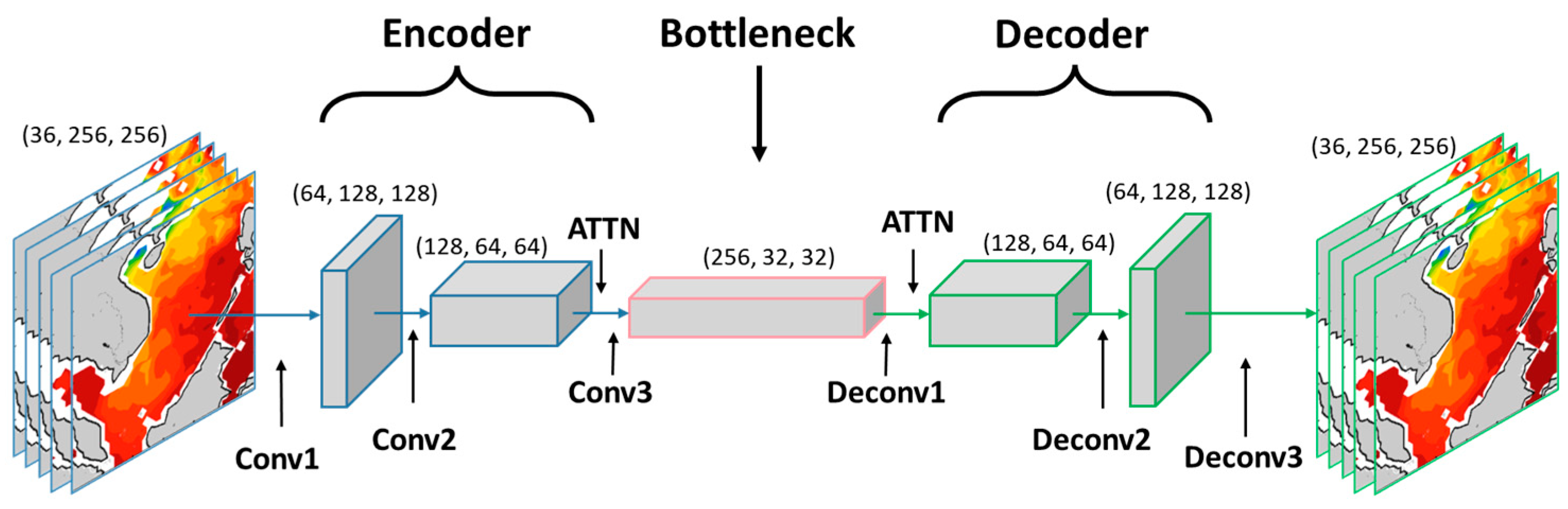
To address these challenges, this paper proposes an autoencoder model integrated with an attention mechanism to better accommodate the complex characteristics of high-dimensional marine environmental data. The model incorporates a multi-head attention mechanism into the traditional autoencoder framework to capture long-range dependencies across different spatial dimensions, temporal dimensions, and inter-variable relationships. By dynamically assigning attention weights to various regions or variables, the model can more accurately extract key features. Furthermore, a hierarchical latent space structure is designed to disentangle and represent multi-scale features, ensuring effectiveness and robustness in complex data environments.

2. Data

In this study, three-dimensional temperature fields are used to evaluate the proposed approach. The ocean temperature data were obtained from the Copernicus Marine Service (CMEMS; official website: https://marine.copernicus.eu/; accessed on 20 January 2025). Specifically, the dataset used is the Global Ocean Physics Analysis and Forecast product (Product ID: GLOBAL_ANALYSIS_FORECAST_PHY_001_024). This dataset provides high-resolution three-dimensional ocean physical fields on a global scale, including variables such as temperature, salinity, and ocean current velocity. The temperature field covers the entire water column with 36 vertical layers (ranging from 0 m to 1062 m), a horizontal resolution of 0.083° × 0.083°, and a temporal resolution of one day. The training dataset spans from 1 January 2015 to 31 December 2020, while the testing dataset covers 1 January 2021 to 31 December 2021.

3. Model

3.1. Model Architecture

A convolutional attention autoencoder model is proposed for the compression and reconstruction of marine environmental data (Figure 1). The model comprises an encoder and a decoder, which together perform dimensionality reduction on high-dimensional input data and reconstruct high-quality outputs. To enhance the extraction and reconstruction of critical spatial features, a multi-head attention mechanism is integrated into the decoder architecture. Specifically, the attention module is applied immediately after the initial transposed convolutional layer in the decoder, where the latent representation is first upscaled. This strategic placement enables the mechanism to dynamically amplify regions of the latent tensor that correspond to salient features in the original temperature field. The multi-head structure allows parallel attention to different feature subspaces, thereby preserving both fine-grained spatial details and global patterns during reconstruction. While the current implementation leverages a standard multi-head configuration optimized for the dataset’s characteristics, future studies may explore alternative attention variants to further refine feature prioritization. The encoder employs multiple Conv2D layers with progressive channel expansion to extract hierarchical features: early layers capture local spatial correlations, while deeper layers encode higher-order global patterns. The decoder uses transposed convolutions to gradually restore spatial resolution, with the attention mechanism strategically inserted to modulate the relevance of feature maps during upsampling. This design ensures that critical environmental patterns are prioritized during reconstruction, resulting in outputs that closely align with the original three-dimensional temperature field’s structural complexity.

For the input of a certain vector, its propagation in the attention layer is as follows:

The input vector is multiplied by three trainable weight matrices, W^q, W^k, and W^v, giving three attributes $Q$ (query), $K$ (key), and $V$ (value) of the vector, respectively, representing the tensor of query, the tensor of relevance between the queried information and other information, and the tensor of the information being queried. For the input vector $a_i$, the process can be represented by

$$\left\{\begin{array}{l}{q}^i=a_i{W}^q,\hfill \\ k^i=a_i{W}^k,\hfill \\ v^i=a_i{W}^v.\hfill \end{array}\right.$$

To obtain the self-attention value of any input vector, the q value of the vector is multiplied by the k value of other input vectors, and then multiplied by its v value after Softmax transformation. To prevent the disappearance of the gradient of Softmax when the input value is enormous, the value is divided by the square root, $\sqrt{d_k}$, of the dimension of the vector k before Softmax transformation. For the input vector $a_i$ and the output vector $b_i$, the process is represented by

$${\widehat{a}}_{ij}=soft\max \left(q^i{k}^j/\sqrt{d_k}\right),$$

$$b_i={\displaystyle \sum {\widehat{a}}_{ij}{v}^j}.$$

Furthermore, we use the multi-head self-attention mechanism, in which the input vector is divided into $h$ parts, where $h$ is the number of attention heads, and is transferred to each attention head. Then, the calculation results of each attention head are spliced, and a trainable weight matrix $W^o$ is introduced to multiply the concatenated matrix. This process can be represented as:

$$\mathrm{MultiHead}(Q,K,V)=\mathrm{Concat}(hea{d}_1,\dots ,hea{d}_n)W^o.$$

The specific number of layers and architecture of the encoder and decoder can be adjusted according to the compression requirements, thereby accommodating varying levels of data complexity and target compression ratios. For example, the dimensionality of the latent space can be selected to meet the desired compression rate, and the depth of the encoder/decoder can be tuned to balance the precision of feature extraction and reconstruction. During training, the model is optimized end-to-end using the mean squared error (MSE) loss function to quantify the difference between the original and reconstructed data, ensuring high efficiency and accuracy in both the compression and decompression stages.

3.2. Evaluation Metrics

To accurately assess the model’s performance, two commonly used metrics are employed: mean absolute error (MAE) and mean absolute percentage error (MAPE). These metrics are defined as follows

$$MAPE=\frac{1}{n}\sum _{i=1}^n\left|\frac{{\hat{y}}_i-y_i}{y_i}\right|$$

$$MAE=\frac{1}{n}\sum _{i=1}^n|{\hat{y}}_i-y_i|$$

where $\hat{y}$ denotes the reconstructed value, y the actual value, and n the number of samples. A lower MAE indicates a higher reconstruction accuracy, while a lower MAPE, which is sensitive to relative errors, indicates higher predictive precision.

4. Experiments and Results

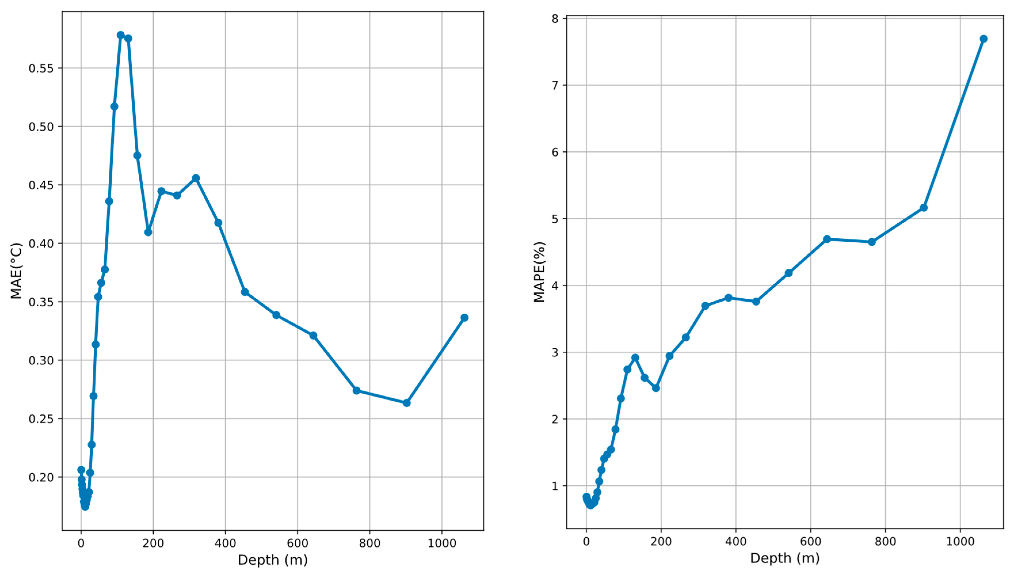
Figure 2 shows the variation of root-mean-square error (RMSE) and MAPE with depth for South China Sea temperature data during the compression and reconstruction process at a compression ratio of 18.

In the shallow water region (0–200 m), RMSE increases rapidly, peaking near 50 m at approximately 0.55 °C (Figure 2, left panel). This is attributed to the significant influence of external environmental factors in shallow waters, such as strong sea surface temperature fluctuations caused by wind stress, solar radiation, and coastal dynamic processes (e.g., upwelling and eddies). These complex and nonlinear dynamics render compression and reconstruction more challenging, thereby causing a notable increase in RMSE. In addition, because the absolute temperature values in the shallow region are relatively high, the impact on MAPE is comparatively muted, resulting in a relatively low and stable MAPE (ranging from 1% to 4%; Figure 2, right panel).

In the intermediate layer (200–600 m), RMSE gradually decreases and stabilizes around 400 m, maintaining values between 0.35 °C and 0.40 °C. This trend reflects the relatively stable temperature field in this region. Compared to the highly dynamic shallow layers, the intermediate region is less affected by deep ocean dynamics and exhibits weaker temperature gradients, enabling the compression model to more accurately reconstruct temperature features. However, within this depth range, MAPE shows a gradual increase, likely due to the lower absolute temperature values. With stable absolute errors, the percentage error (MAPE) becomes more sensitive to these lower temperatures, resulting in a continuous increase.

In the deep layers (600–1000 m), the root-mean-square error (RMSE) further decreases, reaching a minimum of approximately 0.25 °C between 600 m and 800 m (Figure 2, left panel). While reconstruction errors in deep-sea temperatures are significantly lower than in shallower layers, it is important to note that this reduced error is largely attributable to the inherently low natural variability of deep-sea temperatures. As depth increases, the mean absolute percentage error (MAPE) exhibits a pronounced upward trend, peaking at approximately 8% at 1000 m (Figure 2, right panel). This increase is primarily driven by the extremely low absolute temperature values in deep layers (near freezing); although the absolute error decreases with depth, the relative error metric (MAPE) becomes disproportionately sensitive to small baseline temperatures. Furthermore, the subtle natural variations in deep-sea temperature data may limit the model’s capacity to resolve minor temperature gradients or local features, resulting in suboptimal reconstruction performance under conditions of extreme low-temperature stability.

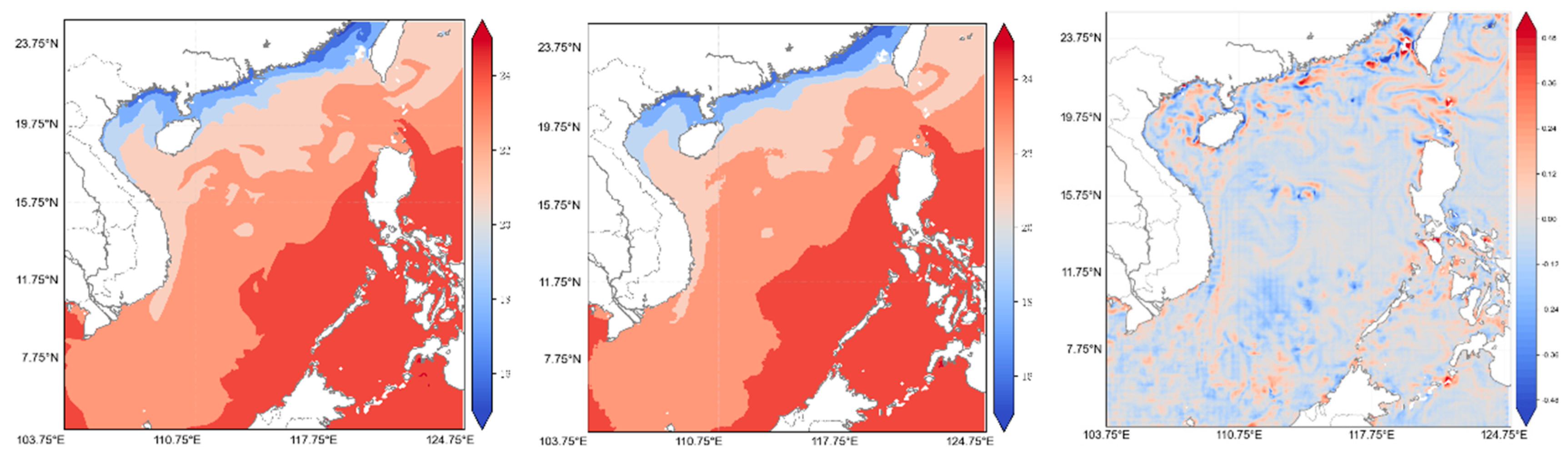
To further illustrate the differences in temperature distribution before and after reconstruction, Figure 3, Figure 4 and Figure 5 present comparisons for the South China Sea at the sea surface (SST), 100 m, and 200 m depths, respectively. These figures also show the errors between the original and reconstructed data, highlighting the reconstruction accuracy. At the sea surface, the reconstructed temperature distribution aligns well with the original data across most areas. Notably, coastal regions (e.g., the Gulf of Tonkin and the southwest South China Sea) display well-reproduced temperature gradients. However, in the central deep-sea region, the reconstructed data exhibit slightly lower temperatures than the original, leading to localized discrepancies. This phenomenon may be related to the complex dynamics in the shallow region, where solar radiation, wind stress, and local eddies induce dramatic temperature variations, thereby complicating the compression and reconstruction processes.

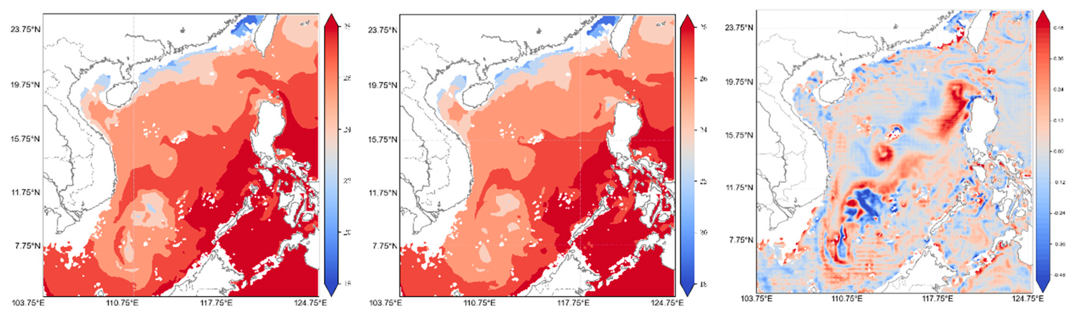
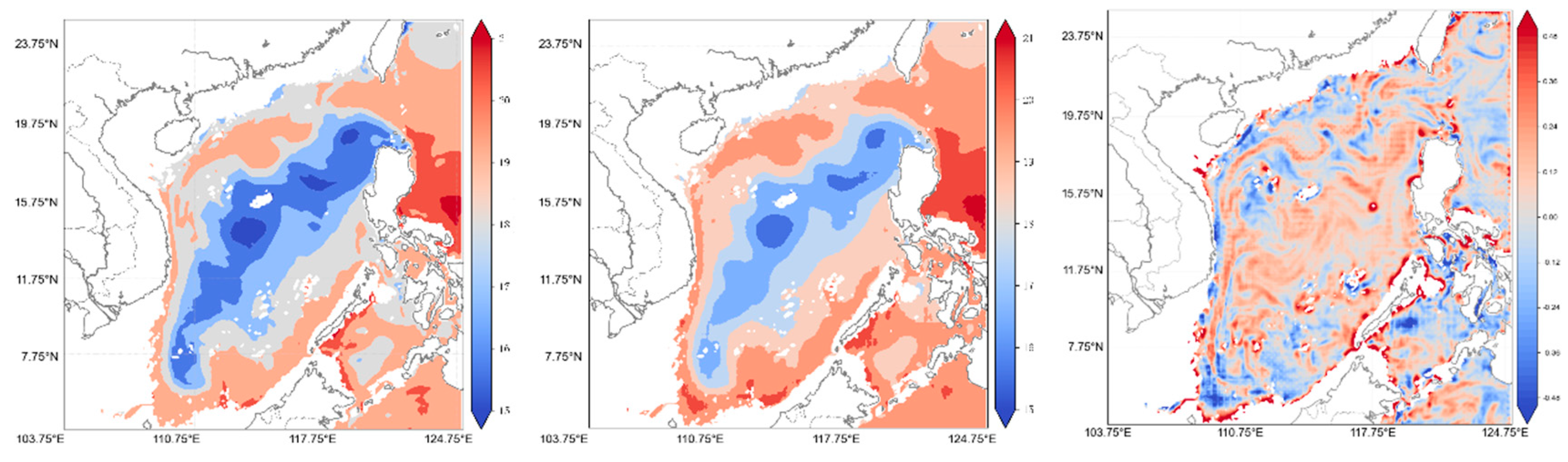
At 100 m in depth, the overall error between the reconstructed and original data is significantly reduced, and the reconstruction quality is markedly improved. At this depth, the temperature field is primarily governed by ocean currents and mesoscale eddies, which are more stable than the dynamics in shallow regions. Consequently, the model more accurately replicates the original temperature distribution, especially in the central South China Sea, where spatial gradients and feature variations are well reconstructed. Nevertheless, in some localized areas (e.g., the northeastern South China Sea), a slight underestimation is observed in the thermocline region, which may indicate some limitations of the compression model in capturing complex thermocline gradients.

At a 200 m depth, the spatial consistency between the reconstructed and original temperature distributions is further enhanced, demonstrating the model’s high precision in the compression and reconstruction of deep ocean data. The temperature field at this depth is relatively smooth with minor gradient variations compared to shallower regions, allowing for more accurate recovery of spatial features. However, in certain low-temperature regions in the central and eastern South China Sea, the reconstructed data display a slight overestimation, possibly due to the minimal temperature variations in deep-sea areas causing the model to overlook subtle gradients during compression.

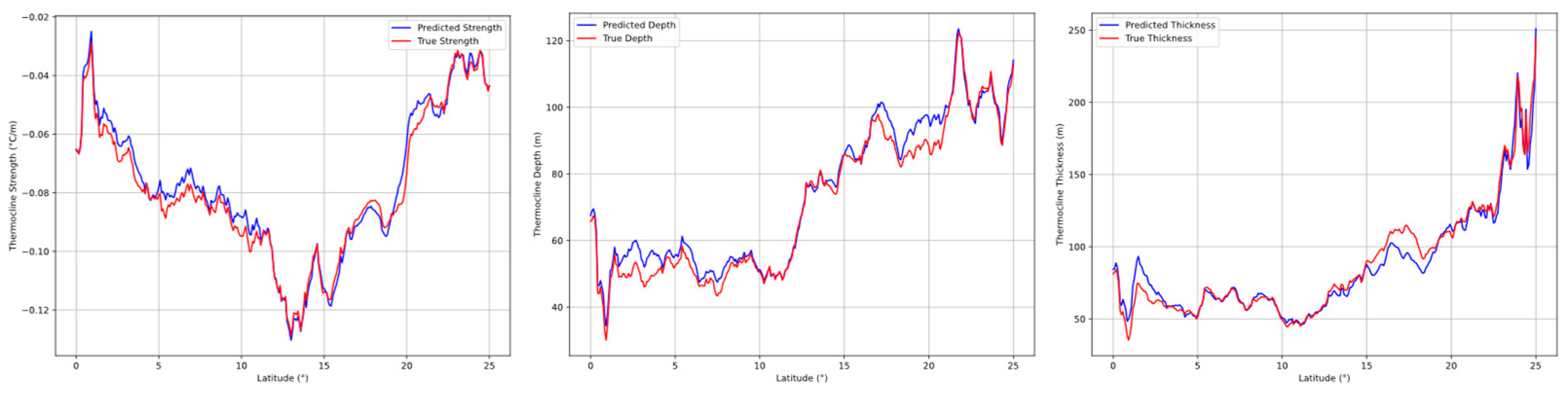
The reconstructed data’s ability to reflect the scientific features of the original data is a critical aspect in evaluating data quality [20]. We compare the thermocline characteristics (depth, strength, and thickness) identified from both the original and reconstructed datasets along latitudinal gradients (Figure 6). This evaluation assesses the preservation of key physical properties essential for understanding ocean dynamics. As illustrated in the figure, the predicted thermocline properties exhibit strong fidelity to the ground-truth curves across varying latitudes. The alignment of peak values and overall trends demonstrates that the reconstruction process effectively preserves primary oceanographic patterns. While minor discrepancies emerge in regions of rapid thermocline variability—particularly in transition zones between stable water masses—the consistency in capturing dominant features underscores the method’s capability to retain scientifically meaningful information. Notably, the preservation of critical parameters such as thermocline depth gradients and strength variations indicates that the compression–reconstruction workflow maintains sufficient resolution for rigorous analysis of vertical ocean structure and its latitudinal evolution.

To systematically examine reconstruction variations across regions with varying dynamic complexities and their seasonal influences, we analyzed temperature errors (MAE and MAPE) in three marine areas (

Table 1. Seasonal errors of reconstructed temperatures in distinct marine regions.

Area	Reconstructed MAE (°C)				Reconstructed MAPE
	Spring	Summer	Autumn	Winter	Spring	Summer	Autumn	Winter
South China Sea	0.40	0.40	0.39	0.38	2.40%	2.41%	2.32%	2.28%
East China Sea	0.42	0.42	0.46	0.44	2.37%	2.44%	2.41%	2.43%
Central Pacific	0.41	0.39	0.40	0.39	2.01%	1.95%	1.99%	1.98%

): the South China Sea (moderate complexity), East China Sea (high complexity), and Central Pacific (low complexity). The reconstructed temperature errors (MAE and MAPE) across the three regions with varying dynamic complexity show minimal seasonal fluctuations, suggesting that seasonal changes exert limited influence on model performance. In the South China Sea, MAE values remain tightly clustered between 0.38 °C (winter) and 0.40 °C (spring/summer), with MAPE varying by only 0.13% (2.28–2.41%), indicating stable reconstruction accuracy year-round. Similarly, the Central Pacific exhibits nearly constant errors, with MAE differences ≤0.02 °C (0.39–0.41 °C) and MAPE ≤ 0.06% (1.95–2.01%), underscoring the model’s robustness in regions with simpler hydrodynamic conditions. While the East China Sea, the most dynamically complex region, shows slightly larger seasonal variations (MAE: 0.42–0.46 °C; MAPE: 2.37–2.44%), these fluctuations remain modest compared to the overarching differences between the regions. Notably, the East China Sea’s highest MAE (0.46 °C in autumn) still falls within a narrow absolute range, reinforcing the fact that regional complexity, rather than seasonal dynamics, dominates error patterns.

Furthermore, the relationship between compression ratio and reconstruction error is examined across three distinct models: fast Fourier transform (FFT) [21], generative adversarial network (GAN) [14], and the proposed CAAE (

Table 2. Error comparison under different compression ratios.

Original Size	Compressed Size	Compression Ratio	Reconstructed MAE (°C)			Reconstructed MAPE
			FFT	GAN	CAAE	FFT	GAN	CAAE
531.7 MB	14.7 MB	36.2	1.76	0.65	0.56	8.41%	3.54%	3.31%
531.7 MB	29.5 MB	18.0	1.52	0.43	0.38	7.36%	2.40%	2.28%
531.7 MB	59.6 MB	8.9	1.34	0.32	0.29	6.65%	1.93%	1.82%
531.7 MB	118.3 MB	4.5	1.15	0.18	0.18	5.8%	1.16%	1.18%

). The comparison reveals significant differences in reconstruction accuracy under varying compression ratios. At the highest compression ratio (36.2), the proposed CAAE achieves superior performance with a reconstructed MAE of 0.56 °C and MAPE of 3.31%, outperforming both GAN (MAE: 0.65 °C, MAPE: 3.54%) and FFT (MAE: 1.76 °C, MAPE: 8.41%). This demonstrates that CAAE preserves critical data features more effectively under aggressive compression, mitigating the trade-off between space efficiency and fidelity. The advantage of CAAE persists across intermediate compression ratios. For instance, at a ratio of 18.0, CAAE reduces MAE by 11.6% compared to GAN (0.38 °C vs. 0.43 °C) and MAPE by 5.0% (2.28% vs. 2.40%), while FFT remains significantly less accurate (MAE: 1.52 °C, MAPE: 7.36%). Notably, at the lowest compression ratio (4.5), CAAE matches GAN in MAE (0.18 °C) and slightly exceeds it in MAPE (1.18% vs. 1.16%), suggesting comparable feature retention capabilities when latent space constraints are relaxed.

The inverse relationship between compression ratio and reconstruction error remains consistent across all the models. For CAAE, reducing the compression ratio from 36.2 to 4.5 improves MAE by 67.9% (0.56 °C to 0.18 °C) and MAPE by 64.3% (3.31% to 1.18%), confirming that lower ratios expand the latent space for capturing fine-grained thermal patterns. However, this improvement comes at a storage cost: compressed data size increases from 14.7 MB to 118.3 MB (20% of the original volume), mirroring trends in GAN and FFT. Thus, while CAAE optimizes the accuracy-space trade-off, the fundamental compromise persists; high compression sacrifices granular details, whereas low compression prioritizes fidelity at the expense of practicality for storage-limited applications.

In practical terms, CAAE expands the viable design space for compression systems. For scenarios requiring extreme compression (e.g., satellite telemetry), CAAE’s high-ratio performance (MAE: 0.56at a compression ratio of 36.2 makes it preferable to FFT’s error-prone reconstructions or GAN’s intermediate results. Conversely, for high-precision applications like climate modeling, CAAE’s low-ratio mode (0.18 °C MAE) offers accuracy comparable to GAN while maintaining architectural simplicity. This dual capability positions CAAE as a versatile framework adaptable to diverse operational constraints.

5. Conclusions

This study investigated the compression and reconstruction of three-dimensional temperature field data from the South China Sea using a convolutional autoencoder model integrated with an attention mechanism. The results indicate that the model performs exceptionally well in deep-sea regions, where reconstruction errors are significantly lower compared to shallow regions—consistent with the relatively stable temperature distributions found at depth. In contrast, the shallow regions exhibit higher errors due to the influence of complex dynamic processes and dramatic temperature fluctuations (e.g., eddies and frontal structures), which complicate the compression and reconstruction processes. Moreover, the compression ratio plays a critical role in model performance: lower compression ratios markedly enhance reconstruction accuracy, albeit at the expense of increased storage and transmission costs, whereas higher ratios tend to incur some loss of detail.

This work elucidates both the advantages and limitations of deep learning-based models in addressing the challenges posed by complex marine environments. On one hand, the robust reconstruction performance in the intermediate and deep layers validates the feasibility of deep learning methods for handling high-dimensional ocean data; on the other hand, limitations remain in reconstructing the complex dynamics and thermocline features of the shallow layers. The trade-off between reconstruction precision and storage requirements, as mediated by the choice of compression ratio, is a key factor influencing the model’s practical applicability.

Future research may benefit from the following directions: First, incorporating physical constraints from ocean dynamics could enhance the model’s ability to capture intricate temperature gradients, particularly in shallow regions with complex dynamic processes. Second, investigating the specific effectiveness of attention mechanisms in reconstructing deep-water structures would be valuable; targeted enhancements to the attention mechanism for deep ocean layers, such as depth-aware feature weighting or stratified attention modules, could improve reconstruction fidelity and should be experimentally validated.