Optimization of Adaptive Observation Strategies for Multi-AUVs in Complex Marine Environments Using Deep Reinforcement Learning

Abstract

This paper explores the application of Deep Reinforcement Learning (DRL) to optimize adaptive observation strategies for multi-AUV systems in complex marine environments. Traditional algorithms struggle with the strong coupling between environmental information and observation modeling, making it challenging to derive optimal strategies. To address this, we designed a DRL framework based on the Dueling Double Deep Q-Network (D3QN), enabling AUVs to interact directly with the environment for more efficient 3D dynamic ocean observation. However, traditional D3QN faces slow convergence and weak action–decision correlation in partially observable, dynamic marine settings. To overcome these challenges, we integrate a Gated Recurrent Unit (GRU) into the D3QN, improving state-space prediction and accelerating reward convergence. This enhancement allows AUVs to optimize observations, leverage ocean currents, and navigate obstacles while minimizing energy consumption. Experimental results demonstrate that the proposed approach excels in safety, energy efficiency, and observation effectiveness. Additionally, experiments with three, five, and seven AUVs reveal that while increasing platform numbers enhances predictive accuracy, the benefits diminish with additional units.

1. Introduction

Using mobile observation platforms for adaptive regional ocean data collection is a crucial approach for capturing dynamic ocean element variations and plays a key role in improving the accuracy of the marine environment numerical prediction system [1]. AUVs, with their capability to carry observation instruments, sustain long-duration underwater operations, enable fast data transmission, and exhibit high autonomy, have become widely used mobile ocean observation platforms [2]. AUV formations provide an effective solution to overcome the limitations of a single AUV in ocean observation and hold great potential for various applications [3]. As a crucial component of the ocean observation network, formations extend the spatiotemporal coverage of data collection and integrate sensors to deliver multi-dimensional environmental insights. Compared to a single AUV, multi-AUVs offer broader mission coverage, enhanced system robustness, and improved fault tolerance, making them more efficient and reliable in complex ocean environments.

In practical observation missions, multi-AUVs operate for extended periods in dynamic and complex 3D marine environments, often affected by ocean currents. Moreover, static and dynamic obstacles in the observation area constantly pose a threat to navigation safety. Additionally, the high manufacturing and maintenance costs of AUVs result in elevated costs for obtaining observation data. Therefore, designing an optimal observation strategy for multi-AUVs under complex observation constraints is an urgent problem to address. The aim of this strategy is to make effective use of limited AUV resources by strategically planning observation points, maximizing the utilization of ocean currents, avoiding obstacles, and collecting key environmental data, thus improving observation efficiency.

Researchers have developed a variety of methods for adaptive observation path planning, including Dijkstra’s algorithm, A*, Artificial Potential Field (APF), and rapidly-exploring random tree (RRT) algorithms. In [4], Namik et al. framed the AUV path planning problem within an optimization framework and introduced a mixed-integer linear programming solution. This method was applied to adaptive path planning for AUVs to achieve the optimal path. Zeng [5] combined sampling point selection strategies, information heuristics, and the RRT algorithm to propose a new rapid-exploration tree algorithm that guides vehicles to collect samples from research hotspot areas. Although these methods are relatively straightforward to implement, they depend on accurate modeling of the entire environment, limiting their use to small-scale, deterministic scenarios. When the environment changes, the cost function must be recalculated, and as the problem size increases, the search space expands exponentially. This often results in reduced performance and a higher risk of converging to local optima. Furthermore, these approaches are not well suited for real-time applications in harsh marine environments.

To overcome these limitations, researchers have explored biologically inspired bionic algorithms such as ant colony optimization (ACO), particle swarm optimization (PSO), and neural network-based methods. Zhou et al. [6] proposed adaptive sampling path planning for AUVs, considering the temporal changes in the marine environment and energy constraints. They applied a particle swarm optimization algorithm combined with fuzzy decision-making to address the multi-objective path optimization problem. However, as the number of AUVs increased, these methods faced the challenge of rapidly escalating computational complexity. Ferri et al. [7] introduced a “demand-based sampling” method for planning the underwater glider formation path tasks, which accommodates different sampling strategies. They integrated this approach with a simulated annealing optimizer to solve the minimization problem, and the experimental results demonstrated the approach’s effectiveness in glider fleet task planning. Hu et al. employed the ACO algorithm to generate observation strategies for AUVs [8,9]. By introducing a probabilistic component based on pheromone concentration when selecting sub-nodes, they expanded the algorithm’s search range [10]. While these intelligent bionic methods offer significant advantages in handling complex environments, they still exhibit strong environmental dependency, high subjectivity, and a tendency to get trapped in local optima, often resulting in planning outcomes that do not meet practical requirements.

In recent years, advancements in artificial intelligence have driven increasing interest in applying DRL to environmental observation path planning [11]. Once trained, DRL-based path planning methods enable AUVs to intelligently navigate their surroundings, making informed decisions that efficiently guide them toward target areas. These methods typically generate outputs used to select the most effective actions from the available set [12]. With these capabilities, DRL-based path planning has emerged as a highly effective solution for overcoming the challenges associated with multi-AUV observations in uncertain, complex and dynamic marine environments [13].

Deep Q-Network (DQN) [14] is a seminal reinforcement learning algorithm that integrates Q-learning [15] with deep neural networks [16] to tackle challenges in continuous state spaces. Yang et al. [17] effectively utilized DQN for efficient path planning under varying obstacle scenarios, improving AUV path planning success rates in complex marine environments. While DQN performs reasonably well in simple environments, its limitations become evident in more complex settings. First, DQN struggles to capture the dynamic characteristics of complex marine environments. Second, it suffers from low sample efficiency—its original random sampling mechanism in the experience replay buffer results in a homogeneous training dataset, restricting exploration. Additionally, because DQN uses the same network architecture and parameters for both reward computation and action selection, it often leads to overestimated predictions, causing ineffective training and slowing convergence.

To address the challenges encountered with DQN in practical applications, researchers have conducted extensive studies and proposed a series of improvements. Wei et al. [3] enhanced the DQN network structure to tackle the path planning problem for glider formations in uncertain ocean currents. Zhang et al. [18] innovatively introduced the DQN-QPSO algorithm by combining DQN with quantum particle swarm optimization. Its fitness function comprehensively accounts for both path length and ocean current factors, enabling the effective identification of energy-efficient trajectories in underwater environments. Despite these advancements, DQN often overestimates Q-values during training. To address this issue and improve performance, Hasselt et al. [19] introduced Double DQN (DDQN). Building on this approach, Long et al. [20] proposed a multi-scenario, multi-stage fully decentralized execution framework. In this framework, agents combine local environmental data with a global map, enhancing the algorithm’s collision avoidance success and generalization ability. Liu et al. [21] incorporated LSTM units with memory capabilities into the DQN algorithm, proposing an Exploratory Noise-based Deep Recursive Q-Network model. Wang et al. [22] introduced D3QN, an algorithm that integrates Double DQN and Dueling DQN to effectively mitigate overestimation and improve stability. Xi et al. [23] optimized the reward function in D3QN to address the problem of path planning for AUVs in complex marine environments that include 3D seabed topography and local ocean current information. Although this adaptation allows for planned paths with shorter travel time, the resulting paths are not always smooth.

However, despite significant progress, applying DRL to multi-AUV adaptive observation strategy formulation in complex marine environments remains a challenging task. In real-world applications, prior environmental knowledge is often incomplete [24]. Due to the limited detection range of sensors, it is crucial to enable multi-AUV systems to efficiently learn and make well-informed decisions in partially observable, dynamic environments while relying on limited prior information.

To tackle the aforementioned challenges, we propose an optimized adaptive observation strategy for multi-AUV systems based on an improved D3QN algorithm. This approach aims to enable multi-AUV systems to perform safe, efficient, and energy-efficient observations in dynamic 3D marine environments, while accounting for complex constraints such as ocean currents as well as dynamic and static obstacles. The main contributions of this study are as follows:

• We model the adaptive observation process for multi-AUV systems in a dynamic 3D marine environment as a partially observable Markov decision process (POMDP) and develop a DRL framework based on D3QN. By leveraging the advantages of DRL algorithms, which facilitate direct interaction with the marine environment to guide AUV platforms in adaptive observation, we address challenges such as modeling complexities, susceptibility to local optima, and limited adaptability to dynamic environments, ultimately enhancing observation efficiency.
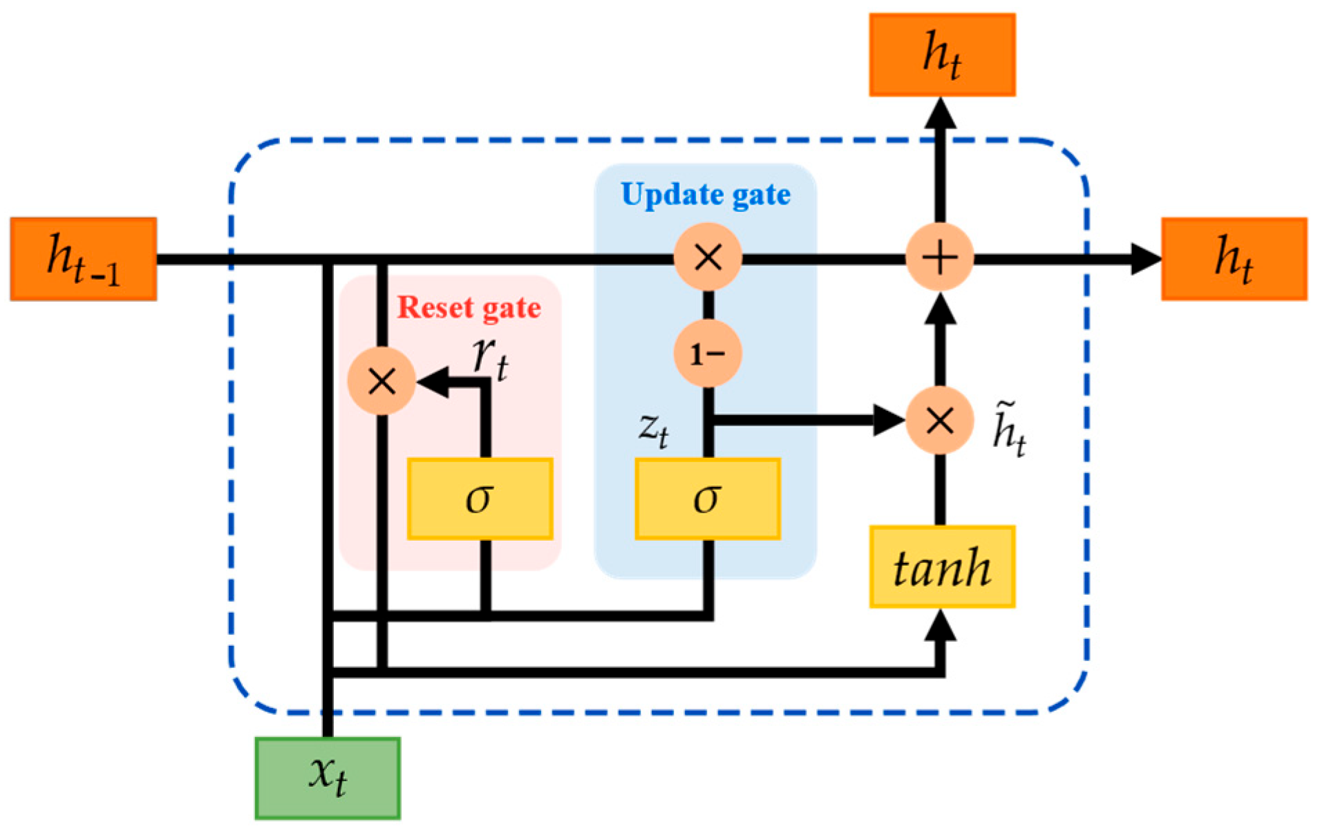
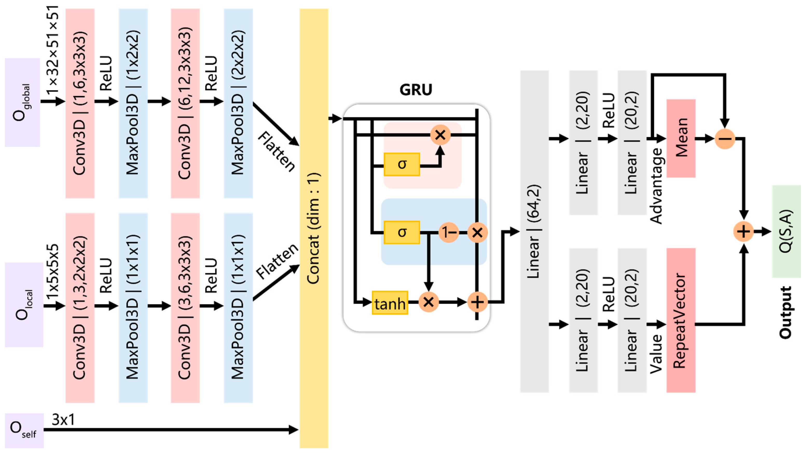
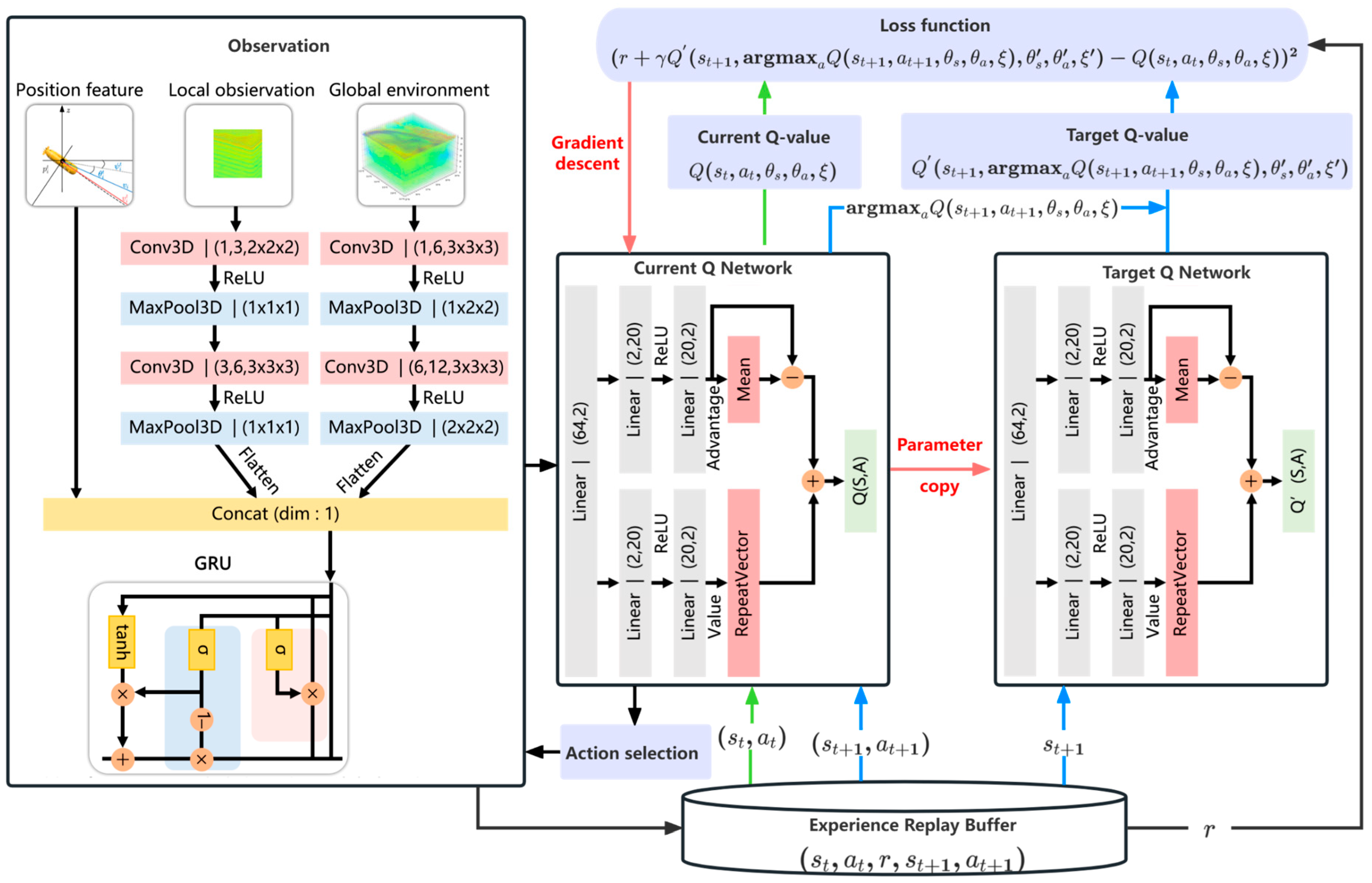
• To overcome the challenges of partial observability and the complex dynamic 3D marine environment encountered during real-world observations, we introduce a GRU-enhanced variant of the traditional D3QN algorithm, termed GE-D3QN. This enhancement accelerates the convergence of average rewards and enables state-space prediction, allowing multiple AUVs to enhance observation efficiency while effectively leveraging ocean currents to reduce energy consumption and avoid unknown obstacles.
• By conducting a series of comparative experiments and performing data assimilation on the results, we validated the effectiveness of the proposed method, demonstrating its superiority over similar algorithms in key performance indicators such as safety, energy consumption, and observation efficiency.
• To evaluate the impact of different numbers of AUV platforms on observation performance, experiments were conducted with three, five, and seven AUVs performing observation tasks simultaneously in three distinct marine environmental scenarios. A centralized training and decentralized execution approach was used, with the AUVs employing a fully cooperative observation strategy. The results indicated that while the quality of data assimilation improved with the number of AUVs, diminishing returns were observed as the number of platforms increased.

The notations used in this paper are listed in

Table A1. List of key notations.

Name	Description
$\vartheta$	Pitch angle of the AUV
$\psi$	Yaw angle of the AUV
$\varphi$	Roll angle of the AUV
$\mathit{v}$	Velocity of the AUV
$p_i^t$	Position of $i$-th AUV at time step t
${\mathit{v}}_c$	Velocity of the ocean currents
$\Delta \delta$	The angle between the AUV’s heading and the ocean current velocity
$\theta$	Parameters of current network
${\theta }^{\prime }$	Parameters of target network
${\theta }_s,{\theta }_a$	Parameters for state-value and action-value branches in current network
${\theta }_s^{\prime },{\theta }_a^{\prime }$	Parameters for state-value and action-value branches in target network
$f_c$	Current network update frequency
$f_t$	Target network update frequency
$c$	Global counter for exploration decay
$\epsilon$	Random action selection probability
$\alpha$	Learning rate
$\gamma$	Discount factor
${\epsilon }_{initial}$	Initial exploration
${\epsilon }_{decay}$	Exploration decay factor
${\epsilon }_{final}$	Final exploration
$m$	Minibatch size
$reuse\_count$	Batch reuse count
$\mathcal{D}$	Replay buffer
$\mathcal{N}$	Replay buffer capacity
$\mathcal{T}$	Total episodes

, and the subsequent sections are organized as follows: Section 2 introduces the mathematical model for multi-AUV adaptive observation, the modeling of the observational background fields, and the relevant background knowledge of DRL. Section 3 then provides a detailed explanation of the implementation of the proposed method. In Section 4, we conduct a series of simulation experiments and analyze the results. Finally, Section 5 summarizes the main contributions of this work and explores potential directions for future research.

2. Preliminaries and Problem Formulation

2.1. Problem Description

This study selects the sea area between 112° E–117° E and 15° N–20° N, extending from the surface to the seabed, as the target observation field. The temperature distribution within this region serves as the sampling data. Given the vast three-dimensional nature of the oceanic environment, areas with significant temperature variations hold greater observational value [10]. To maximize the effectiveness of AUV data collection, this study prioritizes sampling based on temperature gradients.

This section will explain the adaptive observation framework and the verification process of observation results, as well as the statement of multi-AUV adaptive ocean observation path planning.

2.1.1. Adaptive Observation Framework

Accurate information on marine environmental elements is crucial for refined ocean research. Due to the dynamic nature of the marine environment, combining numerical modeling with direct observation via AUV platforms is a key approach to obtaining reliable and effective ocean data. Data assimilation utilizes the consistency of temporal evolution and physical properties to integrate ocean observations with numerical modeling, preserving the strengths of both and enhancing forecasting system performance.

The planning and design of an adaptive observation strategy for AUVs, leveraging assimilation techniques and ocean model prediction systems, is illustrated in Figure 1. The process begins with the Princeton Ocean Model (POM), which generates daily ocean temperature simulations for the target sea area. Specifically, a five-day simulated sea surface temperature dataset serves as the prior background field for AUV operations in this study. Subsequently, the D3QN algorithm is employed to optimize the AUVs’ observation paths, ensuring efficient acquisition of ocean temperature data. The collected data are then assimilated using a coupled method based on the particle filter system described in [25], refining marine environment analysis and forecasting. This assimilation process enhances the predictive accuracy of the forecasting system, which then produces updated analysis and forecast data. These updates, in turn, guide the dynamic adjustment of the AUVs’ observation paths. This iterative cycle of data collection, assimilation, and path optimization enables continuous adaptation, ensuring that the AUVs’ observation strategy remains responsive to evolving ocean conditions.

2.1.2. Multi-AUV Adaptive Observation Path Planning

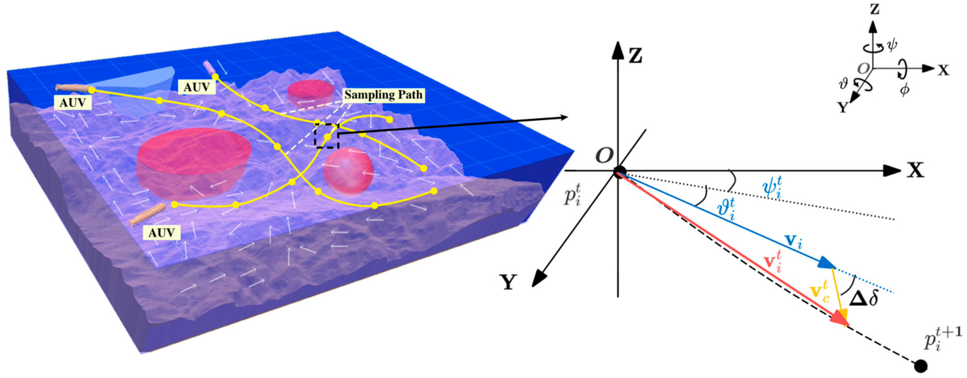
The objective of the multi-AUV adaptive marine observation strategy is to find the optimal observation path for the AUVs, maximizing the collection of ocean temperature gradient data in a 3D dynamic ocean environment affected by ocean currents, while considering the constraints of collision avoidance between AUVs and obstacle avoidance.

First, we introduce the multi-AUV systems model. Assume that the system consists of $n$ homogeneous AUVs, each equipped with sensors to gather environmental data. As illustrated in Figure 2, an AUV’s state in the Cartesian coordinate system is defined as follows:

$$\begin{array}{l}\eta =[x,y,z,\varphi ,\vartheta ,\psi {]}^T\\ v=[v_x,v_y,v_z{]}^T\end{array}$$

(1)

Here, $\eta$ denotes the AUV’s position state vector, encompassing its 3-D coordinates $p={\left[x,y,z\right]}^{\mathrm{T}}$ along with the following Euler angles: roll angle $\varphi$, pitch angle $\vartheta$, and yaw angle $\psi$. The velocity vector $v={\left[v_x,v_y,v_z\right]}^{\mathrm{T}}$ includes the velocity components along the surge (longitudinal), sway (lateral), and heave (vertical) directions. Taking into account the effects of ocean currents $v_c={\left[v_{cx},v_{cy},v_{cz}\right]}^{\mathrm{T}}$ while disregarding lateral motion and roll dynamics, the AUV’s kinematic model can be simplified as follows:

$$\left\{\begin{array}{l}\dot{x}=\left|v\right|\cos \vartheta \cos \psi +v_{cx}\hfill \\ \dot{y}=\left|v\right|\cos \vartheta \sin \psi +v_{cy}\hfill \\ \dot{z}=\left|v\right|\sin \vartheta +v_{cz}\hfill \end{array}\right.$$

(2)

Then, the Euler angles can be calculated as follows:

$$\left\{\begin{array}{l}\psi =\arctan \left({\displaystyle \frac{v_y}{v_x}}\right)\\ \vartheta =\arctan \left({\displaystyle \frac{v_z}{\sqrt{v_x^2+v_y^2}}}\right)\end{array}\right.$$

(3)

Thus, the state of the AUV can be effectively described solely by its position and translational velocity. Additionally, to mitigate the high energy costs associated with frequent acceleration and deceleration, we assume that its speed remains constant.

The schematic diagram of adaptive observation path planning for multi-AUVs is shown in Figure 2. In a 3D dynamic marine environment with obstacles $\mathbb{O}$, a team of $n$-AUVs are deployed, each traveling at a constant speed $v$ from the initial position $p_i^{t=1}=\left(x_i^{t=1},y_i^{t=1},z_i^{t=1}\right)$. Each AUV samples regions with higher temperature gradients $\Delta T$ within its observation range $d_i$, while ensuring safe navigation and fully utilizing ocean currents to reduce energy consumption. The objective is to find a path ${\mathcal{P}}_i=\{p_i^1,p_i^2,\dots ,p_i^w\}$ for each AUV that maximizes the temperature gradient at the sampling points by the end of the mission. Here, $i\in \{1,2,\dots ,n\}$, $w$ denotes the total number of sampling points along the observation path, and $p_i^w$ denotes the endpoint of the $i$-th AUV. The path from $p_i^t=\left(x_i^t,y_i^t,z_i^t\right)$ to $p_i^{t+1}=\left(x_i^{t+1},y_i^{t+1},z_i^{t+1}\right)$ for the $i$-th AUV can be expressed as follows:

$$\left\{\begin{array}{l}{x}_i^{t+1}=x_i^t+\left(v_i\cos {\vartheta }_i^t\cos {\psi }_i^t+v_{cx}^t\right)\Delta t\\ y_t^{t+1}=y_i^t+\left(v_i\cos {\vartheta }_i^t\sin {\psi }_i^t+v_{cy}^t\right)\Delta t\\ z_i^{t+1}=z_i^t+\left(v_i\sin {\vartheta }_i^t+v_{cz}^t\right)\Delta t\end{array}\right.$$

(4)

In Equation (4), ${\vartheta }_i^t$ and ${\psi }_i^t$ represent the pitch and yaw angles of the $i$-th AUV platform at the $t$-th sampling point, where $\Delta t$ is the time step. Given the assumed AUV speed and fixed observation interval, controlling ${\vartheta }_i^t$ and ${\psi }_i^t$ enables the motion control of the AUV, thereby facilitating the planning of the observation path.

In summary, the multi-AUV adaptive ocean observation path planning is formalized as the following maximization problem:

$$\begin{array}{l}{\mathcal{P}}^{\ast }=\underset{\mathcal{P}}{max}{\displaystyle \sum _{i=1}^{i=n}{\displaystyle \sum _{t=1}^{t=w}f\left(p_i^t\right)}}=\underset{\mathcal{P}}{max}{\displaystyle \sum _{i=1}^{i=n}{\displaystyle \sum _{t=1}^{t=w}\Delta T_i^t}}\\ s.t. \left\{\begin{array}{l}{\vartheta }_{\min }\le {\theta }_t^i\le {\vartheta }_{\max }\\ {\psi }_{\min }\le {\psi }_t^i\le {\psi }_{\max }\\ d=d\left(t_i\right)\\ p_i^t\notin \mathbb{O},\hspace{1em}\forall i\in \{1,2,\dots ,n\},t\in \{1,2,\dots ,w\} \end{array}\right.\end{array}$$

(5)

where $d$ represents the AUV’s endurance constraint; ${\vartheta }_{\min }$ and ${\psi }_{\min }$ denote the minimum pitch and yaw angles, respectively; and ${\vartheta }_{\max }$ and ${\psi }_{\max }$ indicate the corresponding maximum limits.

2.2. Modeling and Processing of Observational Background Fields

AUVs select areas with significant temperature gradients for observation and sampling, while avoiding obstacles such as islands, the seabed, and other hazards within the target sea area to ensure safe navigation. Additionally, the platform optimally leverages ocean current data to enhance temperature sampling efficiency. As a result, AUVs primarily focus on factors such as temperature gradients, underwater topography, obstacles, and ocean current information in the observation area. This study utilizes three-dimensional ocean temperature forecast data generated by the POM-based marine environment analysis and forecasting system, along with dynamic ocean current fields as prior background information, with temperature data serving as the primary observation target.

2.2.1. 3D Ocean Environment Forecasting and Data Processing

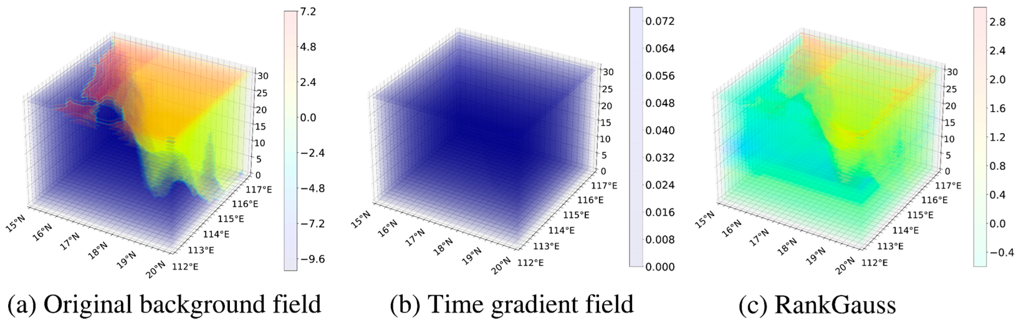
The POM, renowned for its high resolution, straightforward principles, and three-dimensional spatial characteristics, provides precise simulations of ocean conditions in estuaries and coastal regions. As one of the most widely used ocean models [26], this study uses the POM to forecast the marine environment in the observation area over the next five days. The dataset features a horizontal resolution of 1/6°, 32 vertical layers, and a temporal resolution of 6 h. The observation area extends from 112° E to 117° E and 15° N to 20° N. The spatial distribution of the forecasted sea surface temperature at a given time is illustrated in Figure 3a. To distinguish land from ocean temperature data, land areas are assigned a value of −10.

According to the literature [27], RankGauss preprocessing is particularly effective for training agents using 3D sea surface temperature data. Consequently, we apply the RankGauss method to process the observed marine area data. Using the POM, we forecasted 11 sets of data for the next 6 days. The AUV collects data every 6 h, resulting in 21 observations over the 6-day period. First, the 11 original data sets are interpolated to create 21 new sets. Next, these 21 sets undergo RankGauss preprocessing to generate the global ocean background field. Finally, the time gradient is computed from these 21 sets, yielding 20 gradient sets, which are also preprocessed using RankGauss. Figure 3 illustrates the complete data processing workflow, including the original data, the time gradient data, and the RankGauss-processed outputs.

2.2.2. Ocean Currents Modeling

AUVs routinely operate in complex and dynamic marine environments, where ocean currents have a significant impact, particularly on their kinematic parameters and trajectories. In terms of AUV planning, ocean currents inevitably affect the AUV’s trajectory during operation [23]. In a real 3D marine environment, their effects cannot be ignored, especially regarding observation time and energy consumption. When the influence of ocean currents exceeds the adjustment range of the AUV platform, the platform cannot control effectively, significantly increasing energy consumption.

Ocean currents vary with depth, and to reach sampling points within the designated observation time, AUVs must strategically navigate by leveraging favorable currents and avoiding unfavorable ones through depth adjustments, such as diving or surfacing [28]. Current data can be obtained through various methods, such as ocean hydrographic observatories, satellite remote sensing technology, and current meters. Some of these datasets are widely recognized for their applications in marine research. The dataset used in this study is the China Ocean ReAnalysis version 2 (CORAv2.0) [29] reanalysis dataset from the National Ocean Science Data Center (NOSDC). It provides daily average data for 2021 with a spatial resolution of 1/10°. To match the 1/6° resolution of the POM model, the CORAv2.0 data are downsampled from their original 1/10° resolution. The temporal resolution is also improved from 24-h to 6-h updates.

As shown in Figure 4, the observed background field consists of 3D regional ocean temperature gradient data from the marine environment numerical prediction system that incorporates ocean currents.

2.3. Deep Reinforcement Learning

The Markov decision process (MDP) serves as a fundamental framework for modeling sequential decision-making problems and forms the theoretical basis of reinforcement learning. In an MDP, state transitions are determined solely by the current state. However, real-world environments rarely adhere to the ideal assumptions of MDPs. In contrast, the POMDP provides a rigorous mathematical framework for sequential decision-making under uncertainty [30]. POMDPs do not assume that the agent has access to the true underlying state, which is a practical assumption for real-world systems, as AUVs typically have limited information about the underlying target phenomena and even their own state in practice. Consequently, the multi-AUV observation problem can be framed as a POMDP.

A POMDP is commonly represented by the tuple $〈\mathcal{S},\mathcal{A},\mathcal{O},T,{\rm Z},R,\gamma 〉$. In this formulation, $\mathcal{S}$ represents the state space, $\mathcal{A}$ the action space, and $\mathcal{O}$ the observation space. The transition function $T$ determines the probability of transitioning to state $s^{\prime }$ when action $a$ is taken in state $s$, expressed as $T(s,a,s^{\prime })=P(s^{\prime }|s,a)$. Likewise, the observation function ${\rm Z}(s^{\prime },a,o)=P(o\mid s^{\prime },a)$ represents the probability of receiving observation $o$ once the agent executes action $a$ and transitions to state $s^{\prime }$. The reward function $R(s,a)$ determines the expected immediate reward that an agent receives after performing action $a$ in state $s$. In infinite-horizon settings, a discount factor $\gamma \in \left[\begin{array}{c}0,1\end{array}\right]$ is employed to guarantee that the overall expected reward $\mathbb{E}\left[{\displaystyle \sum _{t=0}^{\infty }}{\gamma }^{t}R(s_t,a_t)\right]$ remains finite. Ultimately, the goal is to derive an optimal policy that maximizes the expected cumulative reward over the trajectory.

In practical applications, optimally solving POMDPs is computationally challenging. However, various DRL algorithms can provide feasible solutions. DRL enables agents to interact with the environment and learn through feedback in the form of rewards or penalties. DRL provides a powerful framework for adaptive observation strategy optimization. By learning to optimize actions to maximize ocean environment information gain, DRL-based systems can adaptively and efficiently explore unknown environments.

DRL integrates reinforcement learning with the powerful function approximation capabilities of deep neural networks. In DRL, deep neural networks serve as models to estimate or optimize policies and value functions in POMDP problems. DQN is one of the most renowned DRL methods, employing deep neural networks to approximate the value function. It utilizes Q-learning to generate Q-network samples, effectively aligning the estimated Q-value with the target Q-value. To achieve this, a loss function is formulated, and the network parameters are refined using gradient descent via backpropagation. The target Q-value is computed as follows:

$$Q(s,a;\theta )=r_{t+1}+\gamma \underset{a^{\prime }}{\max }Q(s^{\prime },a^{\prime };{\theta }^{\prime })$$

(6)

where $\theta$ and ${\theta }^{\prime }$ denote the weighting parameters of the neural network and the target network, respectively. Additionally, ${\max }_{a^{\prime }}Q$ represents the action with the highest Q-value. In this work, the agent aims to maximize cumulative rewards from the environment using the Q-value and execute the optimal policy through ${\max }_{a^{\prime }}Q$. The DQN loss function is expressed as follows:

$$L(\theta )=\mathbb{E}\left[{(r_{t+1}+\gamma \underset{a^{\prime }}{\max }Q(s^{\prime },a^{\prime };{\theta }^{\prime })-Q(s,a;\theta ))}^2\right]$$

(7)

Here, $\mathbb{E}\left[\cdot \right]$ denotes the expected value, calculated as an average over all possible state transitions in the loss function.

DQN calculates the target Q-value by selecting the maximum Q-value at each step using the $\epsilon$-greedy algorithm, which can lead to overestimation of the value function. To address this issue, algorithms such as DDQN [19] and D3QN [22] have been proposed. The learning strategy of D3QN is more efficient, and its performance has been proven in many applications. In this paper, we use D3QN to implement adaptive observation strategy planning in multi-AUV scenarios.

3. Methodology

3.1. POMDP for Multi-AUV Adaptive Observation

In this section, we present the POMDP framework designed for the multi-AUV adaptive observation path planning problem. The framework clearly defines the state and observation spaces to capture the uncertainties of the marine environment, specifies the set of available actions, and formulates the reward functions that guide the decision-making process.

3.1.1. State and Observation Space

In this study, to achieve the sampling objective in the regional marine environment, the state space is composed of three components: $O_{global}$, representing the global background field; $O_{local}$, capturing observations of the surrounding environment; and $O_{self}$, indicating the AUV’s current position. Thus, the state is defined as $O=[O_{global},O_{local},O_{self}]$.

$O_{global}$ encompasses information on the global ocean environment field, as well as the temporal gradient field of the ocean environment. The observation state of the surrounding environment $O_{local}$ includes local ocean environment field data around the AUV, the temporal gradient of the local ocean environment, and obstacle information. The state $O_{self}={[x,y,z]}^T$ represents the AUV’s position in the inertial coordinate system.

3.1.2. Action Space

As demonstrated in Section 2.1.2, AUV motion control can be effectively achieved by adjusting the pitch and yaw angles. Given the discrete nature of executable actions generated by neural network outputs, excessive action dimensionality would prolong training convergence. Consequently, the action space $\mathcal{A}$ consists of the AUV’s pitch angle $\vartheta$ and yaw angle $\psi$. During the AUV’s observation process, we assume that both the heading and pitch angles are within ±30°. The action dimension is set to 8, meaning that both the heading and pitch angles are divided into 8 equal segments, i.e.,

$$\vartheta =\left[-30°,-22.5°,-15°,-7.5°,0°,7.5°,15°,22.5°,30°\right], \psi =\left[-30°,-22.5°,-15°,-7.5°,0°,7.5°,15°,22.5°,30°\right].$$

The action space is designed this way because uncertainty in 3D space is too complex. Therefore, the simpler the action space, the more effective it is for AUV control.

3.1.3. Reward Functions

This study adopts a multi-platform collaborative approach to ocean data sampling missions, with the aim of achieving more efficient observations in a 3D, time-varying marine environment. We assume that each AUV is homogeneous and has the same mission objective, which encourages a fully cooperative relationship between AUV platforms. Such problems can be solved by maximizing the joint reward. Therefore, the reward function for multi-AUV cooperative observation can be designed as the sum of the rewards of all AUV platforms.

$$R_t={\displaystyle \sum _{i=1}^n{r}_t^i}$$

(8)

In Equation (8), $r_t$ represents the reward value obtained by an AUV platform during a round of path planning.

The reward functions design aims to guide the AUVs to sample data with significant temperature gradients within the specific ocean area, while satisfying constraints such as collision avoidance, obstacle avoidance, and energy efficiency. Therefore, the individual reward architecture is partitioned into five components: sampling reward $r_{grad}$, collaborative reward $r_{collab}$, current utilization reward $r_{cur}$, collision reward $r_{obst}$, and range reward $r_{range}$. Furthermore, to encourage AUVs to move along the direction of ocean currents and thereby collect ocean data more efficiently with lower energy consumption, we set the current utilization reward as a weighting coefficient of the sampling reward. Thus, the individual reward function can be expressed as follows:

$$r_t^i=\left(1+r_{cur}^i\right)r_{grad}^i+r_{collab}^i+r_{obst}^i+r_{range}^i$$

(9)

(1)

Sampling reward

To obtain ocean temperature data with a large temporal gradient, a reward function $r_{grad}^i$ is designed in which the reward value is positively correlated with the ocean temperature gradient. A penalty is applied if the gradient is too small.

$$r_{grad}^i=\left\{\begin{array}{ll}\hfill 10,\hfill & \hfill grad\left(\Delta T\right)\ge 3\\ \hfill 8,\hfill & \hfill 2\le grad\left(\Delta T\right)<3\\ \hfill 6,\hfill & \hfill 1\le grad\left(\Delta T\right)<2\\ \hfill 4,\hfill & \hfill 0\le grad\left(\Delta T\right)<1\\ \hfill 2,\hfill & \hfill -1\le grad\left(\Delta T\right)<0\\ \hfill 0,\hfill & \hfill -2\le grad\left(\Delta T\right)<-1\\ \hfill -1,\hfill & \hfill -3\le grad\left(\Delta T\right)<-2\\ \hfill -2,\hfill & \hfill otherwise\end{array}\right.$$

(10)

(2)

Collaborative reward

In multi-AUV cooperative observation, sampling redundancy at time $t$ must be considered. Rewards for nearby samples are treated as a single unique sample, requiring adjustment based on redundancy. The closer the AUVs are, the higher the redundancy. The collaborative reward aims to encourage distributed regional sampling, maximizing coverage while avoiding excessive clustering, redundant sampling, and potential collisions.

However, maintaining a minimum distance between AUVs is essential for effective communication and sampling data sharing. The collaborative reward formula should consider AUV dispersion and communication range, encouraging a balance between maximizing coverage and enabling efficient information exchange.

Therefore, the expression for the collaborative reward $r_{collab}^i$ is as follows:

$$\begin{array}{l}{r}_{collab}^i=\left\{\begin{array}{l}-10,\hspace{1em}\hspace{1em}{d}_{ij}<d_{\min }\\ {\displaystyle \frac{k}{n}}{\displaystyle \sum _{i\ne j}{d}_{ij}}, \mathit{otherwise}\end{array}\right.\\ with\hspace{1em}i=1,\dots ,n; j=1,\dots ,n; i\ne j\end{array}$$

(11)

In Equation (11), $d_{ij}$ represents the distance between the $i$-th AUV and each other, while $d_{\min }$ is the safe distance. The collaborative reward will be proportional to the average distance between agent $i$ and the others. If $d_{ij}<d_{\min }$, the AUVs are too close together, which may lead to a collision, resulting in a negative reward.

(3)

Ocean currents utilization reward

During AUV sampling missions, ocean currents play a pivotal role as they significantly influence both the velocity and energy consumption of the AUV. To harness the beneficial effects of ocean currents in reducing travel time and energy usage, we propose a specialized reward function that factors in these currents.

$$r_{cur}^i=\cos \left(\Delta \delta \right)$$

(12)

This function incorporates the angle $\Delta \delta$ between the AUV’s heading direction and the direction of the ocean current velocity. A smaller $\Delta \delta$ yields a higher reward, thereby encouraging trajectories that take advantage of favorable current conditions.

(4)

Collision reward

The collision reward here mainly considers collisions between the AUV platform and obstacles in the marine environment. Collisions among multiple AUV platforms are accounted for in the collaboration reward and are not considered here. When the AUV platform collides with an obstacle, a substantial penalty is imposed. The collision reward is formulated as follows:

$$r_{obst}^i=\left\{\begin{array}{l}-10,\mathit{collision}\\ \hspace{1em}0,\mathit{otherwise}\end{array}\right.$$

(13)

(5)

Range reward

A constraint is imposed on the position of the AUV platform, and a penalty is applied if the sampling path exceeds the specified range. The range reward can be expressed as follows:

$$r_{range}^i=\left\{\begin{array}{l}-10,\mathit{out} \mathit{of} \mathit{range}\\ \hspace{1em}0,\mathit{otherwise}\end{array}\right.$$

(14)

3.2. Adaptive Observation Method Based on Deep Reinforcement Learning

3.2.1. D3QN Algorithm

D3QN combines two methods: the Dueling Architecture and Double DQN, combining their strengths. The Dueling Architecture separates the estimation of state value and action advantage functions, enabling a more precise and independent evaluation of each state’s value and the relative importance of each action. This enhances the agent’s ability to determine the most optimal action. Double DQN mitigates the issue of Q-value overestimation by curbing the agent’s tendency to overvalue specific actions, leading to more stable and accurate learning outcomes.

The Dueling Architecture separates the Q-value being learned by an agent into two components. The first component is the state value function $V(s)$, which quantifies the inherent value of a given state. The second component is the action value function $A(s,a)$, which reflects the relative value of performing a particular action in that state. These two components are combined through summation to produce the final Q-value, as shown in Equation (15).

$$Q(s,a;{\theta }_s,{\theta }_a,\xi )=V(s;\theta ,\xi )+\left(A\left(s,a;{\theta }_s,{\theta }_a,\xi \right)-avg\left(A\left(s,a^{\prime };{\theta }_s,{\theta }_a,\xi \right)\right)\right)$$

(15)

in which

$$avg\left(A\left(s,a^{\prime };{\theta }_s,{\theta }_a,\xi \right)\right)={\displaystyle \frac{1}{\left|\mathcal{A}\right|}}\sum _{a^{\prime }\in \mathcal{A}}A(s,a^{\prime };{\theta }_s,{\theta }_a,\xi )$$

(16)

where $s$, $a$ represent each state–action pair. The parameters ${\theta }_s$ and ${\theta }_a$ correspond to the state value function and the action value function, respectively, while $\xi$ is the common parameter shared by both. Additionally, $\left|\mathcal{A}\right|$ represents all possible actions.

By combining the advantages of Double DQN, D3QN utilizes two Q-networks to avoid overestimation of the Q-value. Specifically, the current Q-network selects an action, while the target Q-network estimates the Q-values of the selected action. To update the network parameters, D3QN selects actions through the current network:

$$a^{\prime }=\arg \underset{a}{\max }Q\left(s^{\prime },a;{\theta }_s,{\theta }_a,\xi \right)$$

(17)

The target network computes the Q-value corresponding to the state–action pair $Q^{\prime }(s^{\prime },a^{\prime };{\theta }_s^{\prime },{\theta }_a^{\prime },{\xi }^{\prime })$. By separating the processes of action selection and value evaluation, this update mechanism effectively addresses the issue of overestimation. The loss function is defined as follows:

$$\begin{array}{ll}\mathit{Loss}& =\mathbb{E}\left[{\left(r+\gamma Q^{\prime }\left(s^{\prime },a^{\prime };{{\theta }^{\prime }}_s,{{\theta }^{\prime }}_a,{\xi }^{\prime }\right)-Q\left(s,a;{\theta }_s,{\theta }_a,\xi \right)\right)}^2\right]\\ & =\mathbb{E}\left[{\left(r+\gamma Q^{\prime }\left(s^{\prime },\arg \underset{a^{\prime }}{\max }Q(s^{\prime },a^{\prime };{\theta }_s,{\theta }_a,\xi );{{\theta }^{\prime }}_s,{{\theta }^{\prime }}_a,{\xi }^{\prime }\right)-Q\left(s,a;{\theta }_s,{\theta }_a,\xi \right)\right)}^2\right]\end{array}$$

(18)

3.2.2. GE-D3QN for Multi-AUV Adaptive Observation Path Planning

The D3QN architecture leverages the strengths of Dueling DQN and Double DQN, utilizing a dual-branch framework for Q-value estimation and incorporating distributed learning mechanisms. While demonstrating superior capability in processing high-dimensional state representations through its network structure, particularly in precisely addressing multi-factor environmental complexity, the approach exhibits inherent limitations in limited partial observability and complex agent–environment interactions. These deficiencies compromise system autonomy and observation effectiveness during adaptive observation path planning for multi-AUV systems in complex ocean environments. To overcome these challenges, we propose a novel GE-D3QN architecture integrating GRU modules, forming a comprehensive optimization framework for multi-AUV cooperative observation path planning in dynamic marine environments.

In multi-AUV adaptive observation within dynamic ocean environments, the observation process of mobile ocean platforms essentially follows a POMDP. Traditional D3QN algorithms struggle to adapt effectively to such environments. To address this issue, LSTM networks [31] are commonly used; however, in this study, we explore the use of GRU networks. Therefore, we enhance the neural network architecture of the D3QN algorithm by integrating a GRU network, endowing the algorithm with memory capability. This improvement strengthens the algorithm’s ability to correlate current inputs with previous observations, enabling it to leverage both historical and current states for more informed decision-making in ocean data sampling and processing. Additionally, the enhanced algorithm improves exploration efficiency through its refined neural network structure.

The GRU [32] is a variant of the LSTM network. While LSTM effectively addresses issues such as long-term dependencies, vanishing gradients, and exploding gradients, its structure is relatively complex, leading to high computational costs. GRU optimizes the recurrent unit structure by reducing LSTM’s three gating mechanisms to two: the reset gate and the update gate. This enhancement improves prediction efficiency while maintaining accuracy, reducing training time, and enhancing the model’s real-time performance. Figure 5 provides an illustration of the GRU architecture.

The operational mechanism can be described as follows: First, the previous hidden state $h_{t-1}$ and current input $x_t$ are concatenated into a joint vector $\left[h_{t-1},x_t\right]$, which is subsequently processed through the reset gate. This gate utilizes a sigmoid activation function $\sigma$ to generate a reset signal $r_t$, selectively filtering past state information and producing an updated state $r_t·h_{t-1}$.

$$r_t=\sigma \left(W_r\cdot \left[h_{t-1},x_t\right]\right)$$

(19)

Next, the update gate processes $\left[h_{t-1},x_t\right]$ through a sigmoid activation function, generating $z_t$, which controls the retention of past information.

$$z_t=\sigma \left(W_z\cdot \left[h_{t-1},x_t\right]\right)$$

(20)

After that, the modified previous state $r_t·h_{t-1}$ is combined with the current input $x_t$ to form a new vector $\left[r_t\cdot h_{t-1},x_t\right]$, which undergoes transformation through a tanh activation function, producing the candidate state ${\tilde{h}}_t$.

$${\tilde{h}}_t=\tanh \left(W_{\tilde{h}}\odot \left[r_t\cdot h_{t-1},x_t\right]\right)$$

(21)

Finally, a selective update mechanism integrates essential information from both the past state $h_{t-1}$ and the candidate state ${\tilde{h}}_t$, determining the final output of the current layer, as defined in Equation (22).

$$h_t=\left(1-z_t\right)\odot h_{t-1}+z_t\odot {\tilde{h}}_t$$

(22)

where $\odot$ is the Hadamard product, and $W_r$, $W_z$, and $W_{\tilde{h}}$ represent the corresponding weight matrices.

The structure of the GE-D3QN network is shown in Figure 6. First, a convolutional network extracts both global and local environmental features, followed by max pooling for dimensionality reduction. These extracted features, along with the current position information, are then fed into a GRU module with memory capability. This module, comprising 256 neurons, endows the algorithm with long-term memory, enabling the AUV to integrate both historical and current states for more informed decision-making. The GRU module’s output is subsequently processed through a fully connected layer, which connects to both the value and advantage functions. The value function assesses the current state and predicts the expected reward, while the advantage function, sharing the same dimensionality as the action space, determines the relative benefit of each action compared to the average. As a result, the advantage function provides an advantage value for each possible action, refining the decision-making process.

In designing our network architecture, we evaluated the influence of key parameters—including network depth, convolution kernel size, pooling layer configuration, GRU hidden neuron count, and the choice of activation function—on overall performance. Our initial settings were guided by prior research [33,34,35]. As depicted in Figure 6, the global environmental input has dimensions of 1 × 32 × 51 × 51. To efficiently capture spatiotemporal features while keeping computational demands in check, we chose a 3 × 3 × 3 convolution kernel; for dimensionality reduction, we used pooling kernels of either 1 × 2 × 2 or 2 × 2 × 2 to retain as much information as possible. In contrast, the local observation state, with a smaller input size of 1 × 5 × 5 × 5, utilizes a 2 × 2 × 2 convolution kernel and a 1 × 1 × 1 pooling kernel (i.e., no downsampling) to preserve critical features. We adopted the ReLU activation function to enhance the model’s capacity for processing highly nonlinear data. Regarding the GRU layer, although a neuron count between 128 and 512 is common, we selected 256 neurons to balance the need for sufficient capacity to capture complex temporal dependencies against the risk of overfitting and excessive computational cost. Finally, the overall network depth and the number of nodes in the fully connected layers were determined based on the dimensions of the state and action spaces and fine-tuned through experiments to achieve an optimal trade-off between accuracy and efficiency.

In this study, our problem is fully cooperative, and since the agents are homogeneous in terms of actions and observation capabilities, we adopt a centralized training strategy to fully utilize global information for optimizing the observation path planning strategy. Figure 7 shows a schematic diagram of the GE-D3QN algorithm.

First, GE-D3QN integrates both global and local marine environmental information, along with position data, into the state input of the neural network, enabling multi-AUV to intelligently utilize ocean currents for observation path planning, thereby enhancing flexibility and adaptability.

In DRL, balancing exploration and exploitation is crucial. Agents must navigate between leveraging past experiences to make informed decisions and exploring new environments to uncover better solutions. Excessive reliance on prior knowledge can result in convergence to suboptimal policies, while too much exploration may extend training time and reduce efficiency. To mitigate this challenge, we implement a strategy that progressively decreases the probability of selecting random actions, ensuring a smooth transition from exploration to exploitation.

$$\epsilon ={\epsilon }_{final}+({\epsilon }_{initial}-{\epsilon }_{final})e^{{\displaystyle \frac{-c}{{\epsilon }_{decay}}}}$$

(23)

This ensures that as the global counter $c$ increases, the exploration probability gradually decreases. Here, ${\epsilon }_{initial}$, ${\epsilon }_{final}$, and ${\epsilon }_{decay}$ represent the initial exploration rate, final exploration rate, and exploration decay factor, respectively. The action selection mechanism is defined as follows:

$$a=\left\{\begin{array}{ll}\mathit{randomly} \mathit{chosen} a\in \mathcal{A},& \mathit{with} \mathit{probability} \epsilon \hfill \\ \underset{a}{\arg \max }{Q}_{\pi }\left(s,a;{\theta }_s,{\theta }_a\right),& \mathit{with} \mathit{probability} 1-\epsilon \hfill \end{array}\right.$$

(24)

To address the challenge of partial observability and effectively leverage ocean current information in real-time, we incorporate a GRU into the deep neural network. Structurally, GE-D3QN uses a Convolutional Neural Network (CNN) layer to extract spatial features, while the GRU module captures temporal dependencies between action sequences, thereby improving learning performance. The GE-D3QN network is then divided into two branches, separately estimating state and action values. By decoupling the state and action values and separating action selection from value prediction, the algorithm effectively mitigates the overestimation problem, resulting in more stable and reliable observation path planning. The parameter update and iterative process of the GE-D3QN algorithm are detailed in Algorithm 1.

Algorithm 1: GE-D3QN Algorithm
1:	Initialize: current network with parameters ${\theta }_s,{\theta }_a$, target network with parameters ${\theta }_s^{\prime },{\theta }_a^{\prime }$${\theta }_s^{\prime }\leftarrow {\theta }_s$ and ${\theta }_a^{\prime }\leftarrow {\theta }_a$, minibatch size m, replay buffer capacity $\mathcal{N}$, total episodes $\mathcal{T}$, Maximum time steps per episode $T_{\max }$, learning rate $\alpha$, discount factor $\gamma$
2:	Global counter c = 0
3:	for n = 1 to $\mathcal{T}$ do
4:	t = 0, done = false, reset environment and get initial state s0
5:	While not done and $t\le T_{\max }$ do
6:	Select action using Equation (24)
7:	Execute action and receive reward $r_t$ and next state $s_{t+1}$
8:	Fill replay buffer $\mathcal{D}$ with experiences $(s_t,a_t,r_t,s_{t+1})$
9:	$t=t+1$$, c=c+1$
10:	if n mod fc == 0 then  #Update current network
11:	Sample m group experience
12:	for   $j=1$ to $m$ do
13:	Optimal action via current network based on Equation (17)
14:	Calculate update target $y_t=r_t+\gamma Q^{\prime }\left(s_{t+1},a_{t+1};{{\theta }^{\prime }}_s,{{\theta }^{\prime }}_a,{\xi }^{\prime }\right)$
15:	end for
16:	Calculate loss function using Equation (18)
17:	Update parameters $\left({\theta }_s,{\theta }_a\right)\leftarrow \left({\theta }_s,{\theta }_a\right)+\alpha {\nabla }_{\left({\theta }_s,{\theta }_a\right)}\mathit{Loss}$
18:	end if
19:	if n mod $f_t==0$ then  #Update target network
20:	Copy from the current network ${\theta }_s^{\prime }\leftarrow {\theta }_s$$,{\theta }_a^{\prime }\leftarrow {\theta }_a$
21:	end if
22:	end while
23:	end for

4. Simulation Results and Discussions

Based on the multi-AUV adaptive observation strategy developed in the above research, we set up several simulation scenarios to validate the effectiveness of the proposed method. Additionally, to demonstrate the superiority of the GE-D3QN algorithm proposed in this study, we incorporated the widely-used RNN and LSTM networks with the D3QN algorithm, forming the RE-D3QN and LE-D3QN algorithms. Comparison experiments were then conducted using D3QN, RE-D3QN, and LE-D3QN as benchmark algorithms.

The simulation experiments in this study were conducted on a system equipped with an Intel Core™ i7-12700F CPU (Intel Corporation, Santa Clara, CA, USA) and an NVIDIA GeForce RTX 3070 graphics card (8GB GDDR6), accompanied by 16GB DDR4 system memory. The algorithm was developed using Python 3.11 and PyTorch 2.0.1.

4.1. Parameter Setting

The initial hyperparameter settings for the algorithm are based on relevant literature [23,36,37]. The learning rate $\alpha$ controls the magnitude of weight updates during backpropagation of the neural network. If $\alpha$ is too high, it can lead to large updates and unstable convergence; conversely, if it is too low, it slows convergence speed and reduces learning performance. To improve convergence, this study uses the Adam optimizer with a learning rate of $1\times 10^{-4}$. The discount factor $\gamma$, which governs the agent’s emphasis on future rewards and ranges between 0 and 1, is set to 0.9 to ensure a balanced consideration of immediate and long-term rewards. To encourage exploration and avoid local optima, the initial exploration rate is set to 1.0 and gradually decreases with a decay factor of 0.995. Over multiple training episodes, the exploration rate stabilizes at 0.05.

The exploration rate stabilizes at 0.05. The experience pool capacity is set to $1\times 10^6$. The batch size, which defines the number of samples randomly selected per iteration, balances update consistency with computational efficiency. Based on available memory, it is set to 64. Each batch is reused four times for parameter updates to maximize data efficiency, though excessive reuse may lead to overfitting.

The experimental results indicate that after 4000 training episodes, performance stabilizes. Thus, the total number of training episodes is set to 5000 for a comprehensive evaluation of different algorithms. The main algorithm parameters are summarized in

Table 1. Main hyperparameter settings for the algorithm.

Parameters	Symbol	Value
Learning rate	$\alpha$	$1\times {10}^{-4}$
Discount factor	$\gamma$	0.9
Initial exploration	${\epsilon }_{initial}$	1.0
Exploration decay factor	${\epsilon }_{decay}$	0.995
Final exploration	${\epsilon }_{final}$	$1\times {10}^{-4}$
Minibatch size	$m$	64
Batch reuse count	$reuse\_count$	4
Replay buffer capacity	$\mathcal{N}$	$1\times 10^6$
Total episodes	$\mathcal{T}$	$5\times 10^3$

.

The experimental environment is a 3D dynamic ocean background field generated by the POM model. Background data spanning six consecutive days are used, with updates every 6 h. Each training session includes 21 samples collected by the AUV platform. Each algorithm undergoes training in 50 groups, with 5000 episodes per group.

4.2. Scenario 1: Multi-AUV Observation Path Planning in Marine Environment Without Currents

This section presents a multi-AUV collaborative observation experiment in a current-free environment (i.e., the background field constructed in Section 2.2.1). Four algorithms—D3QN, RE-D3QN, LE-D3QN, and GE-D3QN—are used to perform collaborative observations in this environment. The experiment consists of five AUV platforms, each navigating at a speed of 7 km/h, whose initial positions are listed in

Table 2. Starting position settings for multi-AUVs in current-free environments.

Scenario	Platform	Starting Position
Multi-AUV observation situation without ocean current	AUV 1	[112.4° E, 15.9° N, 5th layer]
	AUV 2	[112.4° E, 16.5° N, 10th layer]
	AUV 3	[112.4° E, 17.5° N, 15th layer]
	AUV 4	[112.4° E, 18.5° N, 20th layer]
	AUV 5	[112.4° E, 19.5° N, 25th layer]

.

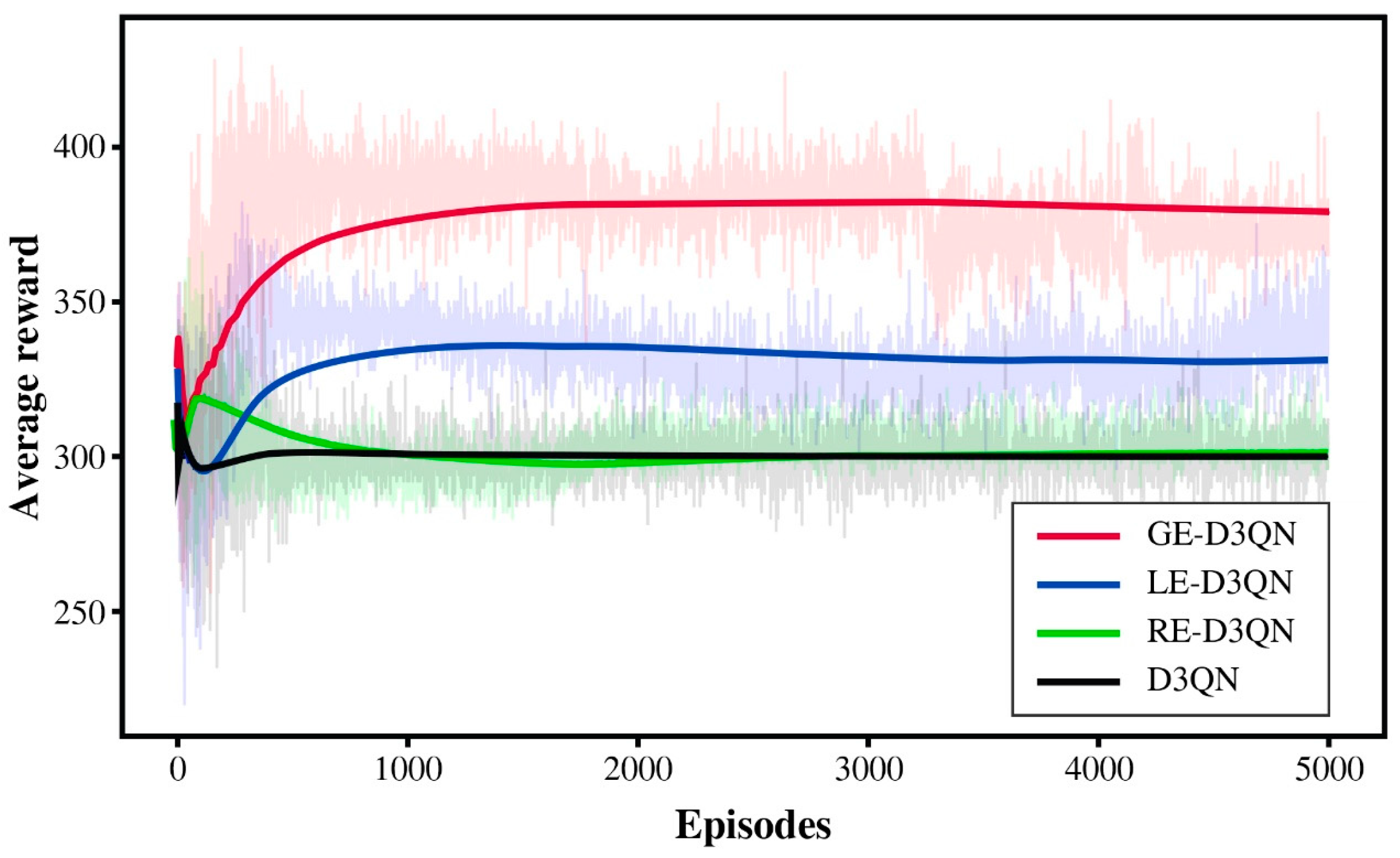
As shown in Figure 8, after the initial phase of random exploration, the reward value of the D3QN algorithm follows a slow upward trend. However, in subsequent rounds of exploration, its training performance improves at a sluggish pace and eventually falls into a local optimum.

In contrast, the RE-D3QN algorithm benefits from the memory function of the neural network, allowing it to achieve a relatively high reward value during the initial exploration phase. However, as training progresses, the model increasingly learns interference signals, leading to a decline in reward value after the initial exploration stage. Consequently, the total reward value of the five agents stabilizes around 300, with no significant fluctuations.

Meanwhile, LE-D3QN, with its integrated forget gate mechanism, gradually filters out unimportant interference information during training, thereby maintaining better learning performance. GE-D3QN, leveraging its unique gated parameter adjustment mechanism, continuously optimizes its gating parameters during exploration to adapt to environmental changes, resulting in superior training outcomes.

Analyzing the reward curves of the four algorithms, LE-D3QN and GE-D3QN demonstrate relatively stable learning trends with a continuous upward trajectory. Notably, after 3000 episodes, GE-D3QN experiences a brief decline in reward value but quickly rebounds. This suggests that the algorithm retains its exploratory capability even when trapped in a local optimum, allowing it to break through and further enhance the optimization of the observation strategy.

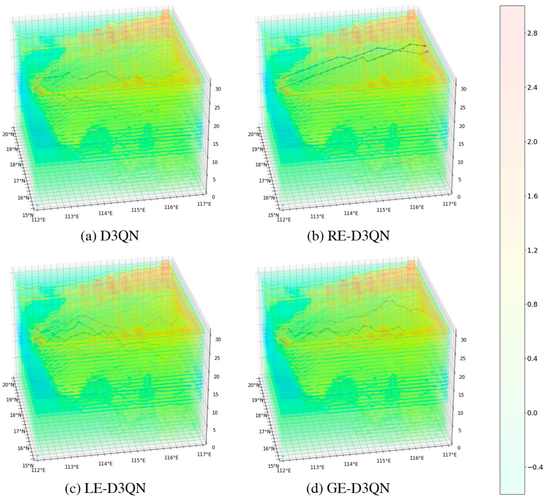
Figure 9 presents the observation paths that achieved the highest reward values after 5000 episodes for the four algorithms. The figure shows that the AUVs are capable of sampling regions with significant temperature differences. Among the five paths planned by each algorithm, the D3QN algorithm’s path appears relatively smooth, indicating insufficient exploration of the surrounding environment, which results in lower reward values. The RE-D3QN algorithm follows a straight-line exploration pattern, suggesting that it has fallen into a local optimum during discrete action selection. This occurs because a specific action previously yielded a high reward, causing the algorithm to repeatedly execute similar actions in subsequent path planning. In contrast, the paths planned by LE-D3QN and GE-D3QN are more intricate, demonstrating that these two algorithms can fully explore the surrounding environment and thus generate more optimal, high-reward paths.

A total of 50 training groups were conducted for the four algorithms—D3QN, RE-D3QN, LE-D3QN, and GE-D3QN. From these, the three best-performing datasets were selected. The observation strategies with the highest rewards were identified, and temperature data were collected from their respective sampling points. Subsequently, particle filtering was applied for data assimilation, using the Root Mean Square Error (RMSE) between forecasted and actual values as the evaluation criterion. A comparative analysis was then performed to assess the sampling performance of the four algorithms against random sampling, evaluating the impact of different observation strategies on improving the forecasting system’s performance. The RMSE calculation formula is as follows:

$$RMSE=\sqrt{{\displaystyle \frac{1}{M}}{\displaystyle \sum _{i=1}^M{\left({\overline{z}}_i-z_i^t\right)}^2}}$$

(25)

Here, $M$ represents the number of analysis steps used for the statistical computation, while ${\overline{z}}_i$ and $z_i^t$ represent the ensemble mean corresponding to the model state $z$ and the true value, respectively.

As shown in

Table 3. RMSE comparison of assimilation results for the observation paths of four algorithms in current-free environments.

GE-D3QN	LE-D3QN	RE-D3QN	D3QN	Random
0.4718 °C	0.4851 °C	0.5043 °C	0.5341 °C	0.5793 °C
0.4697 °C	0.4883 °C	0.5067 °C	0.5409 °C	0.5835 °C
0.4659 °C	0.4792 °C	0.4983 °C	0.5315 °C	0.5864 °C

, with the RMSE of random sampling serving as the baseline for the forecasting system’s performance, the average RMSE for the three selected observation strategies was calculated, enabling a comparison of performance improvements across the four algorithms. The results indicate that D3QN, RE-D3QN, LE-D3QN, and GE-D3QN improved forecasting performance by 8.158%, 13.715%, 16.956%, and 19.540%, respectively. These findings demonstrate that employing the GE-D3QN algorithm for observation strategy design significantly enhances the accuracy and effectiveness of the ocean forecasting system.

4.3. Scenario 2: Multi-AUV Observation Path Planning in Marine Environment with Ocean Currents

This section simulates the collaborative observation of multi-AUVs under the influence of ocean currents. Dynamic ocean currents (as described in Section 2.2.2) were introduced into the background field, with their direction and speed varying over time. To evaluate the observation efficiency of multi-AUVs in this environment, we conducted experiments using four algorithms: D3QN, RE-D3QN, LE-D3QN, and GE-D3QN, under ocean current perturbations. Due to the stronger currents near the sea surface, the starting positions of the AUVs were set close to the surface to better capture the ocean current variations, as detailed in

Table 4. Starting position settings for multi-AUVs in ocean current environments.

Scenario	Platform	Starting Position
Multi-AUV observation situation with ocean currents	AUV 1	[117° E, 16.0° N, 28th layer]
	AUV 2	[117° E, 16.8° N, 26th layer]
	AUV 3	[117° E, 17.5° N, 24th layer]
	AUV 4	[117° E, 18.6° N, 26th layer]
	AUV 5	[117° E, 19.5° N, 28th layer]

.

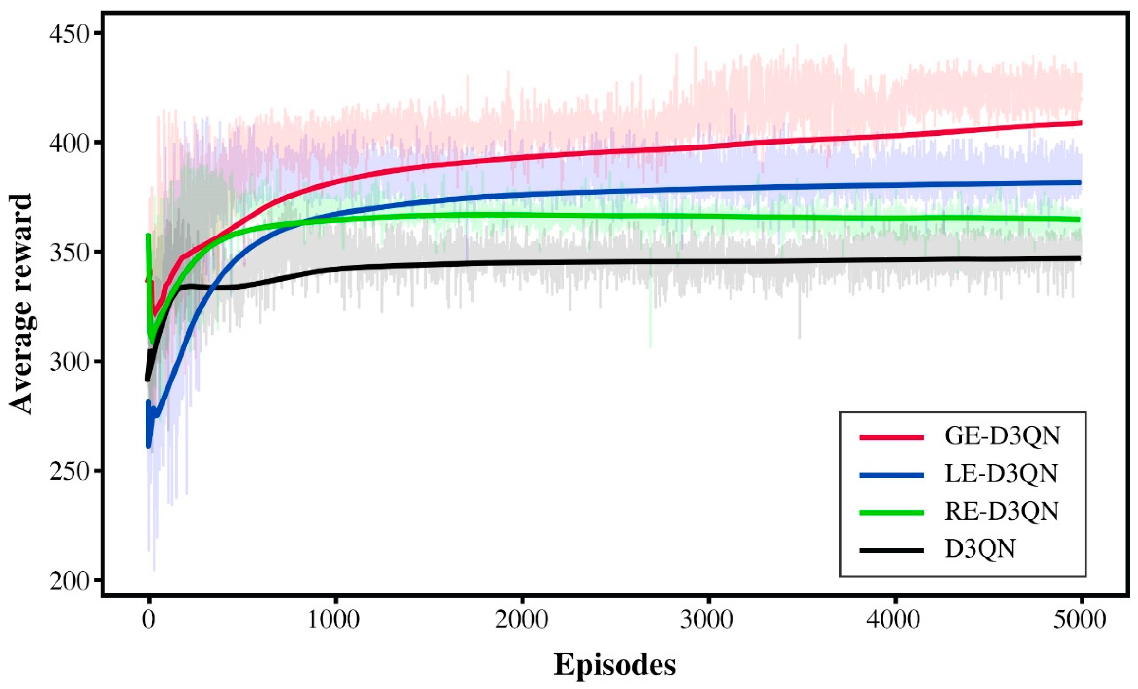
Figure 10 presents a comparison of the performance of four algorithms over 5000 episodes. The RE-D3QN and D3QN algorithms initially outperform LE-D3QN in learning efficiency but fail to enhance their exploration capability beyond 500 episodes. In contrast, the LE-D3QN algorithm starts with weaker performance but surpasses RE-D3QN and D3QN after 1000 episodes while maintaining its exploration capability. Overall, the GE-D3QN algorithm demonstrates the best training performance, effectively integrating dynamic ocean currents with observation tasks to achieve superior overall results.

Figure 11 illustrates the adaptive observation paths using the GE-D3QN algorithm in a dynamic ocean current background. As shown in the figure, AUV1, AUV2, and AUV3 depart from open waters, where most of the surrounding ocean currents align with their travel direction. The AUV platforms are able to effectively carry out observation tasks by utilizing the direction of the ocean currents. AUV4 and AUV5 are located in areas with more terrain obstacles and surrounding countercurrents. The AUV platforms can adjust their states based on the ocean currents, overcoming the constraints of the countercurrent zones and successfully performing observation tasks while avoiding collisions with the terrain.

Table 5. Comparison of performance metrics for the observation paths of four algorithms in ocean current environments.

Metrics	GE-D3QN	LE-D3QN	RE-D3QN	D3QN
Reward value	416	378	362	341
Average travel length	908.95 km	942.75 km	954.07 km	950.02 km
Average observation speed	7.51 km/h	7.69 km/h	7.88 km/h	7.76 km/h
Average travel time	121.05 h	122.58 h	121.12 h	122.45 h
Average reward value per hour	3.44	3.08	2.99	2.78
Average computational time	0.8522 s	0.9012 s	0.8363 s	0.8019 s

presents the evaluation results of various performance metrics for the observation paths of four algorithms in ocean current environments. After introducing the ocean current constraints, the observation strategies formulated by the four algorithms all improved the average observation speed of the AUVs compared to the initial speed (7 km/h), with increases of 7.29%, 9.86%, 12.57%, and 10.86%, respectively. This indicates that all algorithms are able to effectively utilize ocean current information to optimize the attitude angles of the AUVs, thereby improving observation efficiency.

Compared to the D3QN algorithm, the average reward per hour of RE-D3QN, LE-D3QN, and GE-D3QN increased by 7.55%, 10.79%, and 23.74%, respectively, demonstrating the superiority of recurrent neural networks in learning and utilizing ocean current information. Although D3QN exhibits the highest computational efficiency, it achieves the lowest rewards and falls short in terms of both travel distance and time compared to GE-D3QN. It is noteworthy that, while the observation strategy formulated by RE-D3QN achieved the fastest observation speed (7.88 km/h), its average travel length per task was the longest, resulting in only a 7.55% increase in the average reward per hour in the ocean environment. This suggests that a higher speed does not necessarily equate to better observation performance. Overall, GE-D3QN stands out with the shortest travel distance, optimal travel time, highest rewards, and acceptable computational time, making it particularly effective for devising observation strategies for AUVs in ocean current environments.

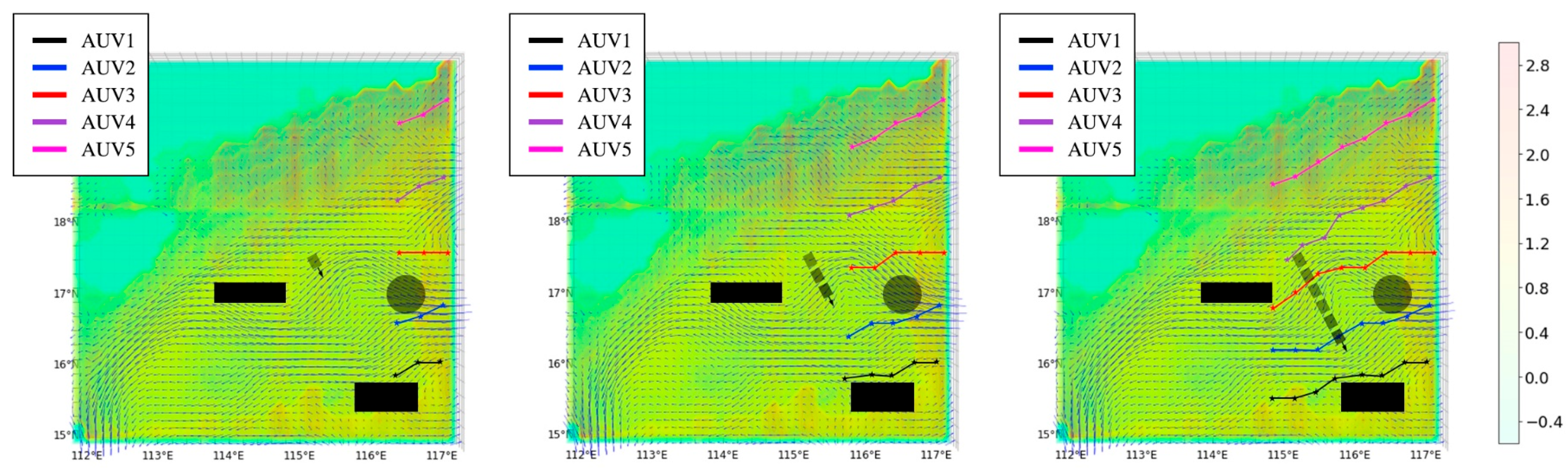
4.4. Scenario 3: Multi-AUV Observation Path Planning in Complex Marine Environments

Through the comparative experiments presented in Section 4.2 and Section 4.3, the superiority of the proposed GE-D3QN algorithm over LE-D3QN, RE-D3QN, and traditional D3QN algorithms has been validated. This section further demonstrates the applicability and effectiveness of the GE-D3QN algorithm in complex marine environments, including the influence of ocean currents and obstacles. In the experiment, the number of AUV platforms is set to five, with an initial navigation speed of 7 km/h. The initial positions of the AUVs are detailed in Table 4. The AUV platforms rely on onboard sonar systems to perceive their surrounding environment and autonomously avoid obstacles.

During marine observation missions, AUV platforms are not only influenced by seabed topography but also face potential threats from unexpected obstacles such as shipwrecks, large marine organisms, and other underwater military equipment. To enhance the realism of the simulation environment and better reflect actual ocean conditions, both static and dynamic obstacles are introduced in the observation area. For irregular static obstacles such as islands and reefs, a geometric modeling approach is employed, simplifying them into spherical and cuboid shapes. Spherical obstacles are used to reduce the complexity of modeling smaller irregular objects, while cuboid obstacles simplify the representation of larger irregular structures. Dynamic obstacles, such as ocean buoys and drifting objects, are modeled as cuboid obstacles moving in uniform linear motion. This approach ensures a more accurate simulation of real-world ocean scenarios, enhancing the algorithm’s adaptability to dynamic and unpredictable underwater environments.

As shown in Figure 12 and Figure 13, in complex marine environments, the multi-AUV systems based on GE-D3QN can sense obstacles in real time during the observation process and quickly adjust their strategies, selecting collision-free paths to efficiently collect ocean information. The analysis of how the observation strategy in such scenarios enhances the performance of the marine forecasting system will be further explored through the experiments presented in Section 4.5.

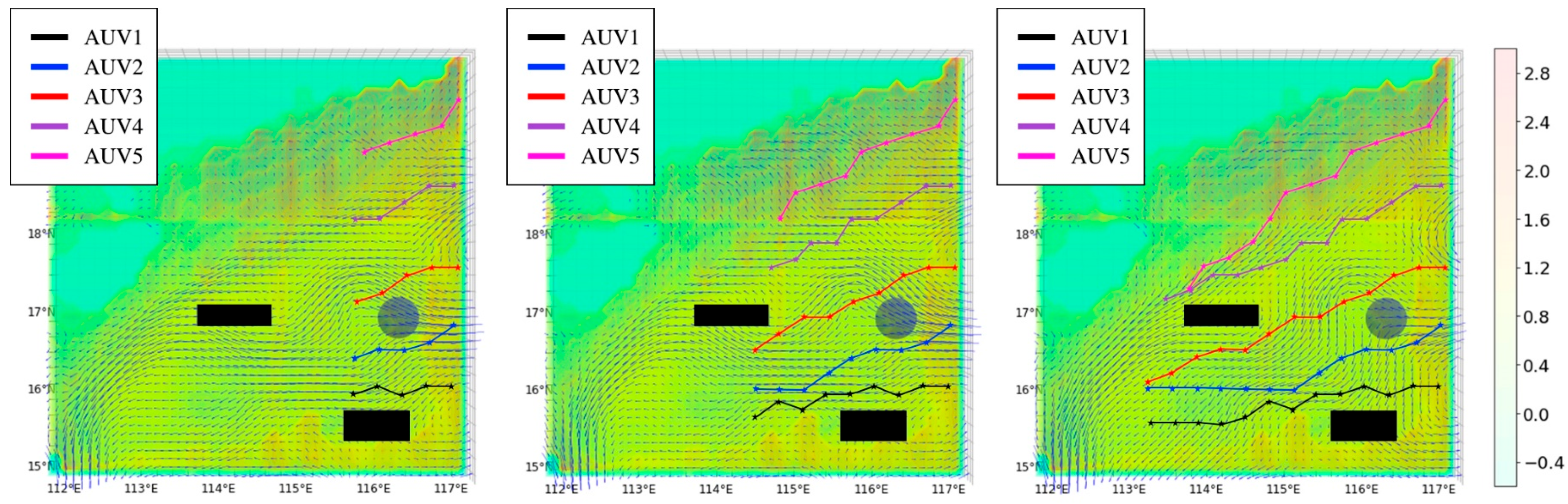
4.5. Scenario 4: Multi-AUV Observation Path Planning with Varying Numbers in Three Different Marine Environments

To further examine the impact of collaborative observations using different numbers of AUVs under the GE-D3QN algorithm on the performance of the marine environment numerical prediction system, we conducted comparative experiments using three, five, and seven AUVs in background fields without ocean currents, with ocean currents, and with both ocean currents and dynamic/static obstacles. The starting positions of the AUVs are detailed in

Table 6. Multi-AUV starting position settings.

Scenario	Platform	Starting Position
Three-AUV collaborative observation situation	AUV 1	[117° E, 19.5° N, 30th layer]
	AUV 2	[117° E, 17.5° N, 26th layer]
	AUV 3	[117° E, 15.5° N, 22nd layer]
Five-AUV collaborative observation situation	AUV 1	[117° E, 15.5° N, 30th layer]
	AUV 2	[117° E, 16.5° N, 26th layer]
	AUV 3	[117° E, 17.5° N, 22nd layer]
	AUV 4	[117° E, 18.5° N, 18th layer]
	AUV 5	[117° E, 19.5° N, 14th layer]
Seven-AUV collaborative observation situation	AUV 1	[117° E, 15.5° N, 30th layer]
	AUV 2	[117° E, 16.5° N, 26th layer]
	AUV 3	[117° E, 17.5° N, 22nd layer]
	AUV 4	[117° E, 18.5° N, 18th layer]
	AUV 5	[117° E, 19.5° N, 14th layer]
	AUV 6	[117° E, 15.5° N, 18th layer]
	AUV 7	[117° E, 17.5° N, 14th layer]

.

As shown in Figure 14, since all the experiments used the GE-D3QN algorithm, the reward curves exhibit similar fluctuations, plateauing around the 500th episode. With more agents, the seven-AUV scenario achieved the highest total reward due to increased data collection. However, in terms of average reward per AUV, the seven-AUV scenario performed worse, while the three-AUV scenario had the best observation efficiency. This suggests that while a greater number of AUVs enhances overall data collection, it does not necessarily improve the quality of individual observations. A smaller number of AUVs can yield more cost-effective data with lower resource consumption.

The assimilation technique processes observed data by integrating AUV path coordinates and collected sea temperature data into the assimilation system based on their respective layers. The RMSE between true and predicted values is then calculated, with the average RMSE across all layers representing the RMSE of the observation path. Data from observations by three, five, and seven AUVs were assimilated, and the experimental results are presented in

Table 7. RMSE comparison of sampling and assimilation results for different numbers of AUVs.

Scenario	Three AUVs	Five AUVs	Seven AUVs	Random
Environments without ocean currents	0.5324 °C	0.4939 °C	0.4883 °C	0.5841 °C
Environments with ocean currents	0.5431 °C	0.5103 °C	0.4924 °C	0.5845 °C
Environments with ocean currents and obstacles	0.5632 °C	0.5318 °C	0.5161 °C	0.6043 °C

.

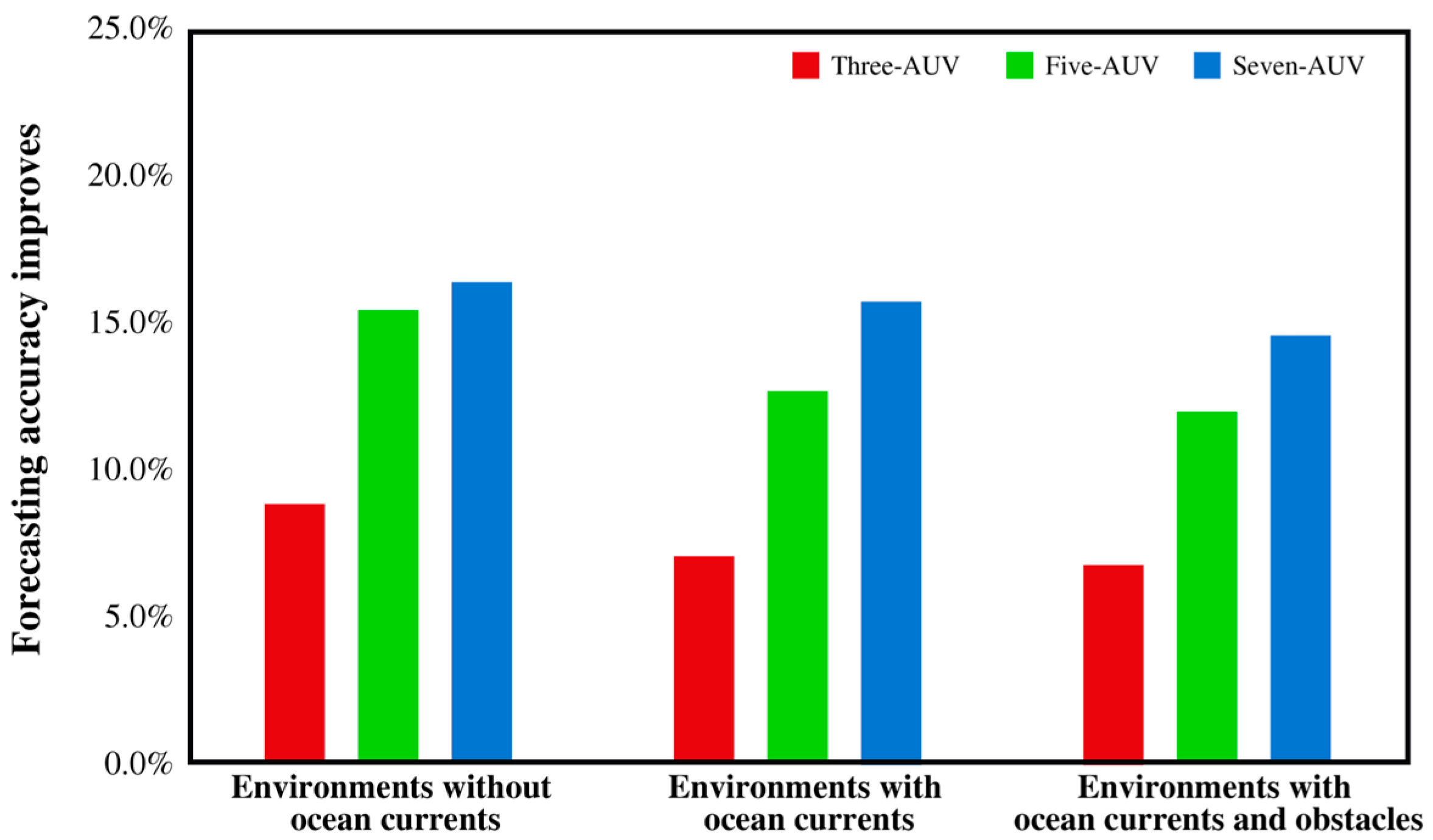
As shown in Table 7 and Figure 15, regardless of observation constraints, the seven-AUV experiment outperforms the three-AUV and five-AUV experiments in assimilation performance. The forecast accuracy improvements of the three-AUV experiment over random sampling are 8.851%, 7.083%, and 6.801%, respectively. For the five-AUV experiment, the improvements rise to 15.443%, 12.695%, and 11.997%, while the seven-AUV experiment achieves the highest gains at 16.401%, 15.757%, and 14.595%.

When AUVs operate without constraints, they achieve optimal observation performance, with steadily increasing reward values and minimal fluctuations. Introducing ocean current constraints forces the observation strategy to balance temperature gradients and energy consumption, prioritizing higher reward points within a limited time rather than maximizing observations at all costs. This leads to slightly lower reward values and a minor drop in assimilation performance across all three AUV formations. With both ocean currents and obstacles in the background field, the number of constraints increases, and obstacles may appear in high-gradient regions. To ensure observation safety, the algorithm avoids these areas, further reducing assimilation performance for all three AUV formations.

Moreover, increasing the number of AUVs from three to five improves the average RMSE of data assimilation experiments by 5.793% across all three background fields. However, increasing the number from five to seven yields only a 2.211% improvement, highlighting diminishing returns. While additional AUVs enhance data collection and assimilation accuracy, their marginal benefits decrease. Therefore, the number of AUVs should be optimized based on the required observation accuracy.

5. Conclusions

This study proposes an optimization method for multi-AUV adaptive observation strategies based on an improved D3QN algorithm. To address the challenges of tightly coupled environmental modeling and the difficulty of determining the optimal observation strategies in complex marine environments with traditional algorithms, we leverage the advantage of DRL algorithms, which autonomously interact with the environment to facilitate learning. The problem is formulated as a POMDP, and a DRL approach based on the D3QN framework is developed. To enhance the D3QN algorithm, we integrate a GRU network to overcome issues such as partial observability and the complexities of dynamic 3D marine environments. The main contributions are as follows: (1) The proposed method offers state-space prediction and rapid convergence, enabling AUVs to complete observation tasks efficiently while effectively leveraging ocean currents to reduce energy consumption and avoid unforeseen obstacles. (2) The simulation results demonstrate that the proposed GE-D3QN method significantly outperforms the D3QN, RE-D3QN, and LE-D3QN algorithms in complex marine environments, particularly regarding safety, energy consumption, and observation efficiency. (3) Experiments deploying three, five, and seven AUVs across three marine scenarios, combined with data assimilation analysis, reveal that while increasing the number of platforms improves forecasting accuracy, the improvement rate gradually diminishes, reflecting diminishing marginal returns. These findings validate the effectiveness and practicality of the proposed method for multi-AUV cooperative observation tasks.

Although this study has yielded promising outcomes, several limitations remain. First, under sparse reward conditions, achieving an optimal balance between team incentives and individual rewards is crucial for fostering effective collaboration among agents—a challenge that warrants further investigation. Second, extending the algorithm to larger-scale environments introduces significant issues in computational complexity and coordination, which will be a primary focus of our future work. Finally, validating the proposed algorithm in real marine settings is essential for confirming its practical applicability, and this remains a key objective for subsequent studies.