Article

An Exploratory Assessment of a Submarine Topographic Characteristic Index for Predicting Extreme Flow Velocities: A Case Study of Typhoon In−Fa in the Zhoushan Sea Area

1
College of Civil Engineering and Architecture, Zhejiang University, Hangzhou 310058, China
2
Second Institute of Oceanography, Ministry of Natural Resources, Hangzhou 310012, China
3
Ningbo Hangzhou Bay Bridge Development Co., Ltd., Ningbo 315033, China
4
Water Affairs Bureau of Jiujiang District, Jiujiang District, Wuhu 241001, China
*
Author to whom correspondence should be addressed.
J. Mar. Sci. Eng. 2025, 13(5), 864; https://doi.org/10.3390/jmse13050864
Submission received: 15 March 2025 / Revised: 15 April 2025 / Accepted: 15 April 2025 / Published: 25 April 2025
(This article belongs to the Section Coastal Engineering)

Abstract

:
This study analyzes the 96 h flow velocity time series data from the Zhoushan Sea during Typhoon In−fa to investigate the conditions for extreme flow velocities. Through force analysis of the unit fluid and statistical analysis of topographic features, we identified the critical water depth, slope, and sea surface width for extreme flow velocities under ideal conditions as 15 m, 4.5°, and 2000 m, respectively. The Submarine Topographic Characteristic Index (STCI) is introduced for the first time in this study, revealing its significant impact on extreme flow velocities. Three types of “extreme velocity points”—associated with constant storm surge, astronomical tide, and typhoon storm surge—were defined, occurring over 85% of the time during typhoon events. These extreme velocity points were analyzed in relation to their topographic characteristics, including water depth, slope, and sea surface width. Simulations of Typhoon In−fa in the Zhoushan Sea area were used to construct the STCI model, resulting in the following weightings: water depth = 0.96, slope = 0.39, and sea surface width = 0.49. Typhoon In−fa occurred in 2021, exhibited a maximum wind speed of approximately 35 m/s, and played a key role in the hydrodynamic processes investigated in this study. Validation with Typhoons Muifa (2021) and Bebinca (2413) confirmed the model’s high consistency. The STCI model provides insight into the occurrence of extreme velocities, categorizing them according to tidal phase and typhoon influence. Preliminary findings indicate the model’s applicability under varying typhoon intensities, offering a robust tool for predicting extreme seabed flow velocities during typhoon events.

1. Introduction

Typhoon storm surges, a significant extreme marine hazard, profoundly influence ocean flow velocity and direction. Understanding the conditions that lead to extreme flow velocities during these events is crucial for improving the accuracy of seabed engineering designs and enhancing disaster early warning systems.
In storm surge formation research, Resio emphasized the role of wind stress in water level rise, highlighting the strong correlation between surge severity, typhoon intensity, and trajectory [1]. Mofjeld demonstrated that the superposition of typhoon storm surges often leads to significant increases in extreme water levels and flow velocities, particularly during landfall events [2]. Westerink noted that the extent of storm surge impacts is not only driven by meteorological factors but is also strongly influenced by coastal topography, with complex terrains often amplifying the surge locally [3]. Recently, researchers have focused on the nonlinear coupling effects of typhoon storm surges. Gönnert, through numerical simulations, confirmed that such coupling significantly amplifies flow velocities and water levels, especially in narrow waterways and areas around islands [4].
Existing studies have primarily examined the effects of wind stress on surface ocean flow velocity and the coupling of typhoon storm surges with extreme flow velocities. However, the inherent seabed topographic conditions that contribute to extreme flow velocities remain underexplored. This study seeks to address this gap by investigating the effects of seabed topographic complexity on water flow patterns and velocity distribution. Gervais noted that shallow waters, narrow channels, and regions with smaller sea surface widths are particularly susceptible to extreme flow velocities, where topographic features significantly amplify the influence of wind stress and bottom friction on fluid motion [5]. Zhang’s model simulations further revealed that islands and seabed protrusions notably affect extreme flow velocities, with their impact being most pronounced in shallow waters [6].
To enhance understanding of the extremity of typhoon–storm surge−coupled flow velocities, the generalized extreme value (GEV) theory, as proposed by Coles, has become a standard tool in extreme event analysis [7]. Katz applied the GEV model to derive the statistical distribution of extreme flow velocities and water levels, demonstrating its effectiveness in predicting extreme velocities during typhoon storm surges [8]. Hamdi refined the parameter estimation methods within the GEV model, improving its accuracy for typhoon−storm surge events [9]. Recently, Giaremis proposed using a long short−term memory (LSTM) deep learning model to correct systematic errors in storm surge simulations. This method, applied to historical hurricane data, successfully enhanced water level forecasting accuracy during Hurricane Ian in 2022 [10].
This study introduces the Submarine Topographic Characteristic Index (STCI) as a novel tool for assessing regions prone to extreme flow velocities. By calculating critical conditions for extreme flow velocities, using iterative algorithms, and validating the results with data from two additional typhoons, this research aims to improve predictions of ocean flow velocity changes under extreme meteorological events. The findings provide valuable guidance for marine engineering, disaster prevention, and early warning systems.

2. Study Area, Numerical Model and STCI Model

2.1. Study Area

This study examines the seabed along the route of a submarine cable, employing a kilometer−based coordinate system for spatial reference (Figure 1). Note that the coordinates are derived by converting geographical coordinates via a custom Gauss projection with 121.5° E as the central meridian, which defines the origin for the X and Y values in km. For the offshore region (Figure 1a), the GEBCO global bathymetry dataset was used, offering a resolution of 30 s × 30 s (approximately 200 m). To enhance data accuracy, depth measurements at various points were interpolated using high−resolution nautical charts.
The Zhejiang coastal area, known for its intricate terrain featuring numerous islands, bays, and complex seabed topography, poses unique challenges. The region experiences irregular semi−diurnal tides with significant tidal ranges, which are particularly pronounced during typhoon−induced storm surge events. A finer−scale seabed grid was applied for the Qushan and Shengsi Islands, with a resolution of 100 m. These islands are located in the northern part of Zhejiang Province’s Zhoushan Archipelago, near the outer edge of the Yangtze River estuary. The waterways in this area are narrow, characterized by complex tidal currents, and water depths gradually transition from shallow coastal zones to the open sea, ranging from 0 to 80 m. The seabed topography is dominated by numerous islands, reefs, and shoals (Figure 1b), resulting in highly intricate hydrodynamic conditions (Figure 1c). For better visualization, the 3D seabed map adopts a perspective view with the x− and y−axes spanning approximately 40 km and 50 km, respectively, while the depth is limited to a maximum of 80 m. Note that the visual scaling prioritizes clarity over true proportions, enabling a clearer depiction of the seabed’s complexity.

2.2. Topographic Characteristic Factors

Seabed geographic features serve as critical indicators for characterizing the natural marine environment. Among these, water depth ( h ) is the most significant parameter, directly influencing the vertical distribution of water temperature, flow velocity, and hydrodynamic forces. Stratification within the water column exhibits distinct dynamic behaviors in shallow versus deep regions [11]. The slope ( θ ) represents the inclination of the seabed surface. Regions with steeper slopes often experience accelerated flow velocities and intensified erosion effects, highlighting their role in shaping hydrodynamic conditions and sediment transport [12]. The sea surface width, which measures the openness of the ocean surface, is defined as the distance between a specific study location and its nearest protruding sea surface obstacle. The sea surface width (W) is defined as the minimum horizontal distance from a given study point to the nearest protruding barrier (e.g., an island or coastal outcrop) at the sea surface. This parameter serves as an indicator of the degree of exposure of the water body to open sea conditions. A greater sea surface width suggests that the corresponding region is more exposed, thereby allowing wind stress to have a more pronounced effect on the water flow. Although termed ‘Width’, it is used in our model to capture the hydrodynamic influence of the local marine topography on the distribution of wind−driven forces. In regions with no significant protruding obstacles (e.g., open sea areas to the north or west), the sea surface width may exhibit abrupt transitions along vertical or horizontal lines. This phenomenon arises naturally from the uniform absence of obstacles in those directions, such as elevated points visible above the water (e.g., the yellow markers in Figure 2). This feature significantly influences the intensity of wind stress, tidal interactions, and fluid motion, shaping local hydrodynamic processes [13]. A representative seabed topography (Figure 2) was randomly selected to illustrate these geographic features. Collectively, these parameters—water depth, slope, and sea surface width—play a pivotal role in determining material transport and the dynamic behavior of the marine environment.

2.3. Submarine Topographic Characteristics

2.3.1. Topographic Feature Statistics

The actual distribution of the three submarine topographic features is presented in Figure 3, with the corresponding statistical results summarized in Table 1. Water depth demonstrates significant variation across the study area, with an average depth of approximately 19.86 m. The slope is predominantly gentle, with a maximum inclination of 4.45°, indicating that the seabed topography generally undergoes gradual changes.
For clarity, please note that in Figure 3a the x and y coordinates are defined with respect to the lower left corner of the offshore region (refer to Figure 1). Moreover, the region depicted with a depth of 70 m corresponds to land areas and has been intentionally re−colored to avoid misinterpretation as actual water depth data.

2.3.2. Topographic Classification

Unit Fluid Force Analysis

The force analysis of a unit fluid in a stratified environment is essential for understanding ocean flow dynamics. This analysis incorporates several major external forces: gravity, buoyancy, bottom friction, wind stress, pressure gradient force, Coriolis force, and viscous force (Figure 4). Combined with the Navier–Stokes equations (Equation (1)), these forces offer a comprehensive framework for describing fluid motion.
ρ 0 ( V t + ( V · ) V ) = P + μ 2 V + F e x t
where ρ 0 is the fluid density, V is the velocity vector, P is the pressure, μ is the dynamic viscosity coefficient, 2 V is the Laplacian operator representing viscous forces, and F e x t includes external forces such as gravity, Coriolis force, and wind stress.
In the vertical direction, the net force acting on a unit fluid due to gravity and buoyancy is typically zero, expressed as follows:
F g + F b = ( ρ ρ 0 ) g
where ρ is the density of the unit fluid. This balance commonly describes convection phenomena in stratified fluids.
The bottom friction force arises at the seabed and is proportional to the square of the velocity, becoming particularly significant in shallow waters. It is expressed as follows:
F f = ρ 0 C f U U 2 + V 2 h = C f ρ 0 V 2 h  
where h is the water depth, C f is the bottom friction coefficient (typically 0.003), and V is the velocity of the fluid. This force provides negative resistance, influencing flow velocity near the seabed.
Wind stress represents the shear stress exerted by wind on the water surface, predominantly affecting surface fluids. It is calculated as follows:
F w = τ w = ρ a C d W W x 2 + W y 2 = ρ a C d U w 2
where C d is the wind stress coefficient (typically 0.002), ρ a is the air density, and U w is the wind speed. This force significantly influences the velocity and motion of surface fluids.
The pressure gradient force, a primary driver of fluid motion, arises from pressure differences within the fluid. For a unit fluid, it is expressed as follows:
F p = P
where P represents the pressure gradient. This force is typically associated with tides and typhoon−induced surges and is generally small enough to be neglected in certain cases.
The Coriolis force results from Earth’s rotation and depends on flow velocity and geographic latitude. It is expressed as follows:
F c = 2 ρ 0 V Ω s i n ( ϕ )
where Ω is Earth’s angular velocity, and ϕ is the latitude. In the Northern Hemisphere, this force deflects fluid to the right, contributing to phenomena, such as the Ekman spiral.
Viscous force originates from the internal viscosity of the fluid, creating shear stress due to velocity gradients. For three−dimensional motion, it is represented by 2 V , as in Equation (1). In vertical motion, it is commonly expressed as ρ 0 v V h , where v is the dynamic viscosity coefficient, and V h represents the velocity gradient with respect to depth. The viscous force intensifies with larger velocity gradients.
In stratified environments, the complete force balance is represented by the extended Navier–Stokes equation, written as follows:
ρ 0 V a = ρ 0 ( V t + ( V · ) V ) = P + μ 2 V C f ρ 0 V 2 h + ρ a C d U w 2 + 2 ρ 0 V Ω s i n ( ϕ ) + v V h
This equation integrates all major forces, providing a comprehensive framework for analyzing fluid motion under complex conditions such as typhoon−induced storm surges.
The analysis presented in this section serves as the theoretical basis for understanding how fluid forces interact with seabed topography. While the specific formulas are not directly employed in subsequent calculations, they underpin the assumptions made in the development of the STCI model and provide critical insights into the flow−topography interaction mechanisms discussed in later sections.

Sea Area Classification

In the ocean, flow velocity varies with depth and can be categorized into three primary regions. In shallow water regions, flow velocity is primarily influenced by wind stress, with the wind field serving as the dominant driving force. During typhoon events, this region often experiences the highest flow velocities. In mid−water regions, the effects of various nonlinear forces become more complex, with the overlap of storm surge and astronomical tide velocities being most pronounced. This often results in higher flow velocities. In deep water regions, the vast water mass diminishes the impact of wind stress. Additionally, bottom friction causes momentum diffusion and energy dissipation, leading to a reduction in the overall vertically averaged flow velocity.
Typhoon storm surge velocities are primarily the result of the nonlinear coupling between storm surge and astronomical tide velocities [14]. Therefore, effective water depth, which reflects the varying impacts of storm surge and astronomical tides, can serve as a criterion for dividing seabed regions based on depth.
Under the influence of storm surges, wind stress predominantly affects shallow water regions. Although the direct impact of wind stress is largely confined to the upper 16.6 m (the Ekman layer), the momentum transferred into the surface layers gradually propagates downward through turbulent mixing and nonlinear interactions with tidal currents. Consequently, this indirect effect extends into deeper layers, which justifies the consideration of water depths up to 30 m in our analysis. The depth of the Ekman layer, governed by the Coriolis force, is used to characterize the effective range of wind stress. The criteria for partitioning can be determined by the structure of the Ekman spiral [15], where the layer thickness depends on wind stress, the Earth’s rotation rate (Coriolis parameter f ), and the fluid’s viscosity. The formula for the Ekman layer thickness is as follows:
D E k m a n = 2 v f
where v represents the kinematic viscosity of water, typically 10 6 m 2 / s . However, during the landfall of a strong typhoon, the eddy viscosity coefficient v t can be used to calculate the Ekman layer depth [16]. In such conditions, v t may reach 10 3   m 2 / s or even higher; for this study, v t is set to 10 2 m 2 / s . The Coriolis parameter f is given by: f = 2 Ω sin ϕ . For the study area near Zhoushan, Zhejiang, located at approximately 30° latitude, the Coriolis parameter is calculated as f = 7.29 × 10 5 s 1 . Thus, the Ekman layer depth is determined as D E k m a n = 2 × 10 2 7.29 × 10 5 16.6   m . This calculation indicates that below a depth of 16.6 m, the influence of wind stress significantly weakens. Therefore, for this study, a depth of 15 m is chosen as the boundary between shallow water and intermediate water zones.
Astronomical tidal forces primarily influence the water column through pressure gradient variations and tidal flows driven by Earth’s rotation. In this study, it is assumed that the impact of astronomical tides is relatively uniform throughout the entire water column. However, with increasing water depth, the amplitude and velocity of tidal flows also increase, significantly affecting the horizontal movement of seawater. To analyze the effect of water depth on astronomical tides, the shallow water wave theory [17] is applied to describe tidal wave propagation in the ocean. The propagation velocity c of tidal waves is given by the following:
c = g h  
where g is the acceleration due to gravity ( 9.81   m 2 / s ), and h is the water depth.
The tidal wavelength λ is proportional to the tidal period T and the wave speed c , expressed as follows:
λ = c T = T g h
For a typical semidiurnal tide, such as the M2 tidal wave, the period is approximately 12.42 h, equivalent to 44,712 s. By substituting this period into the formula for tidal wavelength: λ = 44,712 × 9.81   h , the wavelength for various seabed depths can be calculated. For instance: At a seabed depth of h = 10   m , the corresponding semidiurnal tidal wavelength λ is approximately 443 km. At h = 80   m , the wavelength λ increases to approximately 1253 km. In this study, a typical tidal wavelength of 800 km is selected for the seabed. Using the same formula, the corresponding water depth is calculated to be approximately 32.6 m. This indicates that below a depth of approximately 32.6 m, the influence of astronomical tides significantly diminishes. Based on this calculation, a depth of 30 m is selected as the boundary between intermediate and deep water zones.
In summary, the seabed is divided into the following depth zones based on the effects of wind stress and astronomical tides: shallow water zone (water depth of 0–15 m, primarily influenced by wind stress.), intermediate water zone (water depth of 15–30 m, where the effects of nonlinear forces such as storm surges and astronomical tides are most pronounced), deep water zone (water depth exceeding 30 m, where the influence of both wind stress and astronomical tides significantly weakens).

2.4. Numerical Model of Typhoon

To fit and evaluate the newly proposed Submarine Terrain Characteristic Index (STCI) with respect to extreme flow velocity, this study adopts and extends the validated Typhoon In−fa model for the Zhoushan sea area, developed in Delft3D V4.04.01 [18]. The model serves as a robust foundation for further complex expansions and analyses. At the Qushan and Sijiao observation stations, the storm surge water level fitting achieved a goodness−of−fit (R2) exceeding 0.96, while 91.44% of astronomical tide water level error data points fell within 10 cm. These results underscore the reliability of the model’s structure and parameter settings, which were applied in this study. While direct flow velocity validation was not explicitly conducted, previous studies have established that successful water level validation inherently reflects the model’s ability to reproduce flow velocity patterns due to their physical coupling. This provides a reasonable level of confidence in the model’s reliability for analyzing storm surge and tidal flow dynamics.
Using Delft3D, flow velocity simulations were conducted for Typhoon In−fa. To ensure model stability, the first 48 h of data (starting from 00:00 on 21 July) were excluded, focusing instead on the 96 h period from 00:00 on 23 July to 00:00 on 27 July. Three MATLAB data files were created to support the analysis. To meet the specific requirements of this study, the original dataset was refined and expanded through the following steps:
(1) Refinement of seabed topography data
High−resolution seabed topography data was refined using interpolation techniques based on high−resolution nautical charts. A grid of 392 × 467 coordinate points was established, ensuring coverage of the submarine cable route. The refinement process involved smoothing algorithms to minimize noise while preserving critical topographic features. This grid validated the generalized extreme flow velocity calculation formula and supported the development of a 3D refined nautical chart (Figure 1c) derived from the [392 × 467 × 1] seabed topography dataset. All modeling and calculations in this study were conducted using MATLAB (R2023a Update 2 (9,14.0.2254940)).
(2) Extension of time series data
The 96 h time series dataset (from 00:00 on 23 July to 00:00 on 27 July) was extended by incorporating pre− and post−typhoon periods using linear interpolation and resampling methods. This ensured comprehensive coverage of flow velocity dynamics while preserving temporal continuity, including the pre−, mid−, and post−typhoon phases. This extension ensures comprehensive coverage of flow velocity dynamics, resulting in a final coupled flow velocity data matrix of dimensions 392 × 467 × 96.
(3) Expansion of flow velocity vector data
Flow velocity vector data were expanded into three datasets: storm surge flow velocity, astronomical tide flow velocity, and typhoon storm surge coupled flow velocity. This was achieved using MATLAB to process vector components from the hydrodynamic model output, ensuring accurate representation of spatial and temporal variations. These flow velocity datasets, collectively represented as Val: [392 × 467 × 96], provide comprehensive vector flow velocity information, enhancing the accuracy of the predictive formula.
(4) Data cleaning
Advanced data cleaning involved removing outliers using the Z−score method [19] and filling missing data through Kriging interpolation [20]. These approaches were specifically chosen to address the characteristics of the Typhoon In−fa dataset, ensuring robust and accurate processing. The combination of these methods effectively preserved the spatial and temporal consistency of the data while enhancing its suitability for analysis. These cleaning techniques were specifically tailored to the Typhoon In−fa data, providing a robust and consistent dataset for further analysis.

2.5. Submarine Terrain Characteristic Index (STCI)

The parameters of depth, slope, and sea surface width were selected based on their well−documented influence on hydrodynamic processes. Depth significantly affects vertical stratification and flow velocity, with shallower regions often exhibiting higher velocities due to wind stress. Slope plays a crucial role in accelerating flow velocity, particularly in regions with steep gradients, by intensifying erosion and sediment transport. The sea surface width determines the openness of the marine environment, affecting the distribution and intensity of wind stress and fluid motion. These parameters collectively provide a simplified yet effective framework for modeling extreme flow velocities in various marine environments.
Referring to typical statistical characteristics of spatial patterns in submarine geographic information science, such as slope and proximity index [21], factors like water depth, slope, and sea surface width can be integrated into a comprehensive index through weighting. Each submarine terrain characteristic is first standardized into a dimensionless value using the following formula:
X n o r m a l i z e d = X X m i n X m a x X m i n
where X m i n and X m a x represent the minimum and maximum values of the given characteristic. The comprehensive Submarine Terrain Characteristic Index (STCI) is then calculated using a weighted formula. The weights ( α 1 , α 2 , α 3 , etc.) represent the relative importance of each characteristic in the overall STCI. The formula for the STCI can be expressed as follows:
S T C I n o r m a l i z e d = α 1 · h n o r m a l i z e d + α 2 · s i n ( θ ) n o r m a l i z e d + α 3 · W n o r m a l i z e d
(1) Water depth h is the most critical factor affecting flow velocity. A higher weight can be assigned to water depth (e.g., an initial value of α 1 = 0.7, reflecting its significant contribution to flow velocity). This value can later be fine−tuned by minimizing errors in numerical simulation data.
(2) W represents the width of the sea surface, a critical variable in determining flow dynamics and the interaction between water movement and seabed topography. Under the combined influence of wind stress and tidal currents, sea surface width also contributes noticeably to flow velocity, though to a lesser extent than water depth. A moderate initial weight can be assigned to sea surface width (e.g., α 3 = 0.5).
(3) The overall seabed slope θ is relatively gentle, and its influence on flow velocity is significant only in steep terrains. Therefore, a lower weight can be assigned to slope (e.g., α 2 = 0.2).
To evaluate the STCI, the following process is applied. First, extreme flow velocity values are calibrated based on their probability of occurrence to assess the severity of extreme events. Then, “constant extreme flow velocity points” are identified as points that persist for 85% of the typhoon duration and correspond to specific coordinates ( x , y ) , which form the basis for subsequent analysis. At these coordinates, water depth, slope, and sea surface width are extracted and recorded in a [392 × 467] data matrix. These extracted data are standardized using Equation (11), and the standardized data are used in weighted calculations within the STCI model. Finally, the STCI model is fitted using the optimization algorithm fmincon based on the standardized data for water depth, slope, and sea surface width.
The model employs a weighted average to comprehensively evaluate the influence of each submarine terrain characteristic and optimizes the weights α 1 , α 2 , α 3 to predict whether specific locations are prone to forming “constant extreme flow velocity points.” Results indicate that when the STCI value falls between 25 and 40, “constant storm surge”, “constant astronomical tide”, or “constant typhoon−induced coupled flow velocity extreme points” are likely to occur. Conversely, other STCI values (e.g., 70) are almost never associated with “extreme flow velocity”.
Once the weight coefficients α 1 , α 2 , α 3 are determined, the Submarine Terrain Characteristic Index (STCI) can be used as an indicator to evaluate flow velocity characteristics in specific regions. This index provides a novel method for seabed terrain classification and has potential applications in hydrological modeling, disaster risk assessment, and other related fields.

3. Theoretical Derivation and Verification of STCI

The typhoon storm surge coupled flow velocity is generated by the nonlinear coupling of storm surge and astronomical tidal velocities. To analyze this phenomenon, the extreme flow velocity values are first calibrated based on the probabilities of occurrence for the three flow types. Using Delft3D, the “constant extreme value distribution points” of Typhoon In−fa are identified. These points represent common flow types that persist for at least 85% of the typhoon duration. Subsequently, the terrain characteristic index is theoretically derived and statistically validated to determine the critical values of water depth, slope, and sea surface width corresponding to these constant points. These three primary terrain characteristics are extracted from the coordinates and time points where flow velocity exceeds the extreme threshold during the typhoon period. The extracted characteristics are then normalized, and the objective function is optimized using the fmincon algorithm. This optimization minimizes overlap among the STCI values for the three constant points, resulting in a universal STCI terrain characteristic index model. Finally, the STCI model is validated using data from Typhoons Muifa and Bebinca, which exhibit characteristics similar to Typhoon In−fa. This validation establishes the approximate STCI ranges for the three different flow velocities, providing a valuable reference for future research and disaster prevention efforts.

3.1. Distribution of Extreme Flow Velocity and “Constant Extreme Value Distribution Points”

The foundation of the generalized extreme value (GEV) distribution theory is rooted in extreme value theory, which states that for a set of independent and identically distributed random variables, the distribution of their maximum or minimum values converges to certain specific forms. In this study, the 96 h period from 00:00 on 23 July to 00:00 on 27 July is analyzed, with each hour representing a set of flow velocity data. The extreme flow velocity values from this dataset are modeled using the GEV distribution. Extreme value theory suggests that, regardless of the underlying distribution of flow velocity data, the distribution of the maximum values will converge to one of three types of extreme value distributions, collectively represented by the GEV distribution. These include the Gumbel, Fréchet, and Weibull distributions. Among these, the Gumbel distribution is most commonly applied in modeling flow velocity [22].
The GEV distribution provides a framework for deriving the probability of flow velocities exceeding normal ranges and for predicting the likelihood of extreme flow velocity events. The GEV distribution is expressed as follows:
f ( V ) = 1 σ e x p ( ( 1 + ξ V δ σ ) 1 ξ ) ( 1 + ξ V δ σ ) ( 1 + 1 ξ )
where δ is the location parameter, representing the mean flow velocity during the 96 h typhoon period. σ is the scale parameter, indicating the range of variation in the hourly extreme flow velocities, with larger σ values corresponding to broader changes in extreme flow velocities. ξ is the shape parameter, determining the probability of extreme events. Based on its value, the distribution is classified as Gumbel distribution, Fréchet distribution, and Weibull distribution. ξ = 0 represents Gumbel distribution, commonly used to model light−tailed extreme events, such as flow velocity and wind speed.
This study utilizes Delft3D to simulate flow velocity data for the entire typhoon duration. Extreme value analysis of the flow velocity data is performed to fit the three parameters ( δ , σ , ξ ) of the GEV distribution. These parameters are estimated using methods such as Maximum Likelihood Estimation (MLE) [23] and Probability−Weighted Moment (PWM) [24]. Once the GEV distribution is fitted, the probability of flow velocity exceeding a given threshold (e.g., n m/s) can be calculated as V n = n f V d V . Using the fitted GEV distribution, the likely extreme flow velocity values within the 96 h of Typhoon In−fa can be predicted. Additionally, the return period of extreme flow velocities, such as a 100−year event, can be calculated, providing critical insights for hydrodynamic modeling and disaster risk assessment.

3.2. Flow Velocity Numerical Simulation

3.2.1. Numerical Model Flow Velocity

Using Delft3D, three MATLAB data files were created to represent the 96 h period from 00:00 on 23 July to 00:00 on 27 July. These files include flow velocity data for the entire domain under three conditions: flow velocity due to storm surge V w i n d ( x , y , t ) , flow velocity due to astronomical tide V t i d e ( x , y , t ) , and flow velocity resulting from the coupling of storm surge and astronomical tide V c o u p l e d ( x , y , t ) 
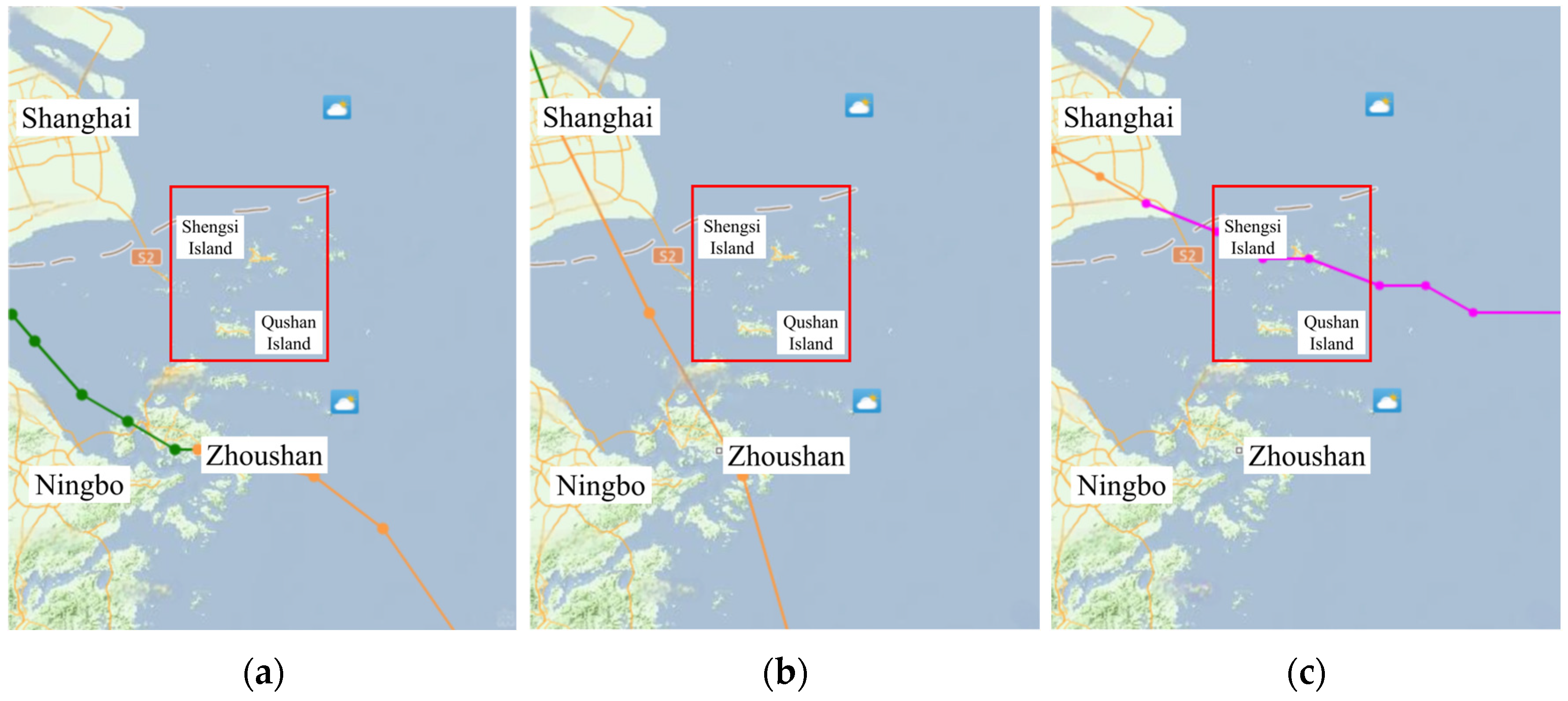
. At approximately 16:00 on 25 July, Typhoon In−fa reached the southeastern corner of the study area (Figure 5) and officially arrived between Shengsi Island and Qushan Island at 20:00. For further clarity, Typhoon In−fa reached a maximum wind speed of approximately 38 m/s, which results in an estimated wind stress of about 3.5 Pa (calculated using typical values for air density and the wind stress coefficient as described in Equation (4)). Furthermore, based on the adopted turbulent viscosity value of 10−2 m2/s, the Ekman depth is computed using Equation (8) to be approximately 16.6 m. These parameters were used in our numerical simulation to accurately represent the typhoon’s impact on the hydrodynamic processes of the study area. This time point, 20:00, is designated as the boundary for analyzing flow velocity across the entire domain. A four−hour interval before and after the typhoon’s arrival is typically used to examine the temporal variations of typhoon−induced storm surges [
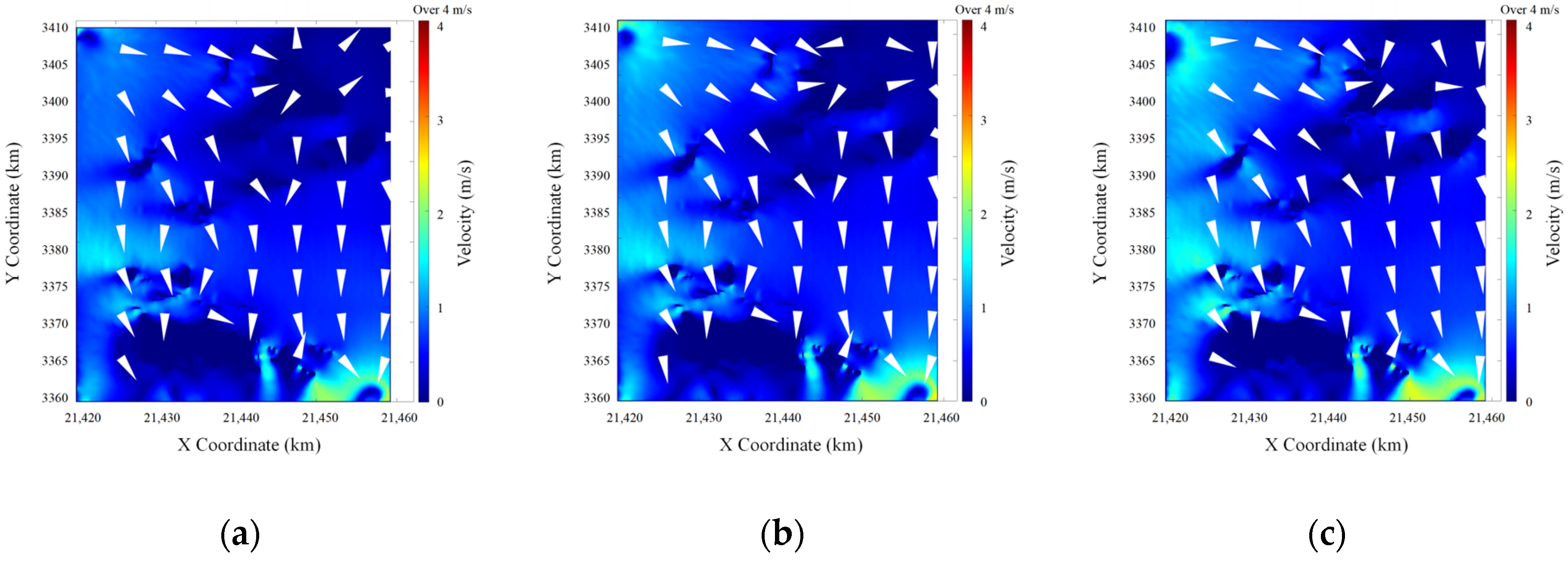
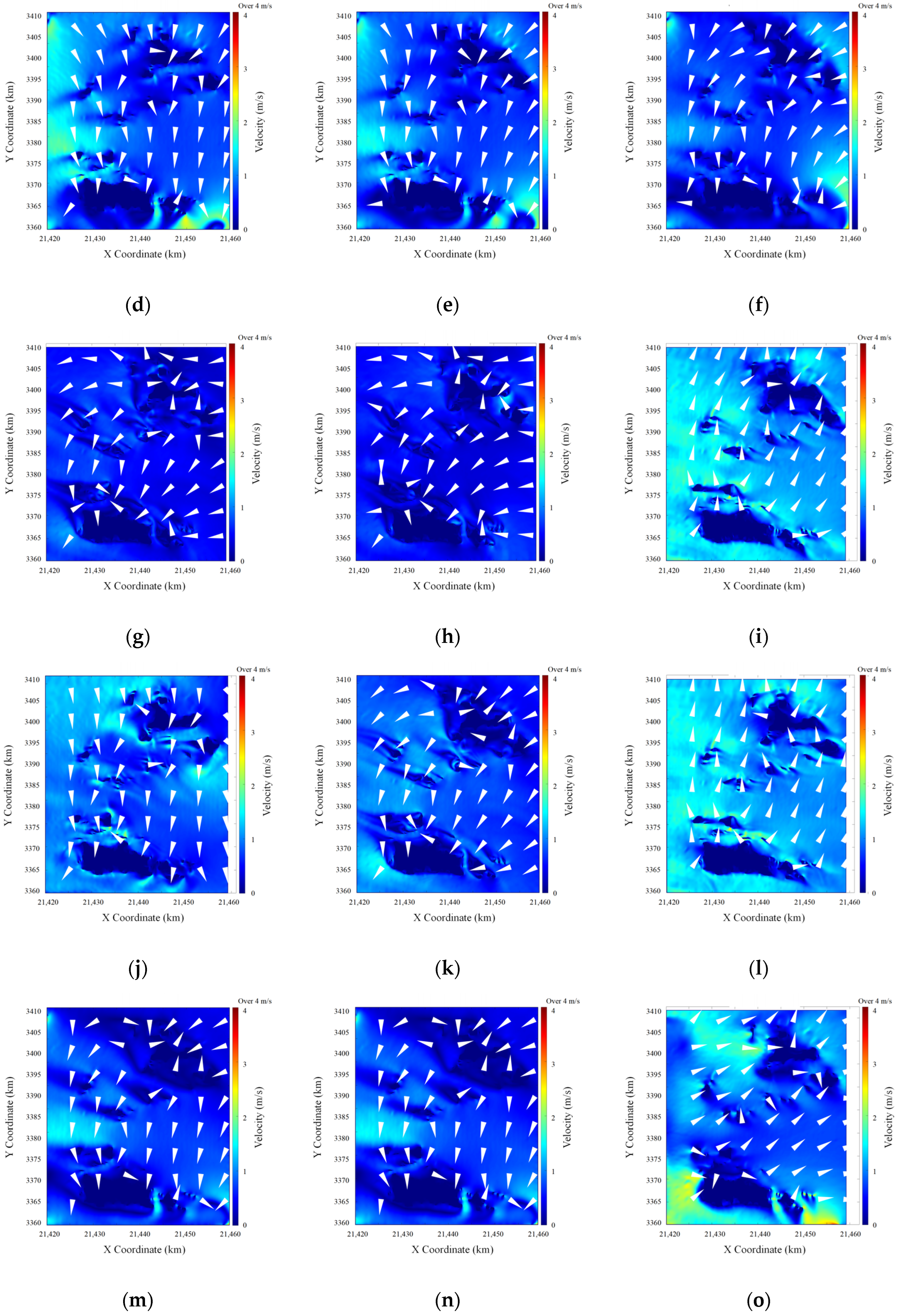
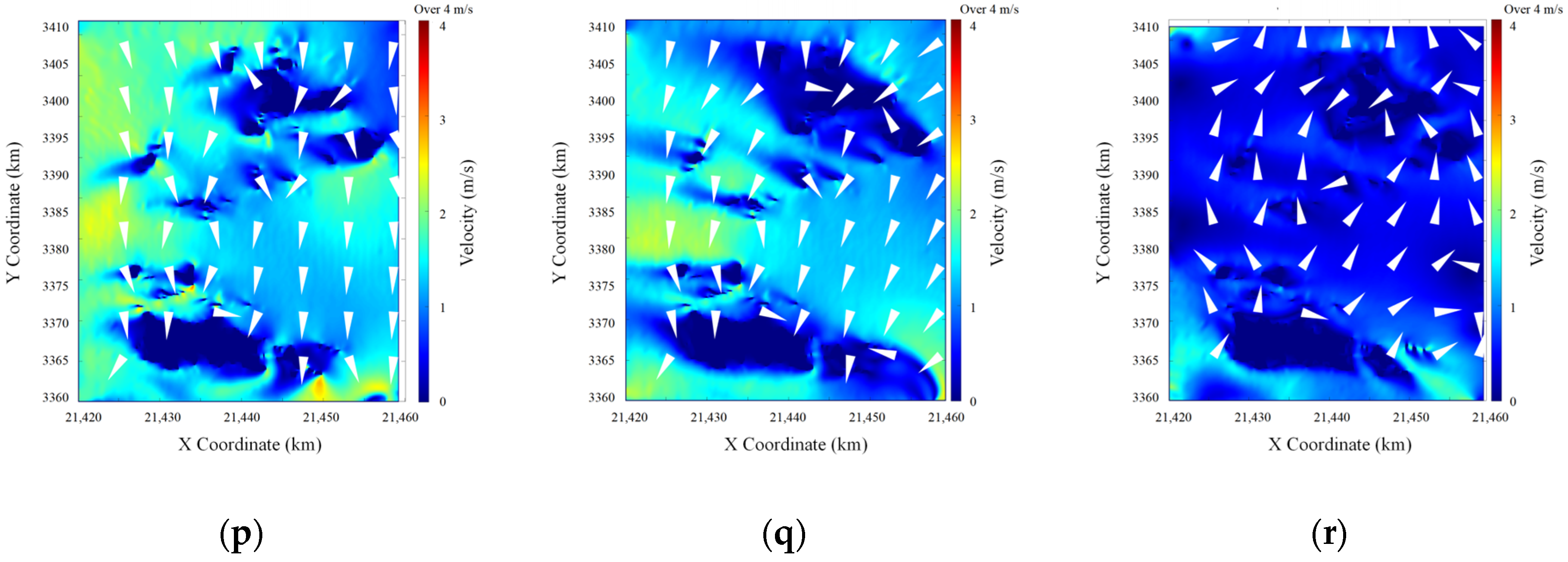
25]. Flow field maps at six selected time points—00:00, 12:00, 16:00, and 20:00 on 25 July, as well as 00:00 and 04:00 on 26 July—were extracted (Figure 5). By comparing these maps under the three conditions, the trends in flow velocity and direction were analyzed.
Under storm surge conditions, flow velocity intensifies significantly, especially along waterways and near the edges of islands, where strong vortices and accelerated currents are observed. These regions generally exhibit higher flow velocities due to the interaction of typhoon−induced forces with seabed topography. The flow direction during this period is heavily influenced by the typhoon’s path and tends to shift westward after the typhoon’s landfall. By contrast, under astronomical tide conditions, flow velocity and direction are primarily driven by tidal forces, showing more regular patterns. During tidal peaks, flow velocity increases notably in shallow regions and along waterways, reflecting the typical effects of tidal dynamics.
When storm surges and astronomical tides are coupled, the combined effects result in a predominant westward flow direction at the time of the typhoon’s landfall. In these conditions, flow velocity significantly intensifies in leeward areas of islands and along waterways, often exceeding the values observed under either storm surge or astronomical tide conditions alone. This amplification highlights the nonlinear interaction between storm surges and tidal forces, particularly in areas with complex seabed topography.

3.2.2. Statistical Analysis of Numerical Model Flow Velocity

Flow velocity data under pure storm surge, pure astronomical tide, and typhoon storm surge coupling conditions were statistically analyzed. Table 2 presents the seabed flow velocity characteristics for the entire 96 h time sequence from 00:00 on 23 July to 00:00 on 27 July, covering both the pre− and post−landfall periods of the typhoon. Table 3 provides statistical flow velocity characteristics specifically for the 48 h period during the typhoon, from 00:00 on 25 July to 00:00 on 27 July, focusing on the flow velocity trends before and after the typhoon’s landfall.
The maximum flow velocity under storm surge conditions reached 2.9 m/s, illustrating the powerful flow dynamics induced by storm surges under extreme weather conditions. The relatively high RMSE and MAE values observed are attributed to the significant influence of wind stress, as storm surges exhibit higher flow velocities and greater fluctuations in areas with an extensive sea surface width.
Astronomical tides played a crucial role throughout the typhoon period, particularly before the typhoon’s landfall at 20:00 on 25 July. During this period, ebb tides combined with northerly winds to produce strong flow velocities along the Zhoushan seabed. During the ebb tide phase prior to the typhoon’s arrival, intensified tidal outflows enhanced water movement, particularly in narrow waterways and around island peripheries, further amplifying the flow velocity to a maximum of 4.2 m/s. The coupled flow velocity of typhoon storm surges showed significant fluctuations, reaching a maximum of 5.5 m/s, which highlights the intense coupling effects of typhoon storm surges. These effects were especially pronounced during tidal peaks and ebbs, where the interaction of storm surges and tides led to extreme flow velocities.
After the typhoon made landfall, weakening wind speeds and the tidal transition into the flood phase resulted in reduced flow velocities, driven by the combined effects of astronomical tides and storm surges. As shown in Table 3, both the mean and maximum flow velocities after landfall decreased significantly compared to those before landfall. This aligns with the expected behavior during the passage of the typhoon’s eye: before landfall, the outer bands of the typhoon intensify wind speeds, while upon landfall, particularly in areas traversed by the eye, wind speeds drop sharply. Consequently, the maximum flow velocity recorded after landfall was 1.9 m/s.
During the typhoon, the mean and median flow velocities induced by astronomical tides were 1.12 m/s and 1.03 m/s, respectively, with relatively small fluctuations. This behavior is consistent with the tidal dynamics in the Zhoushan seabed area. After 20:00 on 25 July, as the tide transitioned into the early stage of flooding, the astronomical tide−induced flow velocities diminished, contributing to an overall reduction in tidal velocities.
Despite this, the coupling effect of the storm surge and astronomical tide partially mitigated the decrease in flow velocity after the typhoon’s landfall. As a result, the total flow velocity remained as high as 2.48 m/s. However, as the typhoon moved further away and the influence of the astronomical tide normalized, the flow velocity gradually stabilized.

3.2.3. Extreme Flow Velocity Statistics

The three data matrices generated by Typhoon In−fa—pure storm surge flow velocity, pure astronomical tide flow velocity, and typhoon storm surge coupled flow velocity (data structure: [392 × 467 × 96])—were organized and analyzed. The flow velocity data across the 96 h’ sequences were segmented to identify local extreme values within each time segment. These extreme values were then fitted using GEV theory, resulting in the shape ( ξ ), location ( δ ), and scale ( σ ) parameters that characterize the extreme value distributions.
To mitigate the influence of outliers on the distribution fitting, the top 2% of maximum values in each flow velocity dataset were removed. After filtering, the remaining 98% of the data were used for GEV distribution fitting. Table 4 presents the GEV distribution parameters and model performance metrics for the different flow velocity types, capturing the extreme value behavior under astronomical tide, storm surge, and typhoon storm surge conditions.
In terms of model performance, the root mean square error (RMSE) and mean square error (MSE) were used to evaluate the goodness of fit. Due to the periodic fluctuations of astronomical tides and typhoon storm surges, the RMSE values are relatively low at 0.223 and 0.224, respectively, indicating a strong fit. In contrast, the RMSE for storm surges is higher at 0.450, reflecting slightly lower fitting accuracy, which is consistent with the inherent uncertainty in wind direction and wind speed during storm surge events. Similarly, mean absolute error (MAE) results confirm the suitability of the GEV model for analyzing astronomical tides (non−typhoon conditions) and typhoon storm surge coupling (typhoon conditions).
The location parameter ( δ ) provides insight into the magnitude of extreme flow velocities. For typhoon storm surge flow velocities, δ = 0.725 , highlighting significantly higher extreme flow velocities in the region during typhoon events. In comparison, astronomical tide flow velocities have a lower extreme value, with δ = 0.695 . The scale parameter ( σ ) represents the degree of dispersion in the flow velocity distribution. For astronomical tides, σ = 0.282 , while for typhoon storm surges, σ = 0.326 . This indicates that flow velocity distributions exhibit greater variability during typhoon events compared to non−typhoon conditions, underscoring the pronounced changes in flow velocities during typhoon periods. The shape parameter ( ξ ) for all three flow velocity types is negative, indicating that the flow velocity distributions exhibit a right−skewed heavy tail. This characteristic is particularly evident for astronomical tides and typhoon storm surges, suggesting that their extreme flow velocities follow certain frequency patterns. In contrast, storm surges exhibit less regular flow velocity distributions. Consequently, the GEV model is most effective for analyzing the extreme values of astronomical tides and typhoon storm surges, making it a valuable tool for probabilistic analysis of extreme flow velocity events, see Table 5.
The probabilities of astronomical tide flow velocities and typhoon storm surge coupled flow velocities at different typical flow velocities reveal distinct distribution characteristics for these two flow types. For flow velocities exceeding 1.5 m/s, the probability is 3% for astronomical tides and 7% for typhoon storm surges. This aligns with the typical astronomical tidal dynamics observed in marine environments. Consequently, it is reasonable to calibrate the top 7% of coupled flow velocities as extreme flow velocities, with an extreme flow velocity threshold set at 1.5 m/s.
By focusing on flow velocities exceeding this defined threshold ( V   1.5 m/s), the probability of such events can be calculated using the extreme value distribution function f ( V ) (Equation (13)): P ( V 1.5 ) = 1.5 f ( V ) d V . Using this method, the probability of astronomical tidal flow velocities exceeding 1.5 m/s is approximately 3%, while for typhoon storm surge coupled flow velocities, the probability is about 7%. For safety and protection purposes, the higher probability value of 7% is selected as the extreme flow velocity occurrence probability. This emphasizes the importance of implementing protective measures to mitigate the risks associated with extreme flow velocities.
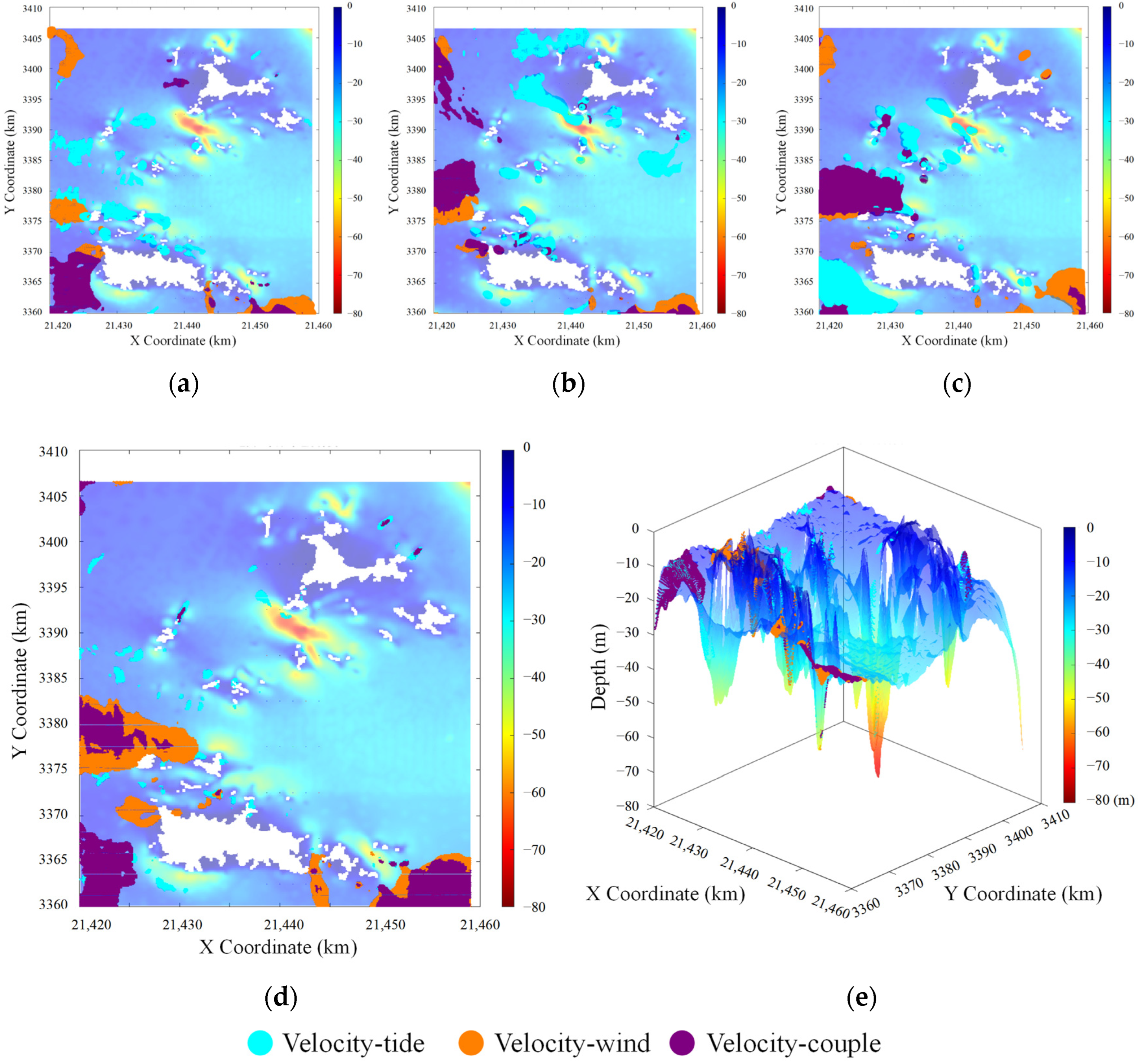
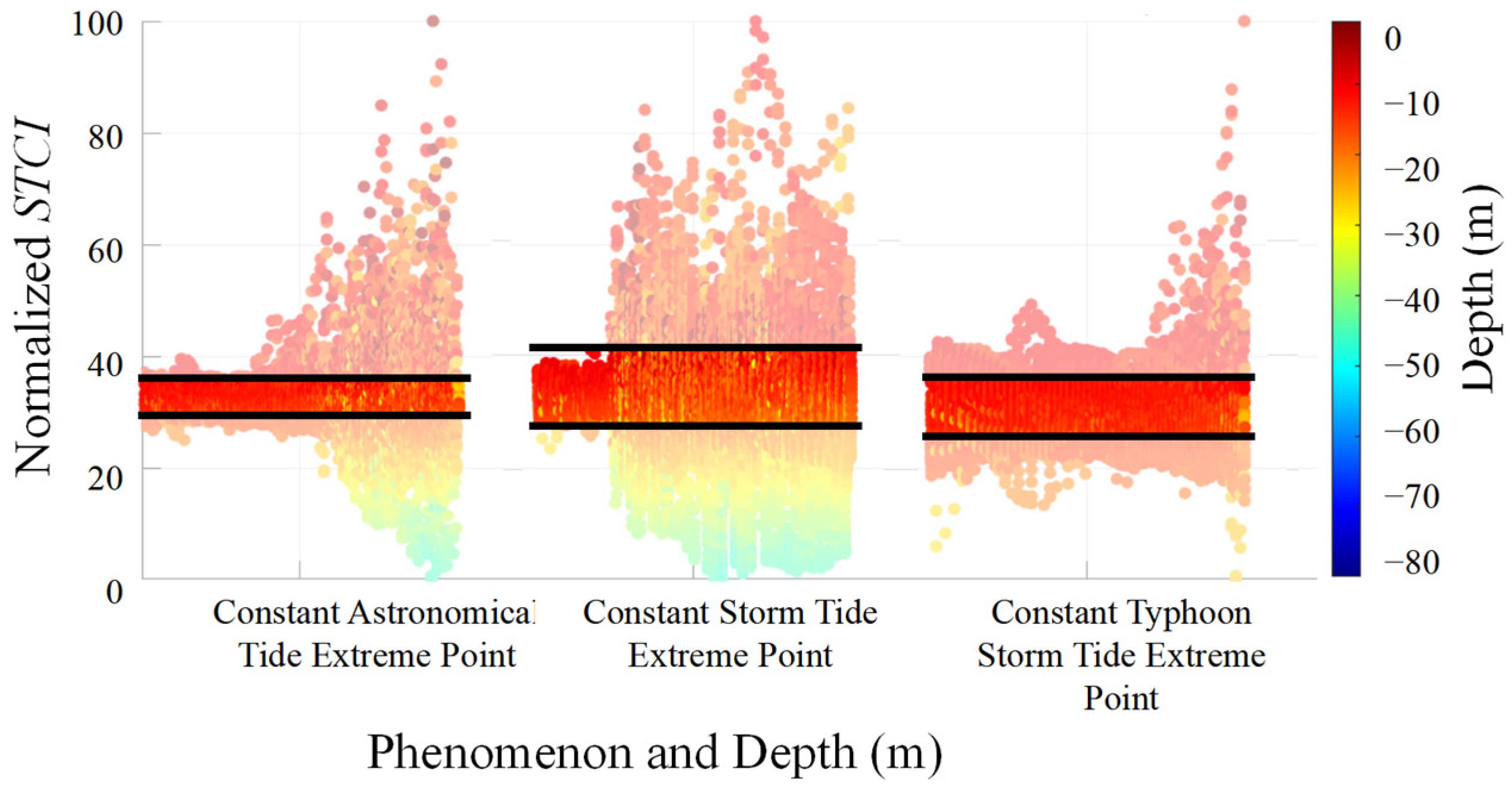
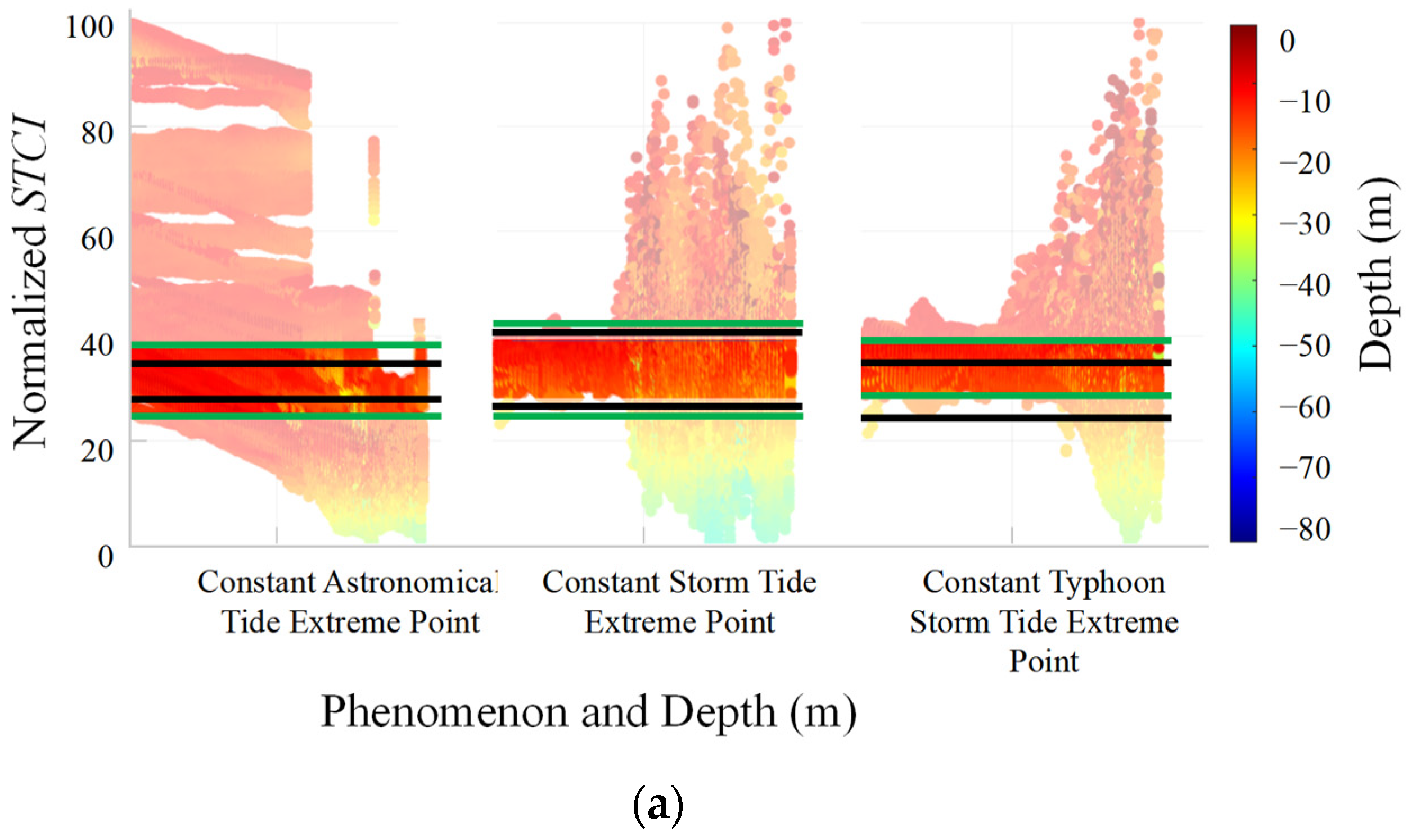
To better understand the distribution of extreme flow velocities, 3D visualization is used to display overlapping extreme values, representing all points with flow velocities exceeding or equal to 1.5 m/s for 82 h (85% of the typhoon period). Among the 392 × 467 coordinate points, those consistently exceeding the flow velocity threshold during these 82 h are marked on a unified 3D nautical chart and designated as “Typhoon In−fa Constant Extreme Flow Velocity Points”. A color−mapped visualization is employed to differentiate between the three flow velocity types, offering a clear and intuitive representation of the distribution of “constant extreme flow velocity points”.
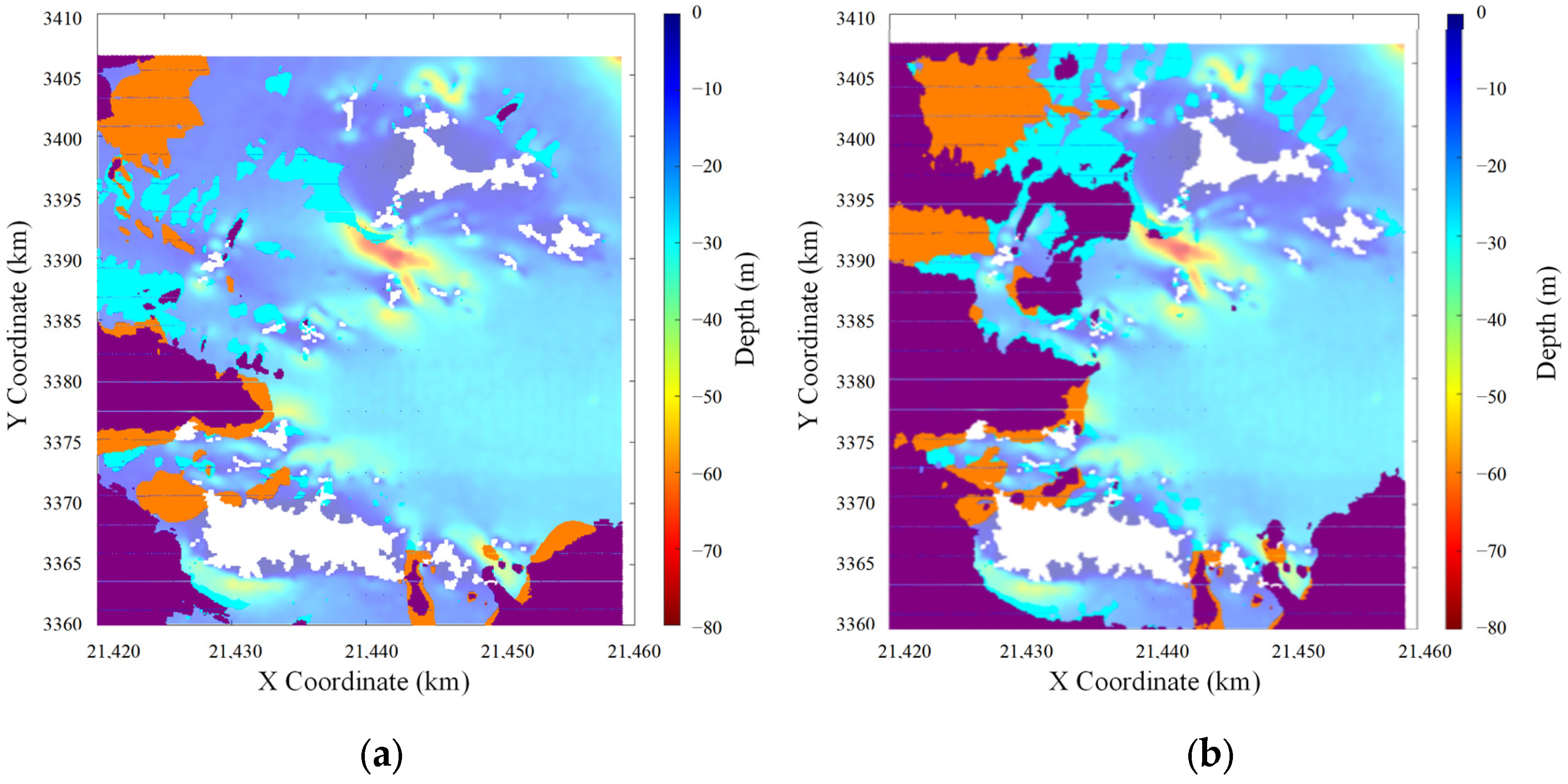
Figure 6a–c depict the distribution of extreme flow velocity points at three representative moments: 4 h before landfall, during landfall, and 4 h after landfall of Typhoon In−fa, respectively. These snapshots correspond to previously defined “Typhoon In−fa Constant Extreme Flow Velocity Points” and serve as case studies within the 85% typhoon period. 
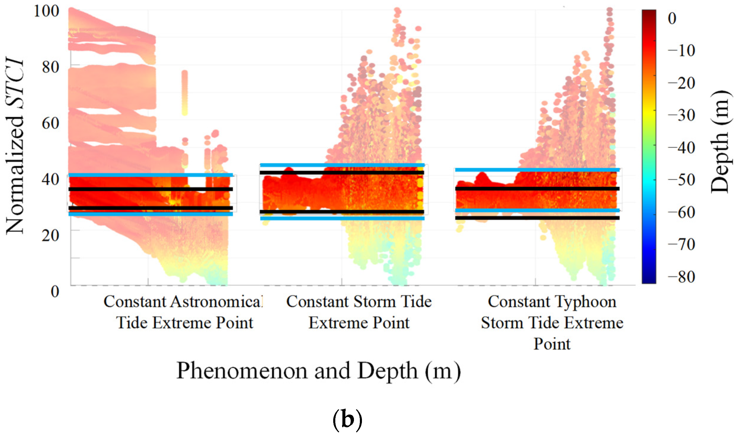
Figure 6d provides an overall view of the distribution characteristics of the “constant extreme flow velocity points” throughout 85% of the typhoon period, demonstrating that these extreme values are closely related to water depth, slope, and sea surface width.
The “constant storm surge extreme flow velocity points” of Typhoon In−fa (Figure 6d) are primarily concentrated in nearshore areas, shallow water zones, and the leeward sides of islands, where wind stress exerts a significant influence. Extreme flow velocities are notably higher in island regions, especially in wake zones, where velocities can exceed 3 m/s. As water depth increases, extreme flow velocities gradually decrease due to the diminishing effects of wind stress, which is most pronounced in shallow water areas. Although wind−induced velocities typically decrease with depth due to the exponential attenuation of wind stress, local topographic effects and the constructive coupling between tidal currents and storm surge can lead to secondary enhancements of the flow. In some regions, this results in relatively higher velocities even at depths beyond 30 m, where interference and channeling effects become significant. These localized phenomena do not contradict the overall decay trend but rather highlight complex hydrodynamic interactions in the study area.
The distribution of astronomical tide extreme flow velocity points is relatively uniform but sparse, concentrated primarily in intermediate water zones. Here, extreme flow velocities are largely driven by periodic tidal flows, with weak bottom friction in intermediate zones allowing the tidal energy to disperse smoothly. In other depth regions, “constant astronomical tide extreme flow velocity points” are almost nonexistent. In deeper waters, astronomical tide−induced flow velocities tend to stabilize, with overall velocities remaining low and peak values typically below 2 m/s.
The “constant typhoon storm surge coupled extreme flow velocity points” exhibit more complex distribution characteristics. As indicated by the purple points, most extreme velocities occur in narrow waterways within shallow water zones, with some extending into intermediate water zones. In areas with relatively small sea surface widths, extreme velocity points are widely distributed. Near islands and in shallow waters, coupled extreme flow velocities can exceed 3 m/s, while in deep water zones, the extreme flow velocities stabilize as the influence of wind stress and topographic features diminishes.
Across all three flow velocity types, extreme values decrease and stabilize with increasing water depth. While astronomical tide velocities exhibit a more uniform distribution in deeper water zones, the extreme values of storm surges and typhoon storm surges are concentrated in shallow water areas. Extreme flow velocities from storm surges and typhoon storm surges are concentrated in regions with complex seabed topography and steeper slopes, particularly in narrow waterways, around islands, and on the leeward sides of islands. In these areas, localized seabed topography amplifies wind stress effects, leading to significantly higher extreme flow velocities. In areas with small sea surface widths (0–4 km), especially near islands and coastal zones, extreme flow velocities are markedly higher. Conversely, in areas with larger sea surface widths (6–10 km), wind energy dissipates more effectively, resulting in an almost complete absence of extreme flow velocity points.

3.3. Terrain Corresponding to Extreme Flow Velocities

3.3.1. Typhoon Storm Surge Coupled Flow Velocity

Under the influence of pure wind stress, the shear stress exerted by wind on the sea surface directly affects the fluid’s surface layer. Momentum is transferred downward through friction, gradually influencing the middle and bottom layers of the fluid. This process leads to the formation of the Ekman spiral, derived from the Navier–Stokes (N−S) equations in a rotating coordinate system. Assuming horizontal wind stress and wind stress perpendicular to the water surface, the current velocity exhibits a spiral variation with depth.
Equation (14) describes the exponential decay of fluid velocity with depth under the influence of wind stress, accompanied by a rotation in flow direction. The Ekman depth ( D E k m a n ) is derived from Equation (8), where V w i n d 0 represents the velocity under maximum storm surge conditions, and ϕ is expressed in radians, written as follows:
V w i n d ( z ) = V w i n d 0 c o s ( z D E k m a n + ϕ ) e x p ( z D E k m a n )
Under the influence of tidal forces, the variation of tidal wave velocity with time and depth can be derived from shallow water wave theory. Simplifying the horizontal motion of the Navier–Stokes (N−S) equations, the tidal fluctuation formula is expressed as Equation (15).
V t i d e ( z ) = V t i d e 0 c o s ( ω t + ϕ )   e x p ( z D t i d e )
where ω represents the tidal frequency, D t i d e is the characteristic depth of astronomical tides, determining the decay of tidal velocity with depth, and V t i d e 0 is the velocity under maximum astronomical tide conditions.
When wind stress and astronomical tides act simultaneously, this study makes a simplified assumption that the flow velocity can be estimated through the linear superposition of wind−induced and tidal flow velocities. The resulting flow velocity ( V C o u p l e ( z , t ) ) is described in Equation (16).
V C o u p l e ( z , t ) = V 0 [ c o s ( ω t + ϕ )   e x p ( z D t i d e ) + e x p ( z D E k m a n ) c o s ( z D E k m a n + ϕ ) ]
where V 0 represents the surface layer flow velocity. To further quantify the influence of the phase difference between the tidal current and wind−induced motion on the maximum current, it derives a supplementary analytical expression under specific initial and boundary conditions. Assuming that at time t = 0 the tidal and wind−induced velocities are in phase (i.e., ϕ = 0) and setting the known maximum surface velocity as V 0 , the maximum current, V m , can be approximated by V m = V 0 [ e x p ( z D t i d e ) + e x p ( z D E k m a n ) ] , where z is the depth at which the combined effect reaches its maximum. In a sample numerical scenario, taking D t i d e = 32.6 m, D E k m a n = 16.6 m, and V 0 = 0.5 m/s, the computed maximum current is approximately 3.5 m/s. This expression explicitly demonstrates how the phase relationship and the exponential decay of water particle motion with depth contribute to the overall current profile. This formulation is a first−order approximation, and future work will aim to derive more rigorous integral formulations with mesh refinement (grid size tending to zero).

3.3.2. Critical Water Depth

To estimate the extreme flow velocity at different water depths, it is necessary to derive the velocity equation with respect to the variables influencing the flow velocity and identify their critical points. The Seafloor Topography Characteristic Index (STCI) explicitly identifies water depth, slope, and sea surface width as the core variables affecting flow velocity. By calculating the derivatives for each of these three variables, the conditions under which the flow velocity reaches its extremes can be determined, and the theoretical extreme flow velocities under these conditions can be computed. Under fully idealized conditions that exclude external forces, these results may differ from numerical modeling outcomes. However, they provide a qualitative description of the critical points for extreme values.
In shallow water regions, the primary influences are typhoons and shallow water wave theory. Due to the limited depth, wind stress significantly impacts the surface water layer, and tidal forces can also be rapidly transmitted through shallow water waves. Equation (14) applies to surface water in shallow regions, where the vertically averaged flow velocity for Z = 0 15   m is calculated as follows:
V a v g = 1 h 0 h V w i n d ( Z ) d Z = 1 15 0 15 0.5 e x p Z 15 c o s Z 15 + π 6 d Z 0.369   m / s
where V 0 = 0.5   m / s is the initial flow velocity induced by wind stress, D E k m a n = 15   m is the Ekman layer depth, and ϕ = π 6 is the phase angle. It should be noted that the above expression is an empirical representation aimed at capturing the average behavior of the wind−induced surface velocity in shallow water. It acknowledges that a more rigorous analytical formulation would account for the dependence of water particle motion on the wave period (or wavelength). In classical wave theory, the amplitude of water particle oscillations decays exponentially with depth with a decay rate that is a function of the wavelength; hence, at the same depth, different wave periods result in different amplitudes. Our current formulation does not include these effects explicitly and is intended as a simplified model.
In mid−depth water regions, the combined effects of wind stress and astronomical tides are observed. In this region, the influence of wind stress gradually weakens, while the impact of astronomical tides becomes more significant. Equation (16) represents the coupled flow velocity equation for storm surges, where the vertically averaged flow velocity for Z = 0 30   m is calculated as follows:
V a v g = 1 h 0 h V c o u p l e ( Z ) d Z = 1 30 0 30 0.5 e x p Z 30 c o s Z 15 + π 6 d Z 0.356   m / s
Similarly, the above expression for the mid−depth region is also empirical. It recognize that an accurate description of the hydrodynamic process should incorporate the impact of the wave period on the decay of water particle motion with depth. In practice, the exponential decay factor in a wave field is sensitive to the wavelength, and different wind wave periods would produce varying decay rates. Our current model does not capture these nuances; it represents a simplified approximation. Developing an analytical formulation based on energy considerations and wave dynamics is beyond the scope of the present study but is an important subject for future research.
In deep water regions, the primary influence comes from astronomical tides, while the impact of wind stress is minimal. The vertically averaged flow velocity for Z = 0 80   m is calculated as follows:
V a v g = 1 h 0 h V c o u p l e ( Z ) d Z = 1 80 0 30 0.5 e x p Z 30 c o s Z 15 + π 6 d Z 0.133   m / s
By deriving flow velocities at different water depths and excluding other external influences, it is observed that flow velocity is highest in shallow water regions, decreases in mid−depth regions, and is lowest in deep water regions. This magnitude relationship provides a qualitative basis for ranking flow velocities across the three regions and illustrates how the varying intensities of wind stress and astronomical tides shape flow dynamics at different depths.

3.3.3. Slope Critical Point

The influence of slope θ on flow velocity originates from gravitational acceleration, with V 0 still representing the initial flow velocity. The steeper the slope, the faster the flow velocity. For a downslope with an angle θ , a unit fluid experiences a resistive force F f due to friction with the slope surface. This frictional resistance is calculated using the bottom friction coefficient C f , which is 0.003, and is expressed as F f = C f m g c o s θ . In the downslope direction, the equation of motion for the unit fluid becomes: m a = m g s i n θ C f m g c o s θ . From this, the acceleration a of the unit fluid along the slope is derived as follows:
a = g s i n θ C f c o s θ
For a slope of unit length L , the velocity V s l o p e of the unit fluid at the bottom of the slope can be calculated as follows using the uniformly accelerated motion equation:
V s l o p e 2 = V 0 2 + 2 a L
Substituting the expression for a , the slope−induced velocity is given by the following:
V s l o p e = V 0 2 + 2 g ( s i n ( θ ) C f c o s ( θ ) ) L
This shows that the slope θ always impacts flow velocity, with steeper slopes generating higher velocities. By differentiating Equation (22) with respect to θ , the critical points of flow velocity can be determined as follows:
d V s l o p e d θ = g L ( c o s ( θ ) + C f s i n ( θ ) ) V 0 2 + 2 g ( s i n ( θ ) C f c o s ( θ ) ) L
Since this study focuses on seafloor slope angles ranging from 0° to 4.5°, the flow velocity at θ = 4.5° is considered the maximum. This analysis confirms that greater seafloor slopes result in higher flow velocities. The slope−induced flow velocity V s l o p e is found to be approximately 100% to 105% of the initial velocity V 0 , demonstrating the critical role of slope in influencing flow velocity in areas with steeper gradients.

3.3.4. Sea Surface Width

The concept of sea surface width W , newly introduced in this study, serves as a key parameter in describing factors influencing extreme flow velocities. While a definitive formula for deriving its critical value has yet to be established, statistical analysis of W provides valuable insights into its role in extreme flow dynamics. By examining the sea surface width W at “constant extreme flow velocity points”, it becomes possible to identify the conditions that favor the occurrence of extreme flow velocities. These insights offer a foundation for future derivations of critical values and contribute to a deeper understanding of the mechanisms driving extreme flow velocities in marine environments.
The characteristic parameters of water depth (15 m), slope (4.5°), and sea surface width (2000 m) were selected based on statistical analysis and preliminary simulations. While these values do not explicitly include the dependence on wave period, they are representative averages for the study area under the considered conditions. Future improvements will focus on integrating energy−based analytical formulations that account for the ratio of depth to wavelength.

3.3.5. Statistical Analysis of Topographic Critical Points

To further validate the critical points of geographic features corresponding to “constant extreme flow velocity points”, a statistical analysis was conducted based on three geographic factors. The extreme flow velocity points under the influence of storm surges, astronomical tides, and typhoon storm surges were treated as key nodes. These were analyzed in conjunction with geographic features such as water depth, slope, and sea surface width. The statistical analysis was based on the three types of extreme flow velocity points shown in Figure 6d (as shown in Table 6).
This study calculates the theoretical critical extreme water depth as 15 m and the slope as 4.5 degrees. The sea surface width, as an original concept, currently lacks a definitive formula for deriving critical values. According to statistical data, the extreme flow velocity of storm surges occurs at the shallowest depth of 13.33 m, which is related to the enhanced influence of wind stress on surface waters in shallower areas.
The constant extreme flow of astronomical tides corresponds to critical topographic conditions that differ from those of storm surges. The extreme points for astronomical tides appear at a greater depth of 16.67 m, indicating that tidal forces have a more significant impact in deeper waters. Additionally, compared to storm surges, astronomical tides can effectively influence water flow even in regions with gentler slopes, reflecting the broader and more consistent influence of tidal forces across all sea areas during both typhoon and non−typhoon periods. The sea surface width associated with astronomical tides is much larger than that of storm surges, suggesting that the extreme points for astronomical tides are more likely to occur in relatively open sea areas.
The constant extreme flow velocity point after coupling typhoon storm surges has a critical water depth of 15.89 m, a moderately steep critical slope, and a moderately sized critical sea surface width of 2128 m. Compared to storm surges and astronomical tides, the water depth, slope, and sea surface width of typhoon storm surges lie between those of the other two flow velocities.
The topographic features of these three extreme flow velocities generally align with the theoretically calculated critical points and the qualitative analysis in Section 3.2.3. Therefore, the characteristic parameters for extreme flow velocities are determined as follows: water depth—15 m; slope—4.5 degrees; and sea surface width—2000 m. These values were preliminarily selected based on energy dissipation considerations. In shallow water regions, a critical water depth of 15 m approximately marks the depth at which the energy input from wind stress and the wave−induced energy dissipation intersect significantly. Moreover, the dependence of water particle oscillations on wind wave periods—through the depth−to−wavelength (or period) ratio—was qualitatively evaluated, supporting this choice. Similarly, a slope of 4.5° and a sea surface width of 2000 m were determined by analyzing the rate of momentum transfer and energy dispersion in the marine environment.

4. Results and Discussion

4.1. STCI Values of Constant Extreme Flow Velocities

Based on Figure 6d, the coordinates corresponding to the “constant astronomical tidal extreme flow velocity points” (cyan), “constant storm surge extreme flow velocity points” (orange), and “constant typhoon storm surge coupled extreme flow velocity points” (purple) were extracted. The corresponding water depth, slope, and sea surface width values were identified and stored as ( d e p t h , s l o p e , w i d t h ) in a [392 × 467] data matrix, with ( x , y ) as the coordinate format. Within the study area, the constant extreme flow velocity points exceeding the set threshold of 1.5 m/s were found to be as follows: 13,332 points for storm surges, 12,242 points for astronomical tides, and 24,326 points for coupled flow velocities.
Based on Equation (12), this study employs the optimization algorithm fmincon to calculate the optimal weights α 1 , α 2 , α 3 , assigning different influence levels to water depth, slope, and sea surface width, respectively, to optimize the classification of phenomena. The optimization objective function in fmincon minimizes the overlap of STCI values among the three types of constant extreme flow velocity points, thereby achieving better spatial separation of STCI values for different phenomena.
(1) Initial Settings and Objective Function Definition: The initial weights were set as α 1 = 0.7 , α 2 = 0.2 , α 3 = 0.5 . Based on these initial values, the fmincon objective function was defined as follows:
m i n i m i z e S T C I o v e r l a p + S T C I s e p a r a t i o n
(2) Optimization Process: During the optimization process, constraints were introduced to minimize the overlap of STCI values among the three phenomena. Initially, Equation (12) was constructed as a simple linear combination. However, upon analyzing the overlap among different constant extreme flow velocity points, it became evident that the linear method was insufficient to effectively reduce the overlap of the three types of STCI values while preserving the physical significance of each constant point. Consequently, a “critical point normalization scaling” approach was adopted. Water depth was normalized by dividing it by 15 m, slope by 4.5°, and sea surface width by 2000 m. This method significantly enhanced the separation among the three types of STCI values, resulting in the final STCI calculation formula (Equation (25)).
(3) Weight Optimization Iteration: The fmincon algorithm performed multiple iterations, continuously adjusting α 1 , α 2 , α 3 under the given constraints to minimize the objective function value. After 1000 function evaluations, the weights converged to: α 1 = 0.9557 (rounded to 0.96), α 2 = 0.3904 (rounded to 0.39), α 3 = 0.4901 (rounded to 0.49).
S T C I n o r m a l i z e d = 0.96 · ( h / 15   m ) n o r m a l i z e d + 0.39 · s i n ( θ / 4.5 ° ) n o r m a l i z e d + 0.49 · ( W / 2000   m ) n o r m a l i z e d
The iterative weights indicate that water depth α 1 = 0.96 has the greatest influence in the model, highlighting water depth as the dominant factor determining the distribution of phenomena. Slope, with the smallest weight α 2 = 0.39, has a relatively minor impact, while sea surface width has a moderate weight α 3 = 0.49, reflecting its typical role in influencing fluid diffusivity. Based on the weight distribution, the three key flow velocities, and water depth (the most critical indicator), an STCI scatter plot (Figure 7) was constructed. This weight allocation reflects the varying influences of topographic features on phenomena, aligns with theoretical and statistical analyses, and allows the STCI model to realistically simulate the spatial distribution characteristics of different phenomena. The initial weights were determined based on standard practices in optimization studies, ensuring that they align with the specific characteristics of the data and the model. Given the robustness of the optimization algorithm, as the process converges to the global solution under the given constraints.
The selection of key parameters, such as 15 m, 30 m, and 85%, was based on site−specific environmental characteristics and calibration with observed data. For instance, the choice of 15 m was guided by the average water depth during Typhoon In−fa, ensuring representative modeling of hydrodynamic conditions. Similarly, 30 m was selected to capture the typical extent of submerged topographic features influencing flow velocity. The threshold of 85% was chosen to align with established benchmarks in similar studies, ensuring comparability and consistency.
While alternative values (e.g., 16.6 m, 32.6 m) could be explored, their impact on the results is expected to be minimal due to the inherent stability of the STCI framework. Future studies may conduct sensitivity analyses to further validate these parameter selections under varying conditions.
The black lines represent the 10% and 90% boundaries of the STCI values within each phenomenon region, excluding outliers (values outside the 10–90% range are made transparent). The central 80% of the data (non−transparent) is retained for analysis. By using the reference lines, the main distribution of STCI values for each phenomenon across different depth ranges can be clearly observed, as shown in Table 7.
The constant extreme points of astronomical tides exhibit a concentrated trend in the STCI values, primarily within the lower range of 30–36. This indicates that in regions dominated by astronomical tides, the influence of tides on STCI is relatively stable and uniform, suggesting that the extreme flow velocity points for astronomical tides typically occur in relatively fixed and regular topographic conditions. As shown in Figure 6d, the extreme points for astronomical tides are primarily found in mid−depth regions with larger sea surface widths, where their distribution is relatively scattered. In contrast, the constant extreme points of storm surges display a broader range of STCI values. As water depth increases, the STCI values become more dispersed, reflecting the more intense and irregular impact of storm surges on STCI due to their non−periodic and unpredictable nature. The extreme points of typhoon storm surges align with the trends shown in Table 2 and Table 3, resembling the pattern of astronomical tides more closely. These points are primarily located in shallow water regions, with STCI values similar to those of astronomical tides, and overall fall between the other two types of flow velocities.
A comprehensive analysis confirms that water depth is the most critical factor influencing STCI values, followed by sea surface width, with slope having the least impact. These findings provide a foundation for further research on extreme flow velocities. In practical applications, once the topographic features of a specific seafloor location are known, the STCI value can be calculated. If the STCI value falls within the ranges in Table 7, the location can be classified as a “constant extreme flow velocity point” requiring attention and protection.

4.2. Validation with Other Typhoons

Similarly, Typhoons Muifa (peak wind speed: 45 m/s) and Bebinca (peak wind speed: 45 m/s) have paths similar to Typhoon In−fa (peak wind speed: 38 m/s), all moving in a northwestward direction. The paths of Typhoons Muifa and Bebinca are closer to the study area, with Typhoon Bebinca directly crossing Shengsi Island. Therefore, Typhoons Muifa and Bebinca can be selected for validating the STCI value range, as shown in Figure 8.
Based on Figure 9a,b, the coordinates corresponding to the “constant extreme points” of the three flow velocities were extracted. In Figure 9a, the constant extreme points of storm surges exceeding 7% of their extreme value (1.6 m/s) amount to 45,871 points, astronomical tides to 35,659 points, and coupled flow velocities to 39,777 points. In Figure 9b, the constant extreme points of storm surges (top 7%, 1.6 m/s) amount to 41,778 points, astronomical tides to 48,395 points, and coupled flow velocities to 44,588 points.
Similarly, STCI scatter plots were created for Typhoons Muifa and Bebinca (as shown in Figure 10). In these plots, the black lines represent the 10% and 90% boundaries of Typhoon In−fa, the green lines correspond to Typhoon Muifa, and the blue lines to Typhoon Bebinca. The STCI values for Typhoons Muifa and Bebinca are detailed in Table 8.
Based on the STCI model (Equation (25)), the STCI range for Typhoon Muifa at the “astronomical tidal extreme points” exceeded that of Typhoon In−fa by 58.15%, as Typhoon Muifa made landfall on 25 July 2021, at 12:30, during the early phase of the tidal rise when flow velocity was starting to increase. In contrast, Typhoon Bebinca, which made landfall on 16 September 2024, at 05:00, occurred during the later phase of the tidal rise, with peak flow velocities and the highest astronomical tidal water level among the three events, resulting in the largest STCI range. Typhoon In−fa, occurring during the early tidal rise with weaker tidal kinetic energy, exhibited smaller flow velocity changes and a lower STCI range. This highlights that STCI values for astronomical tidal extreme points vary with the tidal phase, and an initial classification of S T C I ( 26 , 40 ) can serve as an indicator of topographic characteristics for constant astronomical tidal extreme points.
The peak wind speed of Typhoon Muifa exceeded that of Typhoon In−fa by approximately 13%, resulting in a higher maximum STCI value and a broader range. Consequently, Typhoon Bebinca exhibited the largest maximum STCI and range among the three. The overlap of STCI values among the three typhoons reached 85.35%, with Typhoon In−fa having the lowest wind speed and the smallest STCI range. This demonstrates that the STCI range effectively indicates the width of a typhoon’s impact on the study area. Accordingly, an STCI range of S T C I ( 25 , 45 ) can be preliminarily classified as the topographic index for constant storm surge extreme points.
At the constant typhoon storm surge extreme points, the STCI overlap among the three typhoons was only 58.41%, primarily due to differences in wind speeds and tidal phases during the events. Typhoons Muifa and Bebinca, with more similar tidal phases and higher wind speeds, combined with stronger astronomical tides, resulted in overall higher STCI values. This highlights the STCI model’s capability to accurately capture the coupled effects of typhoon storm surges. The STCI range for constant astronomical tidal extreme points is approximately (27, 40), for constant storm surge extreme points (25, 45), and for typhoon storm surge coupling (27, 40). This range is determined by the interplay between tidal phases and the typhoon’s path and wind strength, making it a key focus for storm surge protection.
The STCI exists across the range of 0–100, but only within the range of (25, 45) do “constant astronomical tides”, “constant storm surges”, or “constant typhoon storm surge coupled extreme points” occur. Outside this range, STCI values rarely exhibit the characteristic topography of any type of extreme flow velocity throughout an entire typhoon event (85% of the time).
In summary, the STCI model demonstrates significant responsiveness to the combined effects of astronomical tides and storm surges, particularly under strong winds. This preliminary validation indicates that STCI can serve as an effective tool for typhoon assessment. Even in areas that have never experienced a typhoon, the STCI value (determined by inherent topographic conditions) can be used to predict the likelihood of extreme flow velocities occurring. This provides a scientific basis for evaluating future typhoon intensities.
While this study primarily validated the Delft3D model using water level data, it is well−established in hydrodynamic modeling that successful water level validation reflects the model’s ability to reproduce flow velocity patterns due to their intrinsic coupling. Nonetheless, future studies should incorporate direct flow velocity measurements to further enhance the model’s reliability.
While this study focuses on general topographic features, it is important to note that highly complex seafloor structures, such as abyssal pits, caves, and seawalls, may have significant impacts on convective velocity. These features can alter local hydrodynamics in ways not captured by the current model. Future studies should incorporate such factors to improve the model’s applicability in regions with intricate seabed topographies.
The weights and STCI ranges proposed in this study are calibrated based on the specific geographic extent and dataset used for analysis. It is important to note that the inclusion of new extreme values (maximum or minimum) in the geographic extent could influence the normalized values, which may subsequently affect the calculated STCI values and their corresponding weights. Under such circumstances, recalibration of weights and revalidation of the STCI ranges would be necessary to ensure model accuracy and applicability. While this study demonstrates the robustness of the STCI model within the current geographic scope, future research could explore adaptive methods for recalibrating weights in response to changing geographic conditions, thereby enhancing the generalizability of the approach.
The Submarine Topographic Characteristic Index (STCI) was validated using Typhoons Muifa and Bebinca, which have similar paths to Typhoon In−fa. While these validations confirm the model’s robustness under specific conditions, future research could expand its application to typhoons with varying tracks and intensities, as well as to other geographical regions. Such efforts would provide a more comprehensive understanding of the STCI’s applicability and limitations.

5. Conclusions

This study, based on Typhoon In−fa, analyzed a 40   k m × 50   k m × 80   m area covering Shengsi to Qushan Island over a 96 h period, including both pre− and post−landfall stages. Detailed calculations and analyses of various “constant flow velocity points” with respect to topographic features were conducted. The innovative Seafloor Topographic Characteristic Index (STCI) was proposed, combining the effects of water depth, seabed slope, and sea surface width to predict the occurrence of three types of constant flow velocity points. The study introduced the concept of sea surface width for the first time, enhancing the understanding of large water body dynamics. Using generalized extreme value (GEV) theory, threshold velocities were determined, and critical conditions for extreme flow velocities were identified through theoretical and statistical analyses. By examining the STCI values for three typhoons, the study established characteristic STCI value ranges for terrains prone to constant flow velocity points, offering scientific insights for protecting against and forecasting extreme flow velocities during typhoon storm surges.
This study develops the STCI model to investigate the influence of seabed topography on extreme flow velocities, providing a new framework for understanding flow−topography interactions. However, the geographical focus on the Zhoushan Sea area may limit the generalizability of the findings to other regions with distinct hydrodynamic and topographic conditions. Additionally, while the data resolution was sufficient for this study, higher−resolution data could further enhance the model’s predictive accuracy. Future research could focus on validating the STCI model across diverse marine environments and incorporating multi−scale datasets to improve its scalability and robustness.
Through the analysis of forces acting on a unit fluid and statistical characterization, this study revealed that under ideal conditions, the critical water depth, slope, and sea surface width for extreme typhoon storm surge velocities are 15 m, 4.5°, and 2000 m, respectively. Notably, the concept of sea surface width was introduced for the first time. It is defined as follows: for a specific point on the seabed within the study area, project it onto the sea surface as a coordinate, then draw the largest possible circle around this coordinate until the circle first intersects any protrusion of the sea surface. The maximum radius of this circle is termed “sea surface width”. It was found that sea surface width is closely related to the convective behavior of large water bodies.
The generalized extreme value (GEV) distribution was used to analyze the astronomical tide, storm surge, and coupled flow velocities during Typhoon In−fa. The analysis revealed that coupled flow velocities exceeding the top 7% were classified as “extreme velocities”. Similarly, the top 7% of each of the three flow velocity types were identified and rated as “extreme flow velocities”.
The study innovatively proposed the Seafloor Topographic Characteristic Index (STCI). Through the analysis of water depth, slope, and sea surface width, it was found that different topographic characteristic indices (inherent terrain conditions) significantly impact extreme flow velocities. Shallow water areas, narrow waterways, and regions with smaller sea surface widths are more prone to the occurrence of extreme flow velocities.
By analyzing the three types of flow velocities observed for over 85% of the 96 h period, points exceeding the extreme flow velocity for 85% of the time were defined as “constant astronomical tidal extreme flow velocity points”, “constant storm surge extreme flow velocity points”, and “constant typhoon storm surge extreme flow velocity points”.
By simulating Typhoon In−fa in the Zhoushan sea area, the weights in the STCI model were constructed and calculated as follows: water depth: α 1 = 0.96 , slope: α 2 = 0.39, sea surface width: α 3 = 0.49. Validation with Typhoons Muifa and Bebinca demonstrated a high degree of overlap, and the three typhoons were used to preliminarily classify the STCI ranges: S T C I ( 26 , 40 ) for constant astronomical tidal extreme points, S T C I 25 , 45 for constant storm surge extreme points, S T C I ( 27 , 40 ) for constant typhoon storm surge extreme points.These ranges are specifically determined by the corresponding tidal phases and typhoon impacts, collectively proving the model’s applicability under typhoons of varying intensities.
Validated Typhoons Muifa and Bebinca, with paths resembling Typhoon In−fa, were used to demonstrate the STCI’s effectiveness under similar conditions. However, the geographical focus on the Zhoushan Sea area may limit the generalizability of the findings to other regions with distinct hydrodynamic and topographic conditions. Future studies should consider extending this validation to typhoons with diverse tracks and intensities to explore broader applicability. Incorporating multi−scale datasets and testing the STCI model across diverse marine environments would further refine its predictive capabilities and enhance its robustness.
In future work, rather than pursuing a finer grid division to enhance spatial resolution, we plan to derive the governing integral equations by taking the limit as the grid size tends to zero. This approach will provide a more rigorous theoretical foundation and better capture the continuous nature of hydrodynamic processes. Additionally, while the data resolution in this study was sufficient, higher−resolution data could improve the model’s accuracy. It is also recommended to introduce more comprehensive objective functions and constraints, such as energy or momentum conservation, to optimize the calculation. Finally, integrating artificial intelligence algorithms could enable more precise analysis and enhance the model’s applicability. Future studies should focus on testing and validating the STCI across diverse geographical locations with varying seabed topographies and hydrodynamic conditions to broaden its relevance to different marine environments.

Author Contributions

Conceptualization, F.C., W.Y. and K.D.; methodology, F.C., W.Y., L.X. and X.X.; software, F.C. and K.D.; validation, F.C., L.X. and X.X.; formal analysis, F.C. and X.X.; investigation, X.X.; resources, F.C., W.Y. and K.D.; data curation, F.C., W.Y., L.X. and X.X.; writing—original draft preparation, F.C., W.Y., L.X., X.X., K.D. and Z.S.; writing—review and editing, F.C., W.Y. and Z.S.; visualization, F.C., L.X., X.X. and, K.D.; supervision, W.Y. and Z.S.; project administration, W.Y and Z.S.; funding acquisition, W.Y. and Z.S. All authors have read and agreed to the published version of the manuscript.

Funding

This work was supported by the National Key R&D Program of China (2023YFC3008100) and the Major Scientific and Technological Project of Zhoushan City (2024C03006).

Data Availability Statement

The data presented in the present study are available upon request from the corresponding author.

Conflicts of Interest

Authors Long Xiao and Xiaoliang Xia were employed by the company Ningbo Hangzhou Bay Bridge Development Co., Ltd. The remaining authors declare that the research was conducted in the absence of any commercial or financial relationships that could be construed as a potential conflict of interest.

Abbreviations

The following abbreviation is used in this manuscript:
STCISubmarine Topographic Characteristic Index

References

  1. Resio, D.T.; Westerink, J.J. Modeling the Physics of Storm Surges. Phys. Today 2008, 61, 33–38. [Google Scholar] [CrossRef]
  2. Mofjeld, H.O. Tides, Surges and Mean Sea−Level, A Handbook for Engineers and Scientists. Eos Trans. Am. Geophys. Union 1988, 69, 850. [Google Scholar] [CrossRef]
  3. Westerink, J.J.; Luettich, R.A.; Feyen, J.C.; Atkinson, J.H.; Dawson, C.; Roberts, H.J.; Powell, M.D.; Dunion, J.P.; Kubatko, E.J.; Pourtaheri, H. A Basin− to Channel−Scale Unstructured Grid Hurricane Storm Surge Model Applied to Southern Louisiana. Mon. Weather. Rev. 2008, 136, 833–864. [Google Scholar] [CrossRef]
  4. Gönnert, G.; Dube, S.K.; Murty, T.S.; Siefert, W. Global Storm Surges: Theory, Observations and Applications—Preface and Contents; Boyens: Heide, Germany, 2001. [Google Scholar]
  5. Gervais, M.; Balouin, Y.; Belon, R. Morphological Response and Coastal Dynamics Associated with Major Storm Events along the Gulf of Lions Coastline, France. Geomorphology 2012, 143–144, 69–80. [Google Scholar] [CrossRef]
  6. Zhang, Z.; Guo, F.; Song, Z.; Chen, P.; Liu, F.; Zhang, D. A Numerical Study of Storm Surge Behavior in and around Lingdingyang Bay, Pearl River Estuary, China. Nat. Hazards 2022, 111, 1507–1532. [Google Scholar] [CrossRef]
  7. Coles, S.; Bawa, J.; Trenner, L.; Dorazio, P. An Introduction to Statistical Modeling of Extreme Values; Springer: Berlin/Heidelberg, Germany, 2001; Volume 208. [Google Scholar]
  8. Katz, R.W.; Parlange, M.B.; Naveau, P. Statistics of Extremes in Hydrology. Adv. Water Resour. 2002, 25, 1287–1304. [Google Scholar] [CrossRef]
  9. Hamdi, Y.; Bardet, L.; Duluc, C.M.; Rebour, V. Extreme Storm Surges: A Comparative Study of Frequency Analysis Approaches. Nat. Hazards Earth Syst. Sci. 2014, 14, 2053–2067. [Google Scholar] [CrossRef]
  10. Giaremis, S.; Nader, N.; Dawson, C.; Kaiser, C.; Nikidis, E.; Kaiser, H. Storm Surge Modeling in the AI Era: Using LSTM−Based Machine Learning for Enhancing Forecasting Accuracy. Coast. Eng. 2024, 191, 104532. [Google Scholar] [CrossRef]
  11. Wu, L.; Cai, W.; Zhang, L.; Nakamura, H.; Timmermann, A.; Joyce, T.; McPhaden, M.J.; Alexander, M.; Qiu, B.; Visbeck, M.; et al. Enhanced Warming over the Global Subtropical Western Boundary Currents. Nat. Clim. Change 2012, 2, 161–166. [Google Scholar] [CrossRef]
  12. Pratson, L.F.; Nittrouer, C.A.; Wiberg, P.L.; Steckler, M.S.; Swenson, J.B.; Cacchione, D.A.; Karson, J.A.; Murray, A.B.; Wolinsky, M.A.; Gerber, T.P.; et al. Seascape Evolution on Clastic Continental Shelves and Slopes. In Continental Margin Sedimentation: From Sediment Transport to Sequence Stratigraphy; John Wiley & Sons: Hoboken, NJ, USA, 2007; pp. 339–380. [Google Scholar] [CrossRef]
  13. Wang, Y.; Castelao, R.M. Variability in the Coupling between Sea Surface Temperature and Wind Stress in the Global Coastal Ocean. Cont. Shelf Res. 2016, 125, 88–96. [Google Scholar] [CrossRef]
  14. Dietrich, J.; Zijlema, M.; Westerink, J.; Holthuijsen, L.; Dawson, C.; Luettich, R., Jr.; Jensen, R.; Smith, J.; Stelling, G.; Stone, G. Modeling Hurricane Waves and Storm Surge Using Integrally−Coupled, Scalable Computations. Coast. Eng. 2011, 58, 45–65. [Google Scholar] [CrossRef]
  15. Green, A.E.; Naghdi, P.M. A Derivation of Equations for Wave Propagation in Water of Variable Depth. J. Fluid Mech. 1976, 78, 237–246. [Google Scholar] [CrossRef]
  16. Bryan, G.H.; Worsnop, R.P.; Lundquist, J.K.; Zhang, J.A. A Simple Method for Simulating Wind Profiles in the Boundary Layer of Tropical Cyclones. Bound.−Layer Meteorol. 2017, 162, 475–502. [Google Scholar] [CrossRef]
  17. Benkhaldoun, F.; Seaïd, M. A Simple Finite Volume Method for the Shallow Water Equations. J. Comput. Appl. Math. 2010, 234, 58–72. [Google Scholar] [CrossRef]
  18. Chen, F.; Ding, K.; Sun, Z. Effect of Nonlinear Factors on Typhoon-Induced Storm Surges. J. Mar. Sci. Eng. 2025, 13, 5. [Google Scholar] [CrossRef]
  19. Oey, L.; Lee, H. Deep Eddy Energy and Topographic Rossby Waves in the Gulf of Mexico. J. Phys. Oceanogr. 2002, 32, 3499–3527. [Google Scholar] [CrossRef]
  20. Cressie, N.; Wikle, C.K. Statistics for Spatio−Temporal Data; John Wiley & Sons: Hoboken, NJ, USA, 2011. [Google Scholar]
  21. Bi, B.; Yang, C.; Li, W.; Jiang, J.; Zhou, L. Research Progress and Prospect of Karst Geomorphology in China Based on Digital Elevation Model. Carsolog. Sin. 2022, 41, 318–328. [Google Scholar] [CrossRef]
  22. Cordeiro, G.M.; Nadarajah, S.; Ortega, E.M. The Kumaraswamy Gumbel Distribution. Stat. Methods Appl. 2012, 21, 139–168. [Google Scholar] [CrossRef]
  23. Chen, Z.; Liu, Z.; Lu, J.; Yu, J. Calculation of Design Wave Heights Based on Generalized Extreme Value Distribution. J. Trop. Oceanogr. 2011, 30, 24–29. [Google Scholar]
  24. Ye, L.; Zhou, Y.; Xiang, H.; Niu, B.; Gao, W.; Zhou, Y. Risk Regionalization of Urban Roads Waterlogging Disasters Based on Gis Rainstorm Flood Inundation Model. Resour. Environ. Yangtze Basin 2016, 25, 1002–1008. [Google Scholar]
  25. Zhang, Z.; Lu, Y.; Hu, D.; Guo, F.; Yu, Z.; Song, Z.; Chen, P.; Wu, J.; Huang, W. A Cross−Scale Modeling Framework for Simulating Typhoon−Induced Compound Floods and Assessing the Emergency Response in Urban Regions. Ocean Coast. Manag. 2023, 245, 106863. [Google Scholar] [CrossRef]
Figure 1. The seabed map of the study area. (a) Large−scale plane map; (b) small−scale plane map (the upper white area represents Shengsi Island, while the lower white area represents Qushan Island); (c) 3D−underwater elevation map. Note: Figure 1. The seabed map of the study area, shown in a plane coordinate system (in km) obtained by a custom Gauss projection (central meridian 121.5° E).
Jmse 13 00864 g001
Figure 2. Schematic diagram of typical seafloor topography features.
Jmse 13 00864 g002
Figure 3. Characteristics of submarine topography. (a) water depth distribution; (b) slope distribution; (c) sea surface width distribution. Note: The x and y coordinates are referenced from the lower left corner of the offshore region as defined in Figure 1. The area showing a water depth of 70 m represents land (non−water region) and has been color−adjusted to distinguish it from actual water depth values.
Jmse 13 00864 g003
Figure 4. Unit fluid force analysis.
Jmse 13 00864 g004
Figure 5. Flow field map before and after typhoon landfall. Pure storm surge velocity: (a) 0:00 on 25 July; (b) 12:00 on 25 July; (c) 16:00 on 25 July; (d) 20:00 on 25 July; (e) 00:00 on 26 July; (f) 04:00 on 26 July. Pure astronomical tide velocity: (g) 0:00 on 25 July; (h) 12:00 on 25 July; (i) 16:00 on 25 July; (j) 20:00 on 25 July; (k) 00:00 on 26 July; (l) 04:00 on 26 July. Typhoon storm surge coupling flow velocity: (m) 0:00 on 25 July; (n) 12:00 on 25 July; (o) 16:00 on 25 July; (p) 20:00 on 25 July; (q) 00:00 on 26 July; (r) 04:00 on 26 July. The white arrows represent the direction of water flow in this area at this time.
Jmse 13 00864 g005aJmse 13 00864 g005bJmse 13 00864 g005c
Figure 6. Extreme point of flow velocity. (a) 16:00 on 25 July (4 h before landing); (b) 20:00 on 25 July (typhoon landing); (c) 26 July 00:00 (4 h after login); (d) Overlapping plane diagram of “constant flow velocity extreme points” for more than 85% of the time; (e) 3D perspective view of “constant flow velocity extreme points” for 85% or more of the time.
Jmse 13 00864 g006
Figure 7. STCI normalized scatter points at Typhoon In−fa. The black lines represent the 10% and 90% boundaries of Typhoon In-fa.
Jmse 13 00864 g007
Figure 8. Typhoons with similar paths (red box represents the study area). (a) Typhoon In−fa; (b) Typhoons Muifa; (c)Typhoon Bebinca. The red box is the small-scale sea area in Delft 3D numerical model, and the dotted lines are the paths of different typhoons.
Jmse 13 00864 g008
Figure 9. Distribution of constant extreme point of flow velocity. (a) Typhoons Muifa; (b) Typhoon Bebinca.
Jmse 13 00864 g009
Figure 10. Typhoon phenomenon classification by water depth STCI normalized scatter points. (a) Muifa; (b) Bebinca. The black lines represent the 10% and 90% boundaries of Typhoon In-fa. Green Lines ares Typhoon Muifa, blue lines are Typhoon Bebinca.
Jmse 13 00864 g010aJmse 13 00864 g010b
Table 1. Statistics of submarine topographic features.
MeanMaximumMinimumMedianModeRMSEMSEMAE
Depth/m−19.86 −1.58 −73.28 −18.91 −13.00 8.74 76.45 6.96
Slope/°0.31 4.45 0.01 0.15 0.10 0.44 0.20 0.29
Sea surface width/m557738,8000369006223 3.87 × 10 7 4245
Table 2. Full time series flow velocity characteristics (m/s).
MeanMedianMaximumMinimumRMSEMSEMAE
Storm surge flow velocity0.7300.7212.90400.8260.6830.730
Astronomical tidal flow velocity0.5600.5264.22300.6770.4580.560
Coupled flow velocity0.7870.7405.54600.9290.8630.787
Table 3. Flow velocity characteristics during typhoons (m/s).
MeanMedianMaximumMinimumRMSEMSEMAE
Storm surge flow velocity1.0531.1131.8960.0721.1721.3741.053
Astronomical tidal flow velocity1.122 1.033 2.115 0.800 1.155 1.334 1.122
Coupled flow velocity1.613 1.652 2.480 0.189 1.684 2.837 1.613
Table 4. Generalized extreme value distribution characteristic parameters and performance.
δ σ ξ RMSEMSEMAE
Storm surge flow velocity0.6950.282−0.1150.2230.0500.167
Astronomical tidal flow velocity0.5670.2070.0190.4500.2030.338
Coupled flow velocity0.7250.326−0.0730.2240.0500.168
Note: Here, δ denotes the location parameter, σ represents the scale parameter, and ξ indicates the shape parameter of the GEV distribution (refer to Equation (13) for details). δ reflects the central tendency of the extreme values, σ quantifies their variability, and ξ describes the tail behavior of the distribution.
Table 5. Typical velocity and computational probability of generalized extreme value distribution.
Storm surge flow velocityTypical velocity (m/s)0.511.522.53
Probability (%)85.727.033.090.1400
Astronomical tidal flow velocityTypical velocity (m/s)0.511.522.53
Probability (%)85.9334.217.080.990.100
Table 6. Critical terrain factor at constant extreme velocity point.
Depth (m)Slope (°)Sea Surface Width (m)
Constant extreme velocity point of storm surge−13.331.81 2128
Constant extreme velocity point of astronomical tide−16.671.672981
Constant extreme velocity point of typhoon storm surge−15.891.752217
Table 7. Statistics of STCI of Typhoon In−fa.
MinimumMaximum
Constant extreme velocity point of storm surge29.2536.03
Constant extreme velocity point of astronomical tide27.3441.45
Constant extreme velocity point of typhoon storm surge25.6736.09
Table 8. Statistics of STCI of Typhoon Muifa and Bebinca.
Constant Point TyphoonMuifaBebinca
MinimumMaximumMinimumMaximum
storm surge27.3439.0126.9940.12
astronomical tide26.4042.3725.6144.99
typhoon storm surge31.5640.0427.7942.44
Disclaimer/Publisher’s Note: The statements, opinions and data contained in all publications are solely those of the individual author(s) and contributor(s) and not of MDPI and/or the editor(s). MDPI and/or the editor(s) disclaim responsibility for any injury to people or property resulting from any ideas, methods, instructions or products referred to in the content.

