
Surface-Related Multiple Suppression Based on Field-Parameter-Guided Semi-Supervised Learning for Marine Data

Abstract
1. Introduction
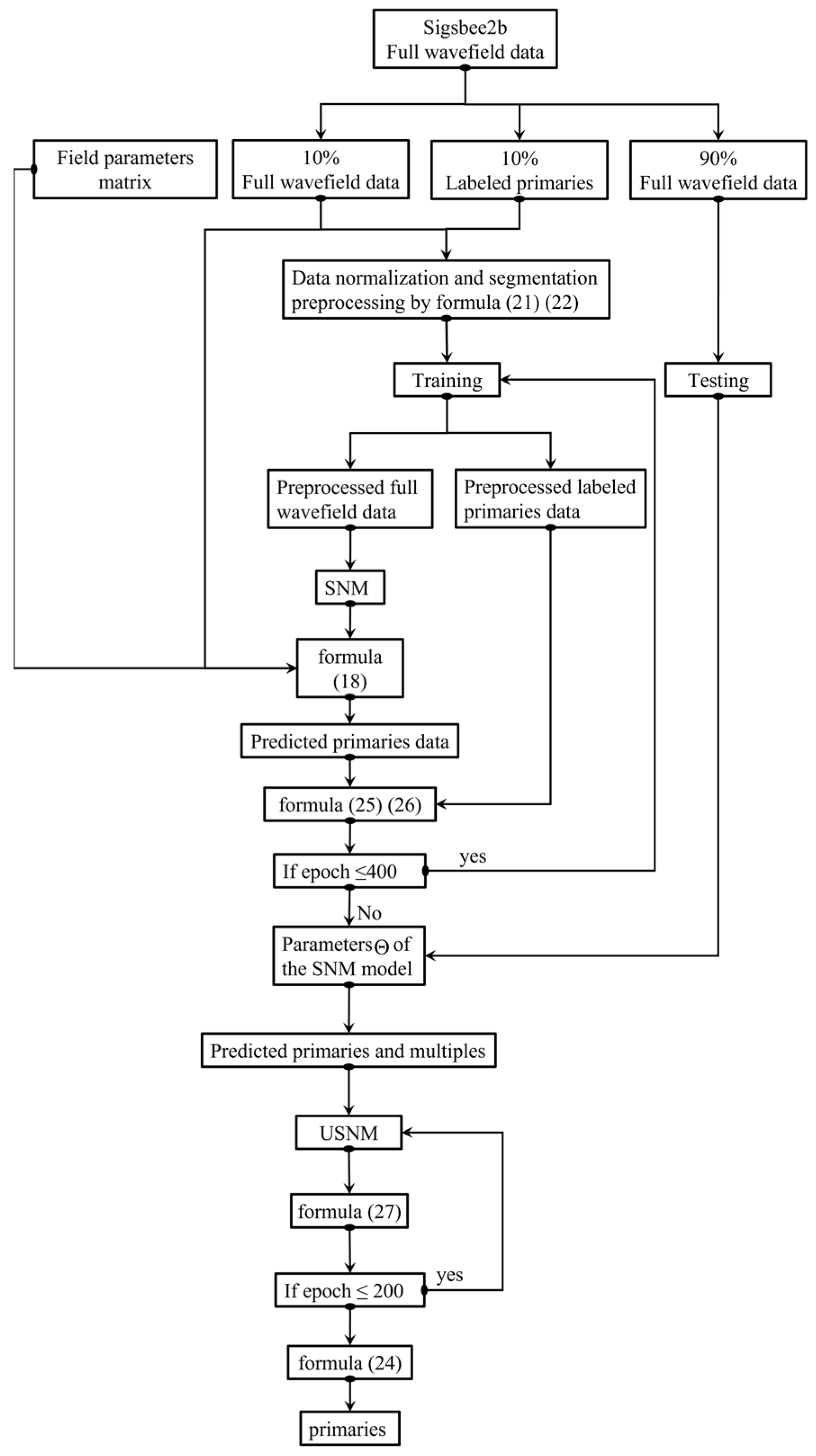
2. Methods
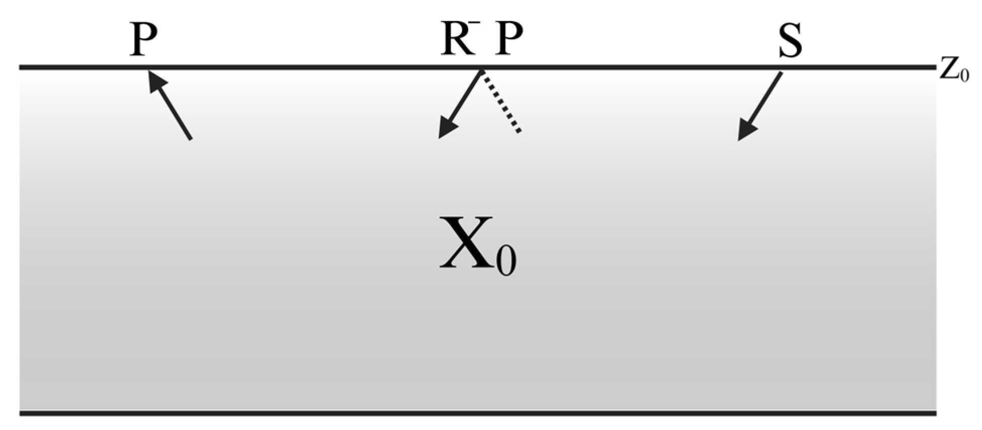
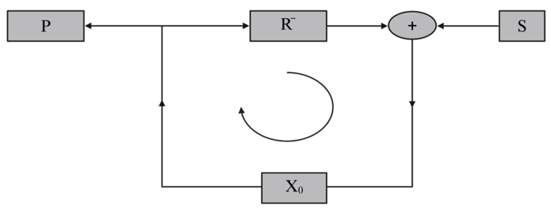
2.1. Surface-Related Multiple Elimination Method
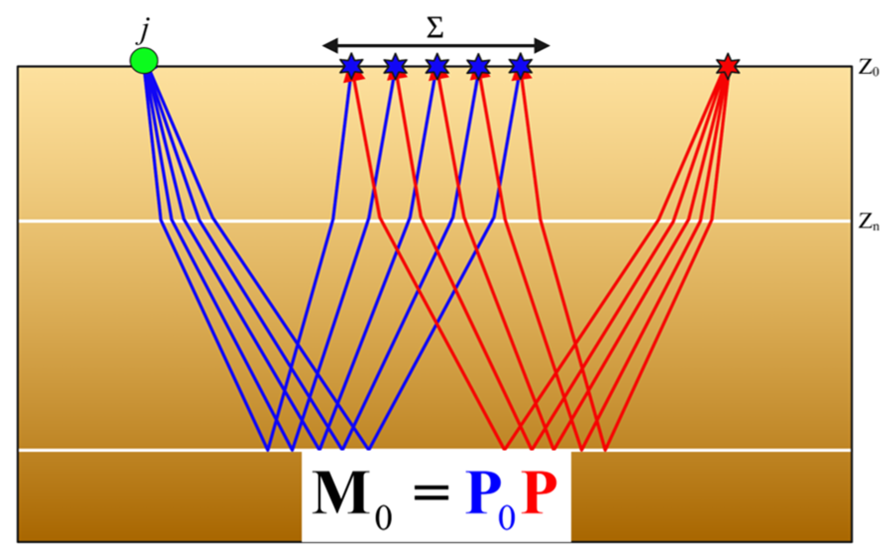
2.2. Polynomial Function Representation of the Primary
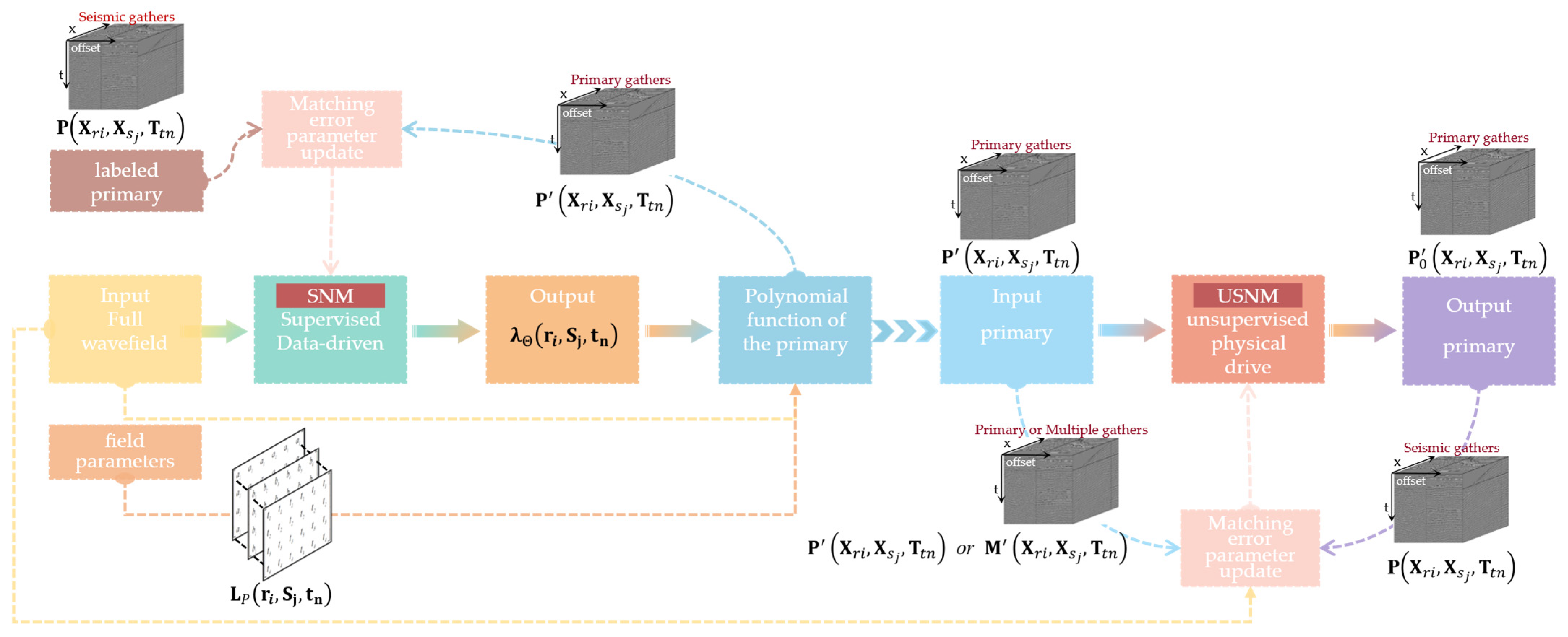
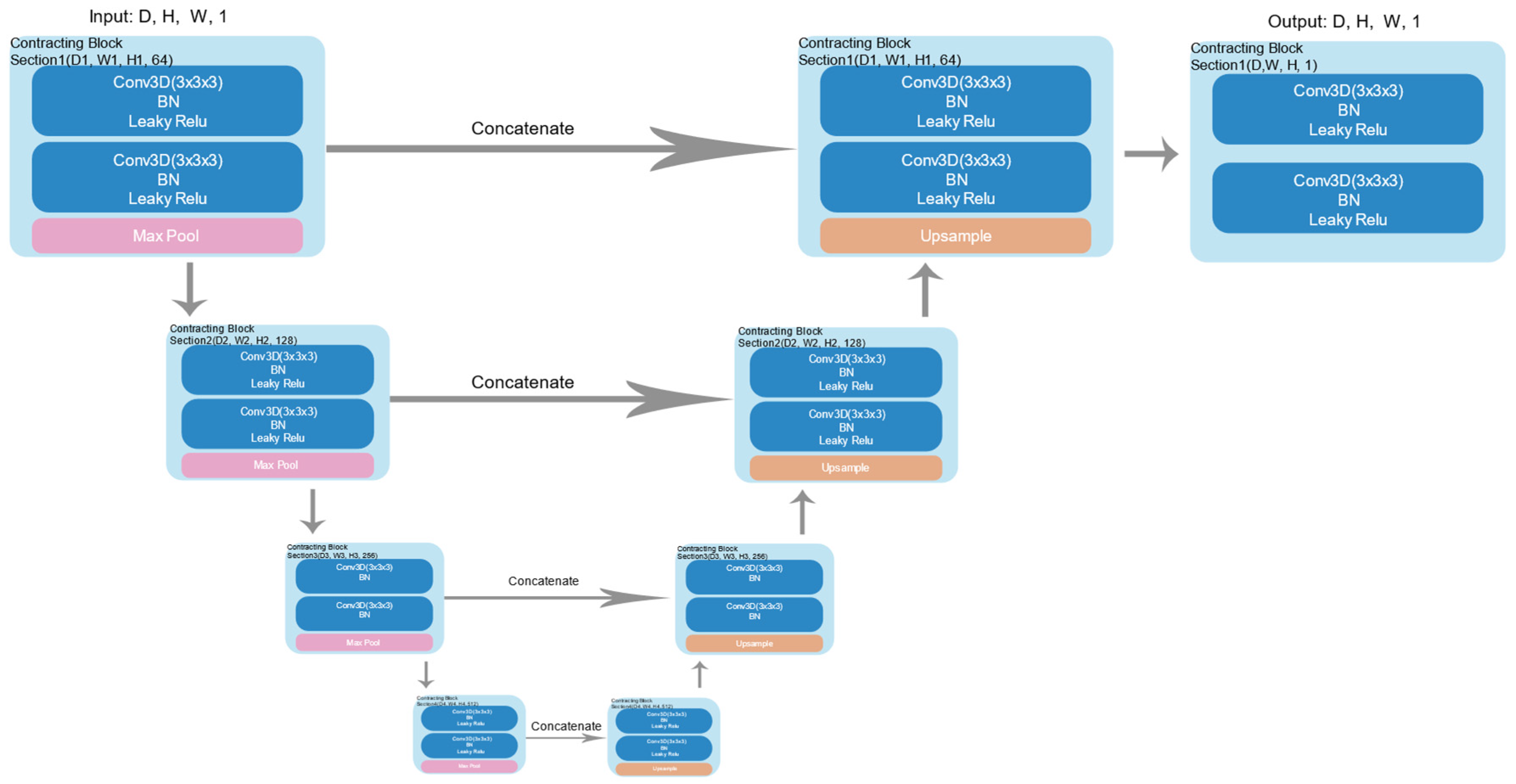
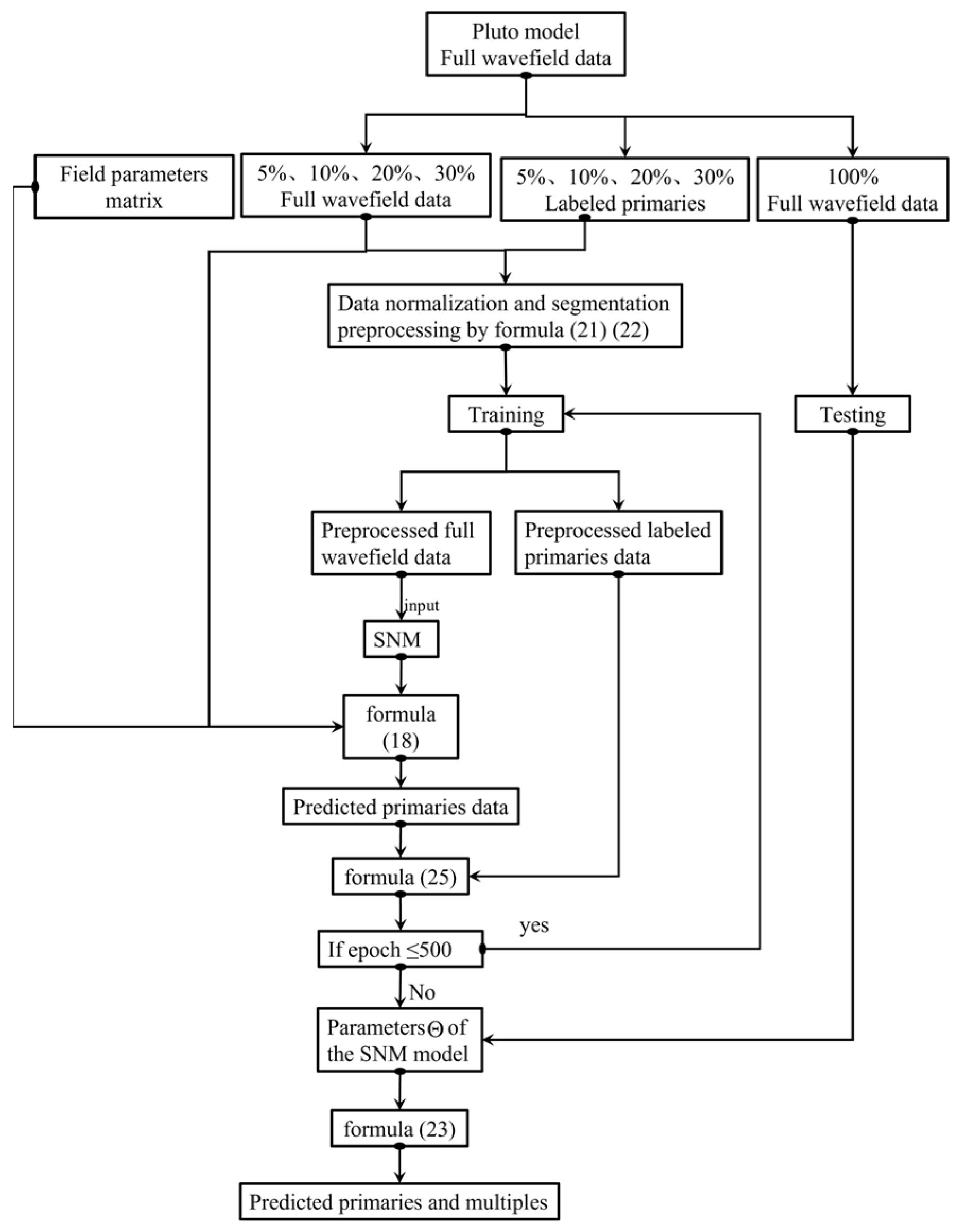
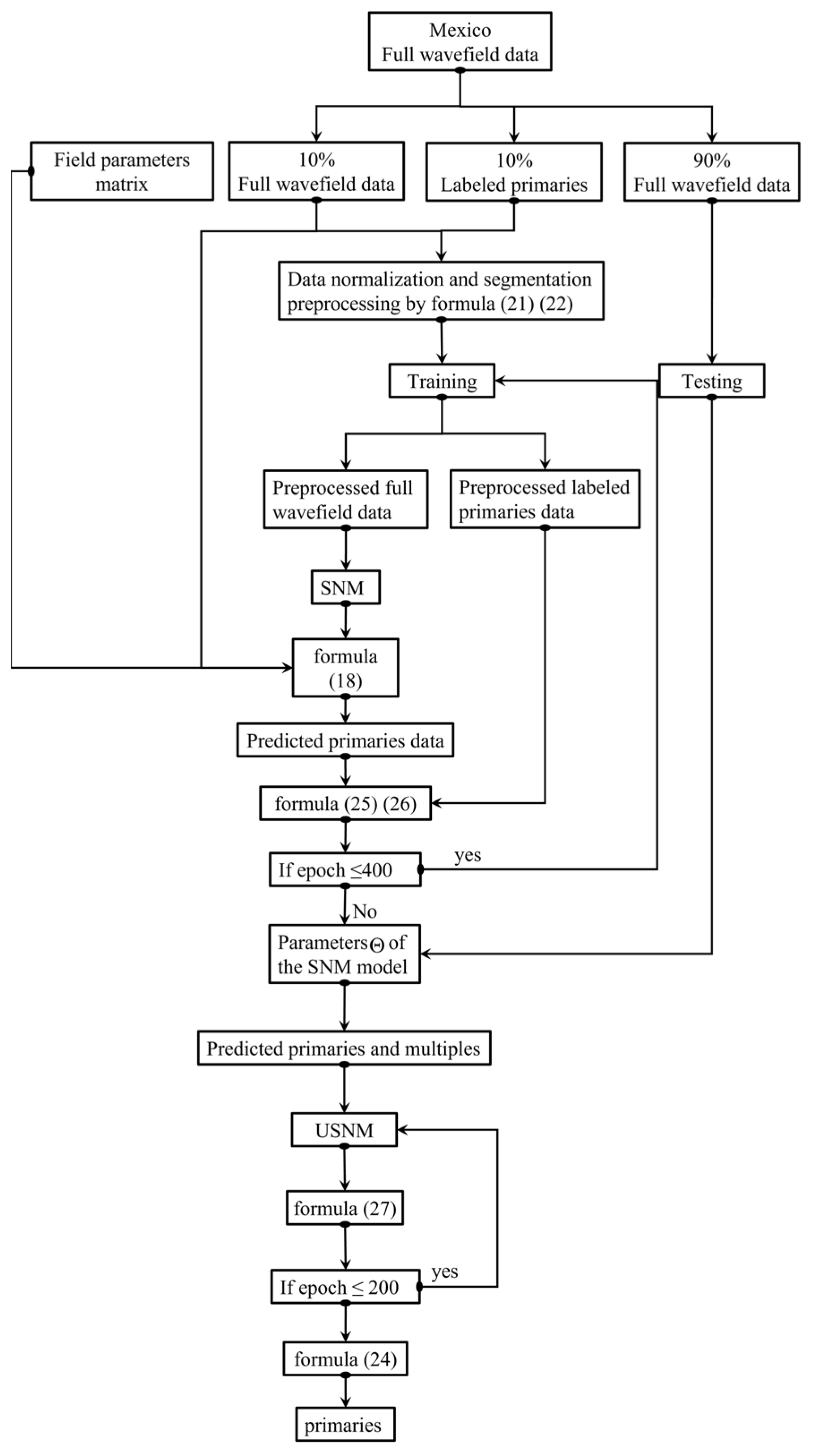
2.3. Field-Parameter-Guided Semi-Supervised Learning
2.4. Method for Evaluating the Model
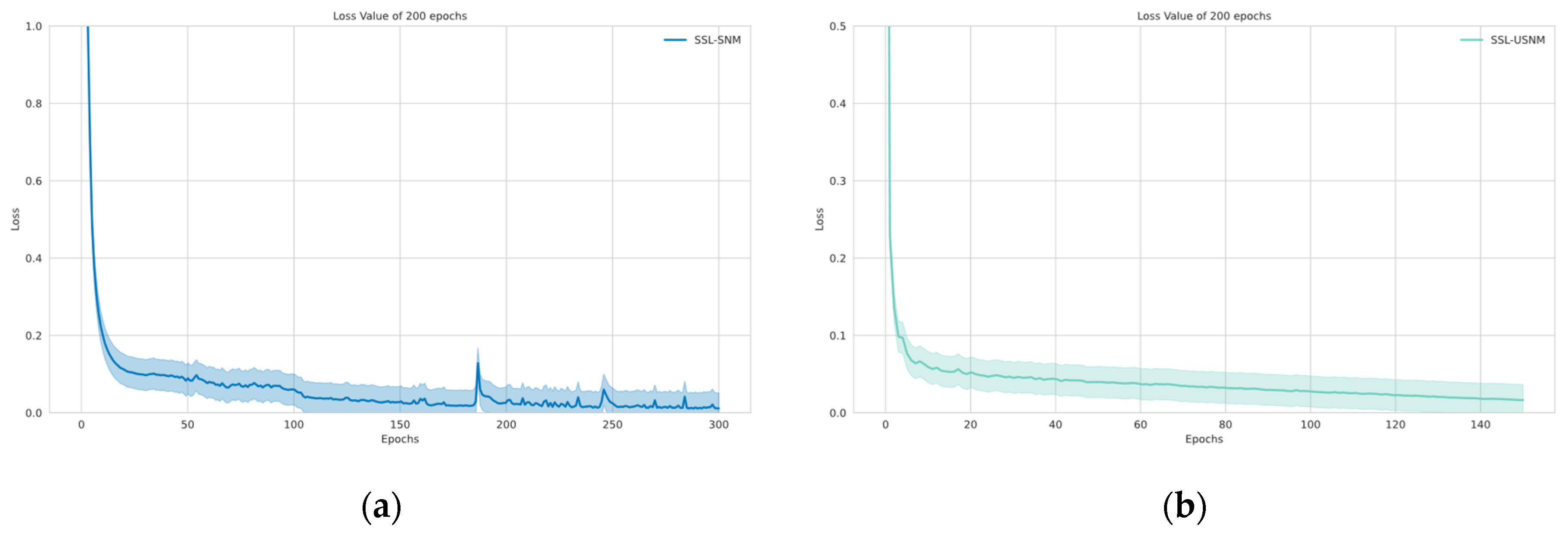
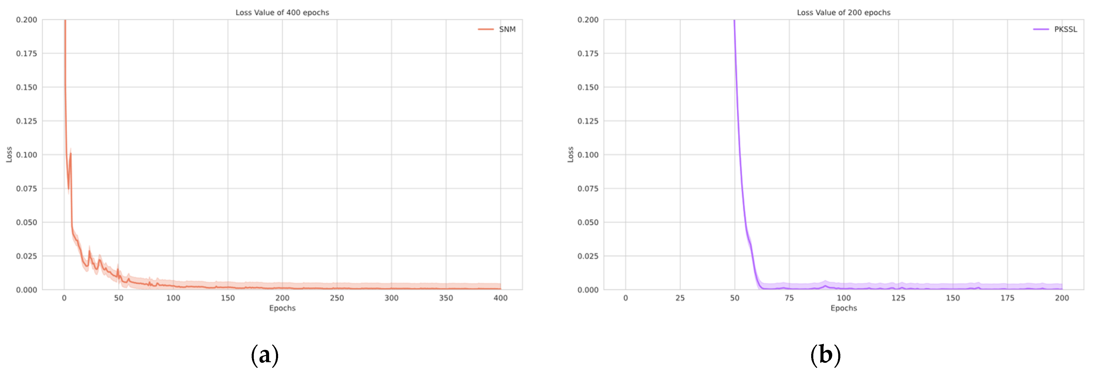
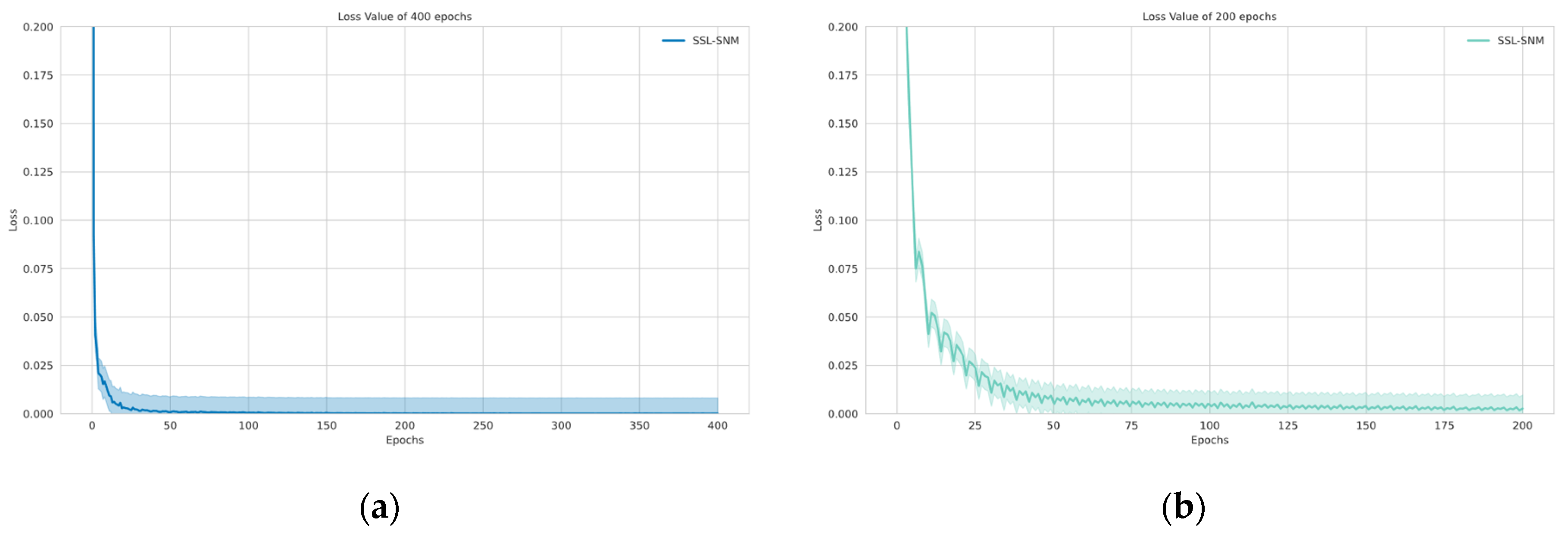
2.4.1. Loss Function for the FPSSL
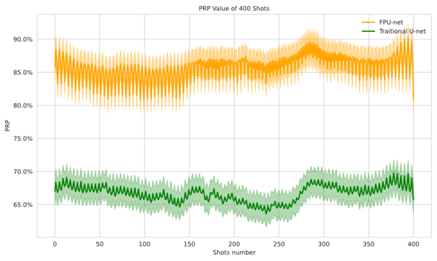
2.4.2. Primary Reconstruction Percentage
3. Results
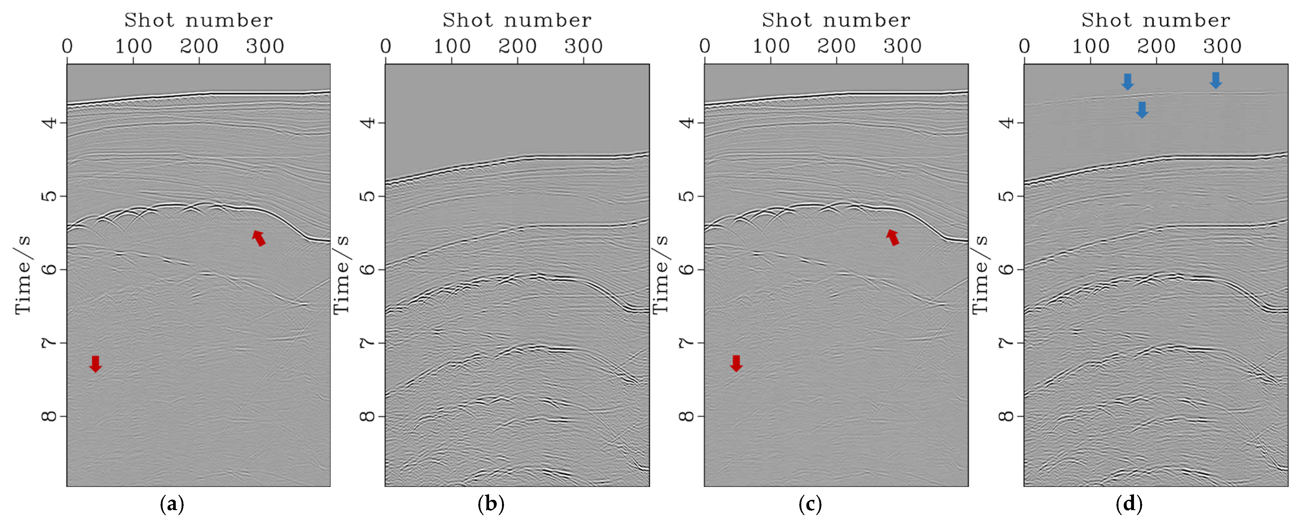
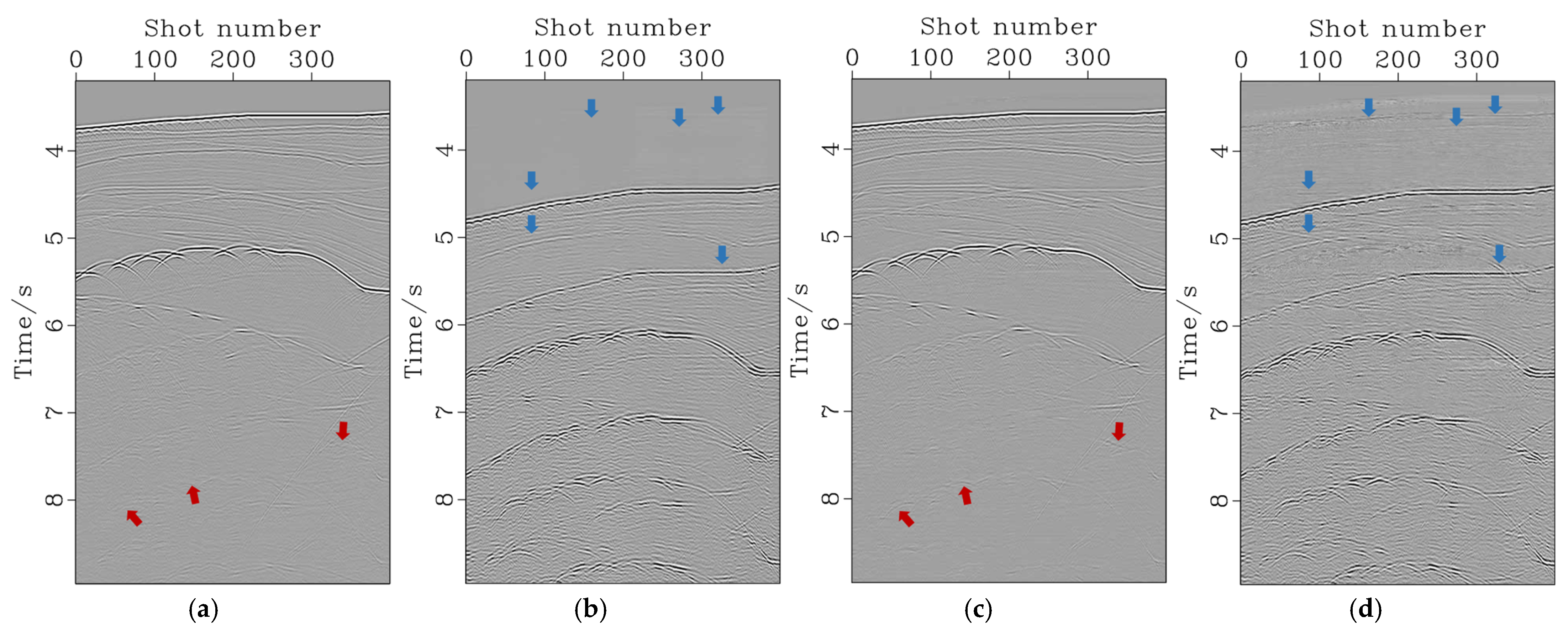
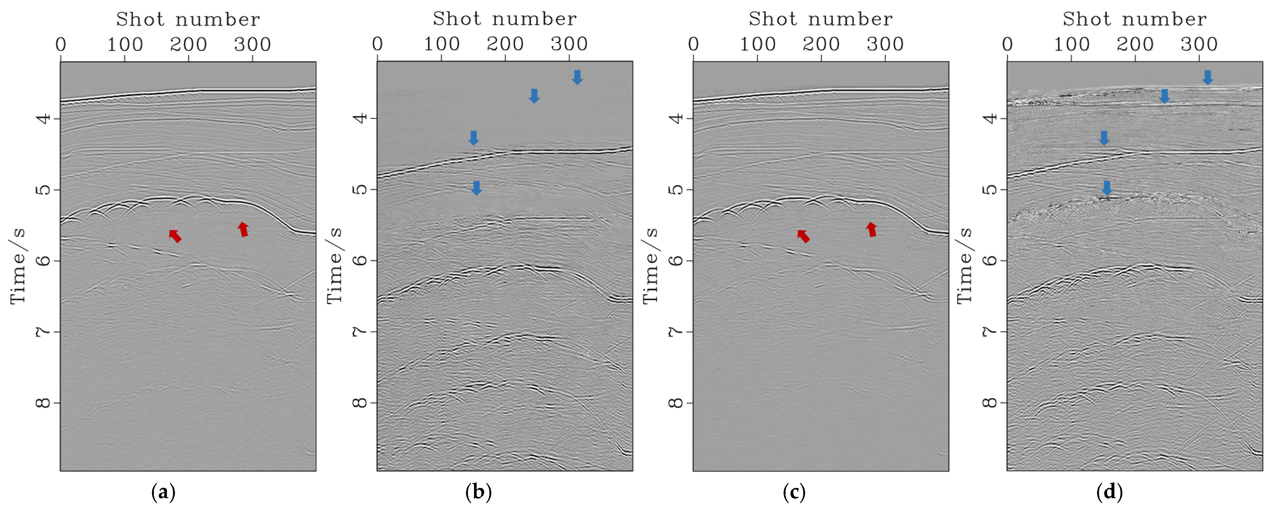
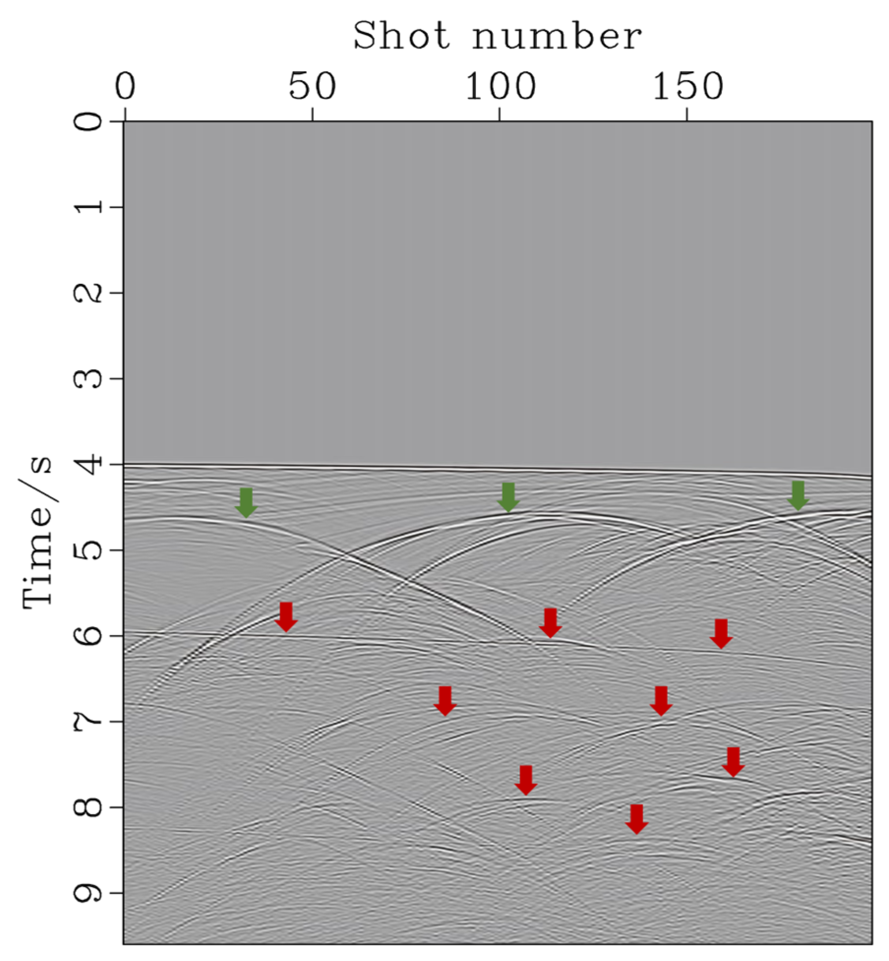
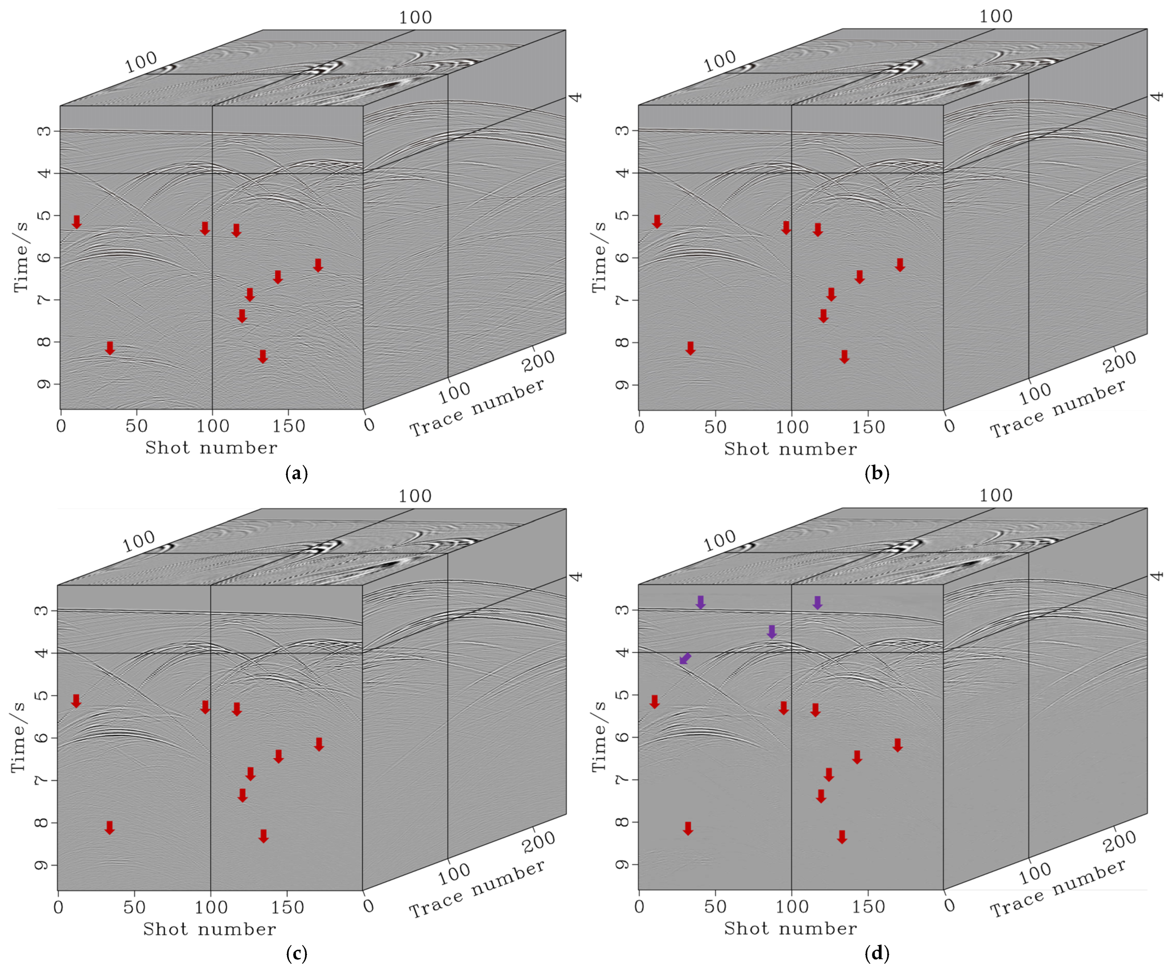
3.1. Pluto Data Result
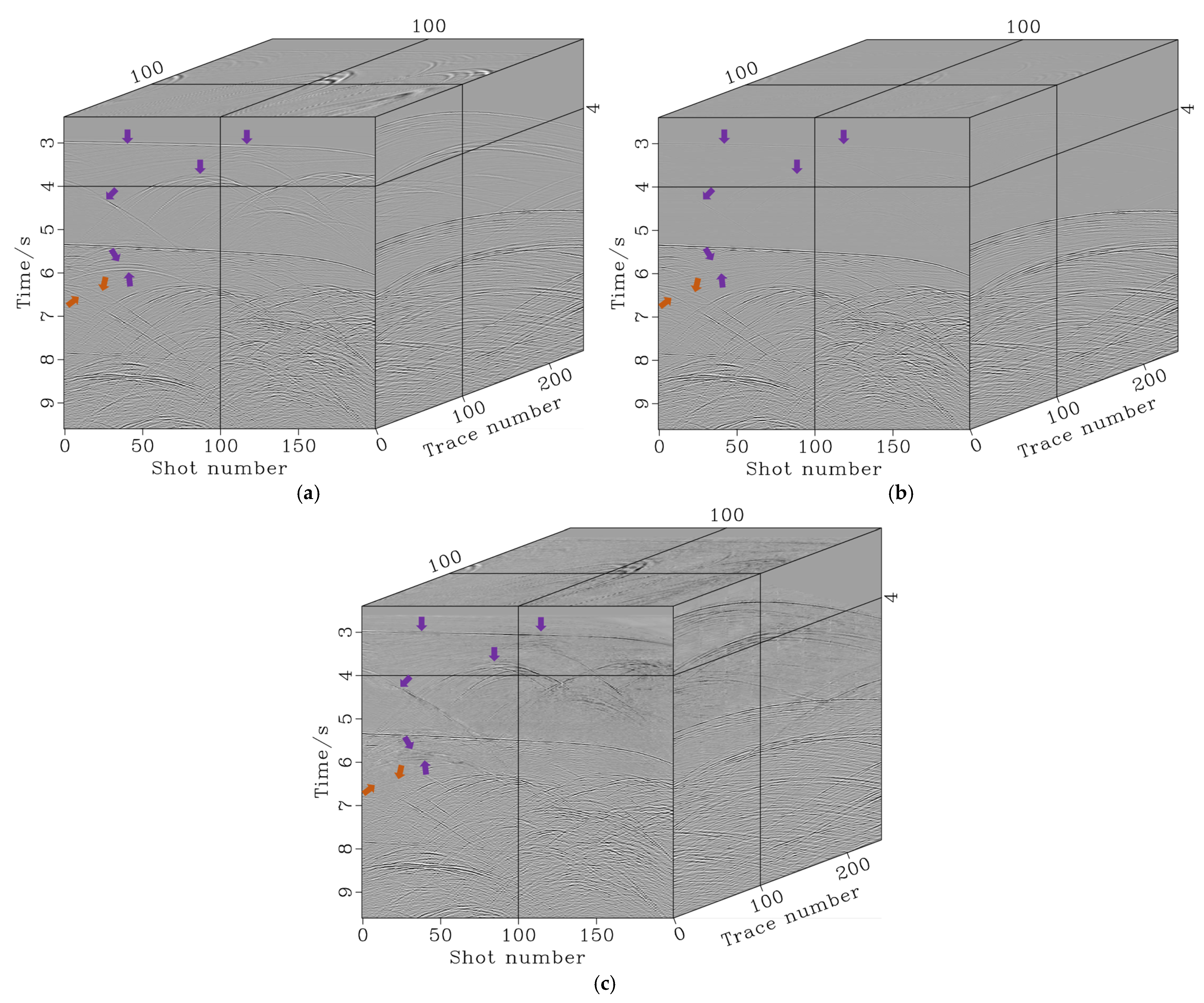
3.2. Sigsbee Data Result
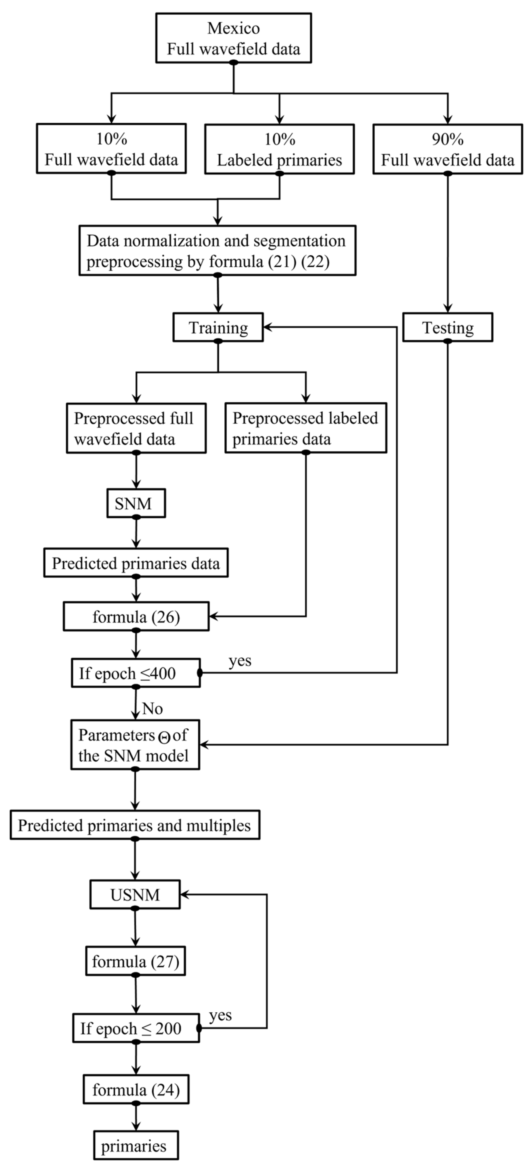
3.3. Real Marine Data Result
4. Conclusions
Author Contributions
Funding
Data Availability Statement
Conflicts of Interest
References
- Weglein, A.B. Multiple attenuation: An overview of recent advances and the road ahead (1999). Lead. Edge 1999, 18, 40–44. [Google Scholar] [CrossRef]
- Verschuur, D.J.; Berkhout, A.J. Seismic migration of blended shot records with surface-related multiple scattering. Geophysics 2011, 76, A7–A13. [Google Scholar] [CrossRef]
- Guitton, A.; Verschuur, D. Adaptive subtraction of multiples using the L1-norm. Geophys. Prospect. 2004, 52, 27–38. [Google Scholar] [CrossRef]
- Berkhout, J.; Verschuur, D.J. Estimation of multiple scattering by iterative inversion, Part I: Theoretical considerations. Geophysics 1997, 62, 1586–1595. [Google Scholar] [CrossRef]
- Shi, Y.; Jing, H.; Zhang, W.; Ning, D. Suppressing Multiples Using an Adaptive Multichannel Filter Based on L1-norm. Acta Geophys. 2017, 65, 667–681. [Google Scholar] [CrossRef]
- Li, Z. Adaptive multiple subtraction with a non-stationary regularization factor. J. Appl. Geophys. 2018, 159, 116–126. [Google Scholar] [CrossRef]
- Wang, Y. Multiple subtraction using an expanded multichannel matching filter. Geophysics 2003, 68, 346–354. [Google Scholar] [CrossRef]
- Saad, O.M.; Chen, Y. Deep denoising autoencoder for seismic random noise attenuation. Geophysics 2020, 85, V367–V376. [Google Scholar] [CrossRef]
- Liu, X.; Hu, T.; Wang, S.; Liu, T.; Wei, Z. Seismic Internal Multiple Suppression Based on Convolutional Neural Network. IEEE Geosci. Remote Sens. Lett. 2022, 19, 3008505. [Google Scholar] [CrossRef]
- Siahkoohi, A.; Verschuur, D.J.; Herrmann, F.J. Surface-related multiple elimination with deep learning. In Proceedings of the 89th Annual International Meeting, San Antonio, TX, USA, 15–20 September 2019; pp. 4629–4634. [Google Scholar] [CrossRef]
- Song, H.; Mao, W.; Tang, H. Appplication of deep neural networks for multiples attenuation. Chin. J. Geophys. 2021, 64, 2795–2808. [Google Scholar] [CrossRef]
- van Groenestijn, G.J.; Verschuur, D.J. Estimating primaries by sparse inversion and application to near- offset data reconstruction. Geophysics 2009, 74, A23–A28. [Google Scholar] [CrossRef]
- Tao, L.; Ren, H.; Ye, Y.; Jiang, J. Seismic Surface-Related Multiples Suppression Based on SAGAN. IEEE Geosci. Remote Sens. Lett. 2022, 19, 3006605. [Google Scholar] [CrossRef]
- Gu, Z.; Tao, L.; Ren, H.; Wu, R.; Geng, J. Internal multiple elimination with an inverse-scattering theory guided deep neural network. In Proceedings of the Second International Meeting for Applied Geoscience & Energy, Houston, TX, USA, 28 August–1 September 2022; pp. 2832–2836. [Google Scholar] [CrossRef]
- Wang, K.; Hu, T.; Wang, S.; Wei, J. Seismic multiple suppression based on a deep neural network method for marine data. Geophysics 2022, 87, V341–V365. [Google Scholar] [CrossRef]
- Durall, R.; Ghanim, A.; Ettrich, N.; Keuper, J. An in-depth study of U-net for seismic data conditioning: Multiple removal by moveout discrimination. Geophysics 2024, 89, WA233–WA246. [Google Scholar] [CrossRef]
- Qu, S.; Verschuur, E.; Zhang, D.; Cheng, Y. Training deep networks with only synthetic data: Deep-learning-based near-offset reconstruction for (closed-loop) surface-related multiple estimation on shallow-water field data. Geophysics 2021, 86, A39–A43. [Google Scholar] [CrossRef]
- Liu, L.; Hu, T.; Huang, J.; Wang, S. Adaptive Surface-Related Multiple Subtraction Based on Convolutional Neural Network. IEEE Geosci. Remote Sens. Lett. 2022, 19, 8021905. [Google Scholar] [CrossRef]
- Zhang, D.; de Leeuw, M.; Verschuur, E. Deep learning-based seismic surface-related multiple adaptive subtraction with synthetic primary labels. In Proceedings of the First International Meeting for Applied Geoscience & Energy, Denver, CO, USA, 26 September–1 October 2021; pp. 2844–2848. [Google Scholar] [CrossRef]
- Lang, X.; Li, C.; Wang, M.; Li, X. Semi-Supervised Seismic Impedance Inversion With Convolutional Neural Network and Lightweight Transformer. IEEE Trans. Geosci. Remote Sens. 2024, 62, 4506511. [Google Scholar] [CrossRef]
- Ge, M.; Zheng, W.; Wang, W. Semi-supervised impedance inversion by Bayesian neural network based on 2-d CNN pre-training. In Proceedings of the SEG 2021 Workshop: 4th International Workshop on Mathematical Geophysics: Traditional & Learning, Virtual, 17–19 December 2021; pp. 129–133. [Google Scholar] [CrossRef]
- Alfarraj, M.; AIRegib, G. Semi-supervised learning for acoustic impedance inversion. In Proceedings of the SEG International Exposition and Annual Meeting, San Antonio, TX, USA, 15–20 September 2019; pp. 2298–2302. [Google Scholar] [CrossRef]
- Xu, Z.; Li, K.; Huang, Z.; Yin, R.; Fan, Y. 3-D Salt Body Segmentation Method Based on Multiview Co-Regularization. IEEE Trans. Geosci. Remote Sens. 2024, 62, 5913013. [Google Scholar] [CrossRef]
- Wang, Z.; Wang, S.; Zhou, C.; Cheng, W. AVO Inversion Based on Closed-Loop Multitask Conditional Wasserstein Generative Adversarial Network. IEEE Trans. Geosci. Remote Sens. 2023, 61, 5906013. [Google Scholar] [CrossRef]
- Wang, K.; Hu, T.; Wang, S. Surface-related multiple attenuation based on a self-supervised deep neural network with local wavefield characteristics. Geophysics 2023, 88, V387–V402. [Google Scholar] [CrossRef]
- Wang, K.; Hu, T.; Wang, S. Unsupervised Learning for Seismic Internal Multiple Suppression Based on Adaptive Virtual Events. Geophysics 2022, 60, 5914013. [Google Scholar] [CrossRef]
- Qi, G.; Luo, J. Small Data Challenges in Big Data Era: A Survey of Recent Progress on Unsupervised and Semi-Supervised Methods. IEEE Trans. Pattern Anal. Mach. Intell. 2022, 44, 2168–2187. [Google Scholar] [CrossRef]
- Li, Y.; Chen, J.; Xie, X.; Ma, K.; Zheng, Y. Self-Loop Uncertainty: A Novel Pseudo-Label for Semi-Supervised Medical Image Segmentation. arXiv 2020, arXiv:2007.09854. [Google Scholar] [CrossRef]
- Ouali, Y.; Hudelot, C.; Tami, M. An Overview of Deep Semi-Supervised Learning. arXiv 2020, arXiv:2006.05278. [Google Scholar] [CrossRef]
- Wu, X.; Ma, J.; Si, X.; Bi, Z.; Yang, J.; Gao, H.; Xie, D.; Guo, Z.; Zhang, J. Sensing Prior Constraints in Deep Neural Networks for Solving Exploration Geophysical Problems. Proc. Natl. Acad. Sci. USA 2023, 120, e2219573120. [Google Scholar] [CrossRef]
- Ronneberger, O.; Fischer, P.; Brox, T. U-Net: Convolutional Networks for Biomedical Image Segmentation. In Proceedings of the 18th Conference on Medical Image Computing and Computer-Assisted Intervention, Munich, Germany, 5–9 October 2015; pp. 234–241. [Google Scholar]
- Wu, X.; Shen, C. A new methodology for local cross-correlation between two nonstationary time series. Phys. A Stat. Mech. Its Appl. 2019, 528, 121307. [Google Scholar] [CrossRef]
- Waheed, U.; Haghighat, E.; Alkhalifah, T.; Song, C.; Hao, Q. PINNeik: Eikonal solution using physics-informed neural networks. Comput. Geosci. 2021, 155, 104833. [Google Scholar] [CrossRef]
- Mishra, S.; Molinaro, R. Estimates on the generalization error of physics-informed neural networks for approximating a class of inverse problems for PDEs. IMA J. Numer. Anal. 2022, 42, 981–1022. [Google Scholar] [CrossRef]
- Brinker, A. Calculation of the local cross-correlation function on the basis of the Laguerre transform. IEEE Trans. Signal Process. 1993, 41, 1980–1982. [Google Scholar] [CrossRef]
- Zhang, T.; Ma, X.; Zhan, Z.; Zhou, S.; Ding, C.; Fardad, M.; Wang, Y. A unified DNN weight pruning framework using reweighted optimization methods. In Proceedings of the 58th ACM/IEEE Design Automation Conference, San Francisco, CA, USA, 5–9 December 2021; pp. 493–498. [Google Scholar]
- Liu, J.; Hu, T.; Peng, G.; Cui, Y. Removal of internal multiples by iterative construction of virtual primaries. Geophys. J. Int. 2018, 215, 81–101. [Google Scholar] [CrossRef]


| Different Percentage | 30% | 20% | 10% | 5% | |
|---|---|---|---|---|---|
| PRP Value | |||||
| FPU-net | 95.2% | 91.8% | 84.3% | 78.04% | |
| Traditional U-net | 80.8% | 77.2% | 68.1% | 63.3% | |
| Difference in PRP value in FPU-net and TU-net | 14.4% | 14.6% | 16.2% | 14.73% | |
| Average PRP difference value | 15% | ||||
Disclaimer/Publisher’s Note: The statements, opinions and data contained in all publications are solely those of the individual author(s) and contributor(s) and not of MDPI and/or the editor(s). MDPI and/or the editor(s) disclaim responsibility for any injury to people or property resulting from any ideas, methods, instructions or products referred to in the content. |
© 2025 by the authors. Licensee MDPI, Basel, Switzerland. This article is an open access article distributed under the terms and conditions of the Creative Commons Attribution (CC BY) license (https://creativecommons.org/licenses/by/4.0/).
Share and Cite
Qi, J.; Cao, S.; Wang, Z.; Xu, Y.; Zhang, Q. Surface-Related Multiple Suppression Based on Field-Parameter-Guided Semi-Supervised Learning for Marine Data. J. Mar. Sci. Eng. 2025, 13, 862. https://doi.org/10.3390/jmse13050862
Qi J, Cao S, Wang Z, Xu Y, Zhang Q. Surface-Related Multiple Suppression Based on Field-Parameter-Guided Semi-Supervised Learning for Marine Data. Journal of Marine Science and Engineering. 2025; 13(5):862. https://doi.org/10.3390/jmse13050862
Chicago/Turabian StyleQi, Jiao, Siyuan Cao, Zhiyong Wang, Yankai Xu, and Qiqi Zhang. 2025. "Surface-Related Multiple Suppression Based on Field-Parameter-Guided Semi-Supervised Learning for Marine Data" Journal of Marine Science and Engineering 13, no. 5: 862. https://doi.org/10.3390/jmse13050862
APA StyleQi, J., Cao, S., Wang, Z., Xu, Y., & Zhang, Q. (2025). Surface-Related Multiple Suppression Based on Field-Parameter-Guided Semi-Supervised Learning for Marine Data. Journal of Marine Science and Engineering, 13(5), 862. https://doi.org/10.3390/jmse13050862