Article

Analysis of the Accuracy of a Body-Force Propeller Model and a Discretized Propeller Model in RANS Simulations of the Flow Around a Maneuvering Ship

by
Long Jiang
1,*,
Jianxi Yao
1,2 and
Zuyuan Liu
1,2
1
School of Naval Architecture, Ocean and Energy Power Engineering, Wuhan University of Technology, Wuhan 430062, China
2
Key Laboratory of High-Performance Ship Technology (Wuhan University of Technology), Ministry of Education, Wuhan 430062, China
*
Author to whom correspondence should be addressed.
J. Mar. Sci. Eng. 2025, 13(4), 788; https://doi.org/10.3390/jmse13040788
Submission received: 12 March 2025 / Revised: 8 April 2025 / Accepted: 14 April 2025 / Published: 15 April 2025
(This article belongs to the Section Ocean Engineering)

Abstract

:
Currently, the RANS (Reynolds-Averaged Navier–Stokes) method is widely recognized as a prevalent approach for computing ship maneuvering forces and moments. Obtaining hydrodynamic derivatives using pure RANS is time-consuming, especially with rotating propellers. A reasonable simplification of the propeller is usually necessary to improve simulation efficiency. The ITTC suggests both the discretized propeller model (DPM) and the body-force model (BFM) for RANS simulations. While BFM offers computational efficiency, it may not accurately represent large-amplitude ship maneuvers. It is quite significant to figure out how BFM affects numerical accuracy. This study compares the DPM and a very simple BFM in RANS simulations of the KCS (KRISO Container Ship), focusing on static rudder, drift, and circle motion tests. The main purpose is to check the differences between the simulated results by using the BFM and DPM. While side forces and yaw moments from both models are similar, discrepancies in longitudinal forces increase with higher rudder angles, drift angles, or turning rates. Errors in side forces and yaw moments are under 10% for both models, compared with experimental data. But BFM’s longitudinal force errors exceed 20% at large motion amplitudes, indicating reduced accuracy compared to DPM. The results of the BFM method are subject to two main sources of error. First, the lack of physical shape representation for the propeller blades leads to the absence of lather force during rotation. This in turn results in an inaccurate prediction of the interaction between the propeller blade root or blade tip leakage vortices and the rudder. Second, the limitations of the adopted model prevent it from accurately providing the thrust and torque generated by the propeller under actual operating conditions.

1. Introduction

Predicting ship maneuverability is crucial for ensuring navigation safety, and the IMO [1] (International Maritime Organization) mandates its assessment during the initial ship design phase. There are usually two ways to predict ship maneuverability in the early stages of ship design. One is to conduct a free-running model test to evaluate the maneuverability of the ship through direct indicators, such as the tactical diameter and first overshoot angle; the other is to employ a system-based method, in which the ship motion equations are solved by using hydrodynamic models with corresponding hydrodynamic derivatives. The captive model test is usually used to obtain the hydrodynamic derivatives.
These maneuverability assessments, which include free-running and captive model tests, are typically carried out through physical modeling or CFD simulations. Free-running model tests have always been highly valued and widely conducted by ship maneuverability researchers [2]. Similarly, as the most reliable method for obtaining hydrodynamic derivatives, captive model tests in physical towing tanks have also made significant progress. Some well-known tanks, such as FORCE, IIHR (Iowa Institute of Hydraulic Research), and CSSRC (China Ship Scientific Research Centre), have conducted a series of captive model tests on different ship types [3,4,5]. In addition, Yun et al. [6] conducted free-running model tests on the KRISO Container Ship (KCS), examining various conditions such as the trimmed state, heeled state, and scenarios with a reduced metacentric height (GM). The outcomes of these tests serve as benchmark datasets for subsequent simulation studies. Yeo et al. [7] performed captive model tests on the KCS to investigate the impact of heel angles. They conducted a series of maneuvering simulations utilizing hydrodynamic derivatives obtained from the model tests. The findings indicated variations in turning and zigzag behaviors corresponding to different heel angles. Yeo et al. [7] performed captive model tests on the KCS to investigate the impact of heel angles. They conducted a series of maneuvering simulations utilizing hydrodynamic derivatives obtained from the model tests. The findings indicated variations in turning and zigzag behaviors corresponding to different heel angles.
In the past two decades, with the rapid development of computer science and CFD-based numerical tank technology, simulations of ship maneuvering experiments conducted in virtual tanks have become increasingly popular due to their low cost and ability to obtain detailed flow field information [8]. A series of studies conducted by IIHR indicate that virtual experiments have the potential to replace real model experiments for ship maneuvering prediction [9,10,11].
Following Prandtl’s introduction of the mixed-length model in 1925 [12], numerous Reynolds stress closure models have been developed within the RANS (Reynolds-Averaged Navier–Stokes) framework, which have been extensively utilized for simulating both free-running and captive model tests. In the realm of free-running model tests, Jin et al. [13] employed the URANS (Unsteady Reynolds-Averaged Navier–Stokes) solver to simulate the self-propelled turning circle and zigzag maneuvers of the benchmark combatant DTMB 5415M. Additionally, Wang J. et al. [14] employed their proprietary CFD solver, naoe-FOAM-SJTU, to simulate the zigzag maneuvers of a fully rigged ONRT model under both calm water and wave conditions. They utilized dynamic overset grid technology to handle complex ship motions involving propellers and rudders and OpenFOAM’s waves2Foam library for wave generation.
In terms of captive model tests, Cura-Hochbaum [15] outlined a methodology for forecasting a ship’s maneuvering characteristics by virtually conducting PMM tests to ascertain the maneuvering derivatives. This approach simulates the flow around a twin-screw ship model executing motions akin to those in captive model tests, utilizing a RANS code founded on finite volume techniques. Turbulence is modeled using a two-equation k-ω model, and a body-force model is employed to approximate the propeller’s impact on the flow. Duman and Bal [16] utilized an unsteady RANS solver based on the finite volume method (FVM) to forecast the maneuvering coefficients of a catamaran, highlighting the feasibility of CFD in predicting such coefficients. Visonneau et al. [17] also relied on the FVM-based approach to analyze the flow around a surface combatant under diverse static drift and dynamic sway scenarios. In the realm of open-source software, Islam and Guedes Soares [18] harnessed OpenFOAM to derive hydrodynamic derivatives, demonstrating its utility in maneuverability studies. Silva and Aram [19] turned to NavyFOAM, an in-house CFD solver, for captive model simulations of the ONRT, examining its behavior under various conditions. Sukas et al. [20] adopted a system-based strategy to anticipate the maneuvering performance of a twin-propeller/twin-rudder ship, integrating URANS-derived hydrodynamic derivatives into an MMG model for simulating turning circle and zigzag maneuvers. Sakamoto et al. [21] paralleled this approach, employing a CFD-MMG method to forecast ship maneuvering, underscoring the synergy between CFD and maneuvering modeling.
The ultimate goal of CFD simulations is to predict the hydrodynamic performance and maneuvering behaviors of full-scale ships with actual attachments (such as rudders, propellers, and bilge keels) under actual conditions [11,22]. However, as Stern et al. [23] pointed out, due to the complexity of the problem, limitations of numerical techniques, and high-performance calculations, this remains a huge challenge. And reasonable assumptions or simplifications are often considered to reduce the computational time for given practical problems. Currently, for maneuverability researchers, the balance between the economy and accuracy of maneuverability prediction is a key focus.
The numerical modeling of propellers in CFD simulations is a key issue in accurately predicting the interaction between hull propellers and rudders, rudder control characteristics, and the flow field in the stern region. There are two numerical propeller models recommended by the ITTC in the RANS method, including the discretized propeller model (DPM) and the body-force model (BFM). Pankajakshan et al. [24] conducted virtual free self-propelled maneuverability tests using rotating propellers and rotatable rudders. They calculated the horizontal motion of a submarine body using the code UNCLE. The rotation of the propeller was achieved by sliding grids, and the deflection of the rudder was achieved by multi-grid interpolation. The computed results are in good agreement with the experimental data. However, compared to the simulations with BFM, considering discrete propellers in numerical simulation is very time-consuming. For example, in the study by Carrica et al. [11], the number of grids was as high as 71.3 million, with a time step as small as milliseconds. The simulation time for a direct free-running maneuverability test condition was as long as 20 days. In addition, although the discrete propeller was used in the research of Carrica et al. [9], it was stated at the end of the article that their future efforts will be to use the BFM to approximate the rotational effect of propellers on the flow field in order to reduce computational costs.
BFM seems to show its reliability and computational efficiency within a certain range. In the research of Cura-Hochbaum [25], a body-force model is used to approximate the propeller effects on the flow. Carrica et al. [26] studied the broaching event of ONRT with appendages such as rudders and bilge keels in irregular waves using a propeller of the BFM based on CFDShip-Iova v4.0.
The distribution of the BFM depends on the actual velocity field, which in turn depends on the rotation of the blades. Therefore, a practical model should have considered the interaction between the actual velocity field and the rotation of the propeller blades, and an iterative process should be required to determine the stable flow field due to the nonlinearity of this interaction. However, the Hougha–Ordway models [27] in the aforementioned literature [10,11,25,28] often overlook the special physical phenomena that occur when propellers operate under maneuvering conditions. Based on this, some scholars have compared the prediction results of the two propulsion methods in free-running simulations. Jin et al. [13] utilized their URANS solver to simulate the turning circle and zigzag maneuvers of the DTMB 5415M model, employing both the DPM and BFM for propulsion under calm water and wave conditions. Yu et al. [2] focused on the DPM and evaluated three distinct BFMs for ship turning circle simulations, enhancing the understanding of maneuvering dynamics.
While existing research comparing the body-force model (BFM) and discrete propeller model (DPM) has primarily focused on straight-ahead sailing conditions [29], some studies on maneuverability either do not involve rudder deflection [30] or fail to illustrate the rudder angle’s impact on the propeller. Additionally, comparisons from free-running experiments [31,32] do not provide a detailed analysis of the variations in the propeller wake field under different maneuvering conditions, such as varying drift angles, rudder angles, and yaw rates. Compared to free-running model tests, captive model tests are more favorable for investigating the physical mechanisms that influence maneuverability. Therefore, this study explores the effect of different propeller models on the precision of computed forces and moments experienced by a ship during captive model tests. RANS simulations of a KCS in static drift and moving in circular motions are carried out in this work. Two different propulsion technologies, the BFM and DPM, are adopted. To study the impact of ship speed on the simulation results, three ship speeds are considered, corresponding to Froude numbers F r = 0.156, 0.201, and 0.260. Firstly, verification and validation studies are conducted on numerical uncertainty. Secondly, the computed results obtained by using the two propulsion models are compared with each other and with experimental data. Finally, the reasons for the differences in the results are analyzed based on the force curve and flow field diagrams. The results indicate that compared to BFM, DPM has advantages in providing more accurate predictions of ship maneuvering forces and moments. Generally speaking, the difference between experimental data and numerical results of BFM is mostly below 10%. Especially for the simulation results with a small drift angle and small rudder angle, the predictions are highly accurate. Additionally, the discussion also covered the error sources of the BFM. One of which is the lack of physical shape, and another is that the adopted BFM cannot accurately provide thrust and torque under actual maneuvering conditions.

2. Numerical Methodology

2.1. Governing Equations

A right-hand ship-fixed coordinate system is employed to depict the fluid dynamics surrounding the ship. The origin o is positioned where the mid-ship section, the center-line plane, and the still water plane intersect. The x -axis directs towards the bow, the y -axis towards the starboard, and the z -axis towards the keel. For incompressible Newtonian fluids, the continuity equation (mass conservation) and RANS equations (momentum conservation) are formulated as
U i x i = 0
U i t + U j U i x j = f i 1 ρ p x i + x j ν U i x j + U j x i U i U j ¯ u i t + ε i j k Ω j u k ε i j k ω j ε k m n Ω m x n 2 ε i j k Ω j U k ε i j k Ω j t x k
In these equations, the subscripts i, j, and k take values from 1 to 3. U i = ( U , V , W ) and x i = ( x , y , z ) represent the flow velocity and independent Cartesian coordinates, respectively. u i = ( u , v , w ) represents the independent Cartesian coordinates. Ω i = ( p , q , r ) represents the ship’s linear and angular velocities, f i denotes the body-force source term per unit mass, ν is the kinematic viscosity, and ε i j k is the permutation symbol.
When compared to the RANS equations in the Earth’s fixed inertial reference frame, there are four additional terms on the right of the RANS equations. These terms are, in order, the unit mass translational acceleration, the unit mass centrifugal force, the unit mass Coriolis force, and the unit mass angular acceleration. In our previous work, these inertia terms have been programmed into OpenFOAM-v1612+ [33].
The term ρ U i U j ¯ in Equation (2) refers to Reynolds stress. Based on the Boussinesq assumption, the specific Reynolds stress is expressed as
U i U j ¯ = ν t ( U i ¯ x j + U j ¯ x i ) 2 3 k δ i j
where ν t is the eddy viscosity, k is the turbulent kinetic energy, and δ i j is the Kronecker symbol.
To close the RANS equations, the k-ω SST model with wall functions [34] is used to close the RANS equations in this study. And the coefficients in the model are listed in Table 1.

2.2. VOF Equations

In this article, all of the simulations utilize water–air flow. The VOF (Volume of Fluid) method is employed to describe the free surface. The corresponding transport equation is
α t + ( α U i ) x i = 0
where the fraction function α represents that a computational cell with α = 0 is full of air, if α = 1 it is full of water, and if 0 < α < 1 the cell locates at the interface between water and air. The fluid density and viscosity were computed by Hirt and Nichols (1981) [35]:
ρ = ρ w a t e r α + ρ a i r 1 α
ν = ν w a t e r α + ν a i r 1 α
The interFoam solver, a classical algebraic VOF solver in OpenFOAM, was employed for simulating free-surface flows. It relies on the concept of limiters, where first-order and higher-order schemes are combined to maintain the sharpness and boundedness of the VOF field.

2.3. Body-Force Propeller Model

In the simulations based on BFM, a basic body-force model (H-O model) is employed to approximate the impact of a real rotating propeller. Within the body-force region, the term f i in the RANS equations is not zero. The axial and tangential body-force distributions on the propeller disk follow previous studies like Stern et al. [36]
f b x = A x R * 1 R *
f b θ = A θ R * 1 R * R * ( 1 R h ) + R h
where
R * = R R h 1 R h
R = R R P
R h = R H R P
A x = 105 8 T π δ P ( 3 R H + 4 R P ) ( R P R H )
A θ = 105 8 Q π δ P R P ( 3 R H + 4 R P ) ( R P R H )
The body-force propeller is confined within a cylinder defined by π ( R P 2 R H 2 ) δ P , where R P is the propeller radius, R H is the hub radius, δ P is the thickness, and R is the virtual propeller disk radius. In the present application, the T and Q are estimated using the propeller’s open water curves. Once T thrust and Q torque of the propeller are known, the body-force distribution on the propeller disk can be calculated by Equations (17) and (18). Additionally, a program module has been integrated into OpenFOAM to compute the body-force distributions, as detailed in our previous work [33].

2.4. Discretized Propeller Model

The sliding grid method is used to achieve the rotation of discrete propellers. Similar to the body-force model, the real propeller is located in the cylindrical area at the stern of the ship. In addition, the propeller, serving as an attachment to the ship, has an incoming flow field that is the wake field of the hull, and the disturbance caused by the rotation of the propeller blades will, in turn, affect the flow around the ship’s stern.

2.5. Numerical Discretization

The RANS solver in OpenFOAM, based on the finite volume method (FVM), offers various numerical discretization schemes. In this study, the PIMPLE algorithm, which merges the PISO (Implicit Pressure of Operator Splitting) and SIMPLE (Semi-Implicit Method for Pressure-Linked Equations) methods, is used to compute the velocity–pressure coupling function. The implicit Euler method discretizes the time term to ensure numerical stability. The gradient term is calculated via Gaussian integration, and the CDS (central difference scheme) is used for interpolating values from cell centers to face centers. The convection term is computed using Gaussian integration as well. For the approximation of the velocity convection, the second-order UDS (upwind difference scheme) is adopted. The convective format of scalar fields is similar to that of the velocity fields. However, for the scalar fields, boundedness is more demanding than accuracy. So, the VanLeer scheme is adopted to approximate the convective term of the phase volume fraction.

2.6. Computational Domain and Boundary Conditions

OpenFOAM provides the ability to treat sliding grids. This technology is very useful for computational domains involving rotating components, such as rotating propellers. The computational domain used by the sliding grid method can be divided into two parts: the external static part and the internal dynamic part. The internal cylinder part contains the propeller geometry, and the external static part contains the hull and the rudder. The internal cylinder part can rotate relative to the external static part, as shown in Figure 1a–c. The diameter of the circle of the internal cylinder part is about 1.1 times that of the propeller diameter, and the length of its side just covers a section of the hub before and after the propeller. The range of the external rectangular domain (see Figure 1) is 2.5 x / L p p 2.0 , 1.5 y / L p p 1.5 , 1.0 z / L p p 1.0 . Note that there are sliding interfaces for information exchange between the inner part of the cylinder and the outer part of the rectangle. When applying this method, a boundary condition called AMI (Arbitrary Mesh Interface) in OpenFOAM is set on this pair of sliding interfaces.
For both simulations with BFM and DPM, on the four side boundaries, i.e., the boundaries at x = 2 L p p , x = 2.5 L p p , and y = ± 1.5 L p p , combined boundary conditions are applied. If the fluid enters the domain, the free-stream flow velocity, the turbulent intensity k , and ω length scale are set using Dirichlet conditions, while pressure follows Neumann conditions with a zero normal gradient. For the Dirichlet boundary condition, the free-stream flow velocity relative to the maneuvering ship is specified by
U f = u 0 cos β + r y
V f = u 0 sin β r y
W f = 0
The freestream values for k and ω are estimated by
k i n = 3 2 ( I t U i n ) 2
ω i n = k i n 1 2 C μ 1 4 L s
where I t (here given to 5%) represents the ratio of turbulent intensity to mean flow velocity U i n , C μ = 0.09 is a constant, and L s is the turbulent length scale, which is typically comparable to the cell size.
When the fluid exits the computational domain, a Dirichlet condition of 0 is applied to the pressure, while Neumann conditions with zero normal gradients are set for the turbulent intensity k and ω the length scale of the free stream. More detailed settings for boundary conditions can be found by referring to our previous work [8].

3. Ship Data and Computational Cases

In this research, all RANS simulations are carried out for a KCS model. Figure 2 presents the KCS geometry, featuring a rudder and a five-bladed propeller. The semi-balanced horn rudder’s geometric shape is simplified for enhanced grid quality. When using the BFM for propulsion, the propeller-induced flow field disturbance is accounted for in the body-force source term f i in Equation (2). To compare with SIMMAN’s experimental results [37], the KCS model with a 52.667 ratio is picked. Table 2 presents the principal particulars of the full-scale and CFD models. For static drift motion, three ship speeds are considered, with the drift angle defined by β = tan 1 ( v / u ) . In a static circular motion, one ship speed is analyzed, with the dimensionless yaw rate defined by r = r ( L p p / U ) . The rudder angle, defined as positive when turning to the port side, is denoted by δ . Table 3 and Table 4 summarize the computational cases, which are aligned with SIMMAN’s reported test conditions.

4. Verification and Validation

Before performing computations on static captive model tests, it is essential to verify and validate the present computational approach. According to the procedure proposed by Stern et al. [38], apart from the documentation part, the CFD verification and validation procedures can be conveniently grouped in three consecutive steps: (1) preparation; (2) verification; and (3) validation.

4.1. Preparation

4.1.1. Grid Generation

First of all, it is necessary to introduce the general situation of grid division in the computational domain. OpenFOAM supports arbitrary unstructured mesh, which has no limit on the number of grid cell faces and allows flexible grid operation. It brings us convenience in dealing with appended ships. The software HEXPRESS-v9.2 is used to generate the grids for the present simulations. To ensure the validity of the comparative study, the external static components simulated by these two propulsion methods utilize the same grid. However, the grid division differs only within the internal dynamic component, specifically the propeller region. Figure 3 shows the computational domain of the external static part and the refinement grid on the free surface. Figure 4 shows the generated grids of the computational region. Figure 5 illustrates the two propulsion strategy grids at the stern of the KCS, one employing a body-force model and the other employing a discretized propeller model.

4.1.2. Grid Spacing

Grid independence analysis is achieved by systematically decreasing the cell size and generating three grids for both the BFM propulsion and DPM propulsion simulations. The refinement ratio r G , which equals to 2 here, is expressed by
r G = Δ x 2 Δ x 1 = Δ x 3 Δ x 2
where Δ x 1 , Δ x 2 , and Δ x 3 represent the cell sizes of the coarse, medium, and fine grids, respectively.
Table 5 lists the cell numbers and mean values of y + for both the BFM propulsion and DPM propulsion simulations. Figure 6 shows the grid space of the stern of the external static computing part and the internal dynamic computing part (including BFM and DPM). As shown in Table 5 and Figure 6, the number of cells roughly doubles as the cell size decreases. Additionally, in the external static components, the wall function is employed to model the flow in the boundary layer of the hull and rudder, necessitating that grid elements adjacent to the wall be situated in the log layer. According to the recommendations of the ITTC (International Towing Tank Conference) Committee on Resistance and Propulsion [39], the dimensionless distance y + between the first grid point and the hull/rudder should be in the range of 30 to 100. Therefore, when generating grids in current applications, the size of the elements adjacent to the hull/rudder is adjusted to meet the usage conditions of the wall function. According to the research conducted by Yao et al. [40], the wall function has limited accuracy when it comes to simulating flow separation caused by adverse pressure gradients in the boundary layer. Given the unavoidable flow separation of the actual propeller, the low Reynolds number model is employed on the wall of the real propeller. Therefore, it is essential that the wall mesh generation of the actual propeller meets y + < 1 , or at least comes close to y + < 2 , called a low-Re grid.

4.1.3. Specification of Cases

Since the determination of the propulsion point is very important for the simulation of ship motion with propulsion, the straight-ahead motion with F r = 0.260 is selected as the base case for conducting the verification and validation study for simulations based on both the propulsion approaches. The drift motion at β = 12 deg with F r = 0.201 is selected as a supplement to the verification and validation study.
The results shown in the following tables have been normalized by
F o r c e = F o r c e 1 2 ρ U 2 L P P T
M o m e n t = M o m e n t 1 2 ρ U 2 L P P 2 T

4.2. Numerical Uncertainty

Excluding the iterative convergence uncertainty and the interference of other parameters, numerical uncertainty can be categorized into grid-spacing uncertainty U G and time step uncertainty U T , as illustrated below [38]:
U S N 2 = U G 2 + U T 2
For the simulation based on BFM propulsion, the grid uncertainty and time step uncertainty studies are both conducted with a triple solution systematically. The grid uncertainty study is based on the smallest time step, while the time step uncertainty study is based on the finest grid. However, for the simulation based on DPM propulsion, only the grid uncertainty study is conducted with the same time steps to improve computational efficiency.
The Courant number (CFL), a critical parameter in CFD, represents the relationship between the physical time step Δ t and the grid convection time scale. It connects the cell size to the flow velocity U within the mesh, as shown in the following equation:
C F L = U Δ t Δ x
For ensuring numerical stability, the CFL value must not exceed 1. In implicit unsteady simulations, the time step is generally governed by flow characteristics rather than the CFL alone. In order to gain a suitable level of accuracy within a reasonable running time, two different time step resolutions are used based on the features of each simulation. The time step Δ t must be smaller than 0.01 L U (where L is the length between perpendiculars) if one or two equation turbulence models are used, in accordance with the related procedures and guidelines of the ITTC [39]. For rotating propellers, at least 180 time steps per revolution should be used, as recommended by the ITTC [39]. It is also worth noting that a first-order temporal scheme is applied to discretize the unsteady term in the RANS equations.
Table 6 and Table 7 present the grid and time step details used for the simulations based on the two types of propulsion, where the determination of grid space has already been described earlier. From Table 6, the time steps corresponding to each grid satisfy the conditions of both Δ t < 0.01 L U and C F L < 1 . And the time steps corresponding to each density grid in Table 7 not only satisfy the conditions of Δ t < 0.01 L U and C F L < 1 , but also the condition of Δ t < 1 180 n (note that n = 14 rps). This indicates that the time step setting is reasonable.
According to Simonsen et al. [37], the grid uncertainty U G of unstructured grids can also be obtained through Richardson’s extrapolation. The numerical convergence ratio R G is defined by
R G = ε 23 ε 12 = S 2 S 3 S 1 S 2 = R G < 0       : O s c i l l a t o r y   c o n v e r g e n c e 0 < R G < 1 : M o n o t o n i c   c o n v e r g e n c e R G > 1       : D i v e r g e n c e
In the case of divergence, i.e., R G > 1 , the grid uncertainty cannot be estimated.
In the case of oscillatory convergence, i.e., R G < 0 , the grid uncertainty U G is estimated by
U G = 1 2 ( S U S L )
where S U and S L are the computed maximum and minimum values, respectively.
In the case of monotonic convergence, i.e., 0 < R G < 1 , the generalized RE (Richardson extrapolation) is used to estimate the order of accuracy P G and the grid error δ R E G * ( 1 ) , which are expressed by
P G = ln ε 12 ln ε 23 ln r G
δ R E G * ( 1 ) = ε 23 r G P G 1
Once P G and δ R E G * ( 1 ) are known, the grid uncertainty can be estimated. The estimation method varies based on whether the computed values are near the asymptotic range. The correction factor C G is defined by
C G = r G P G 1 r G P G e s t 1
where P G e s t represents the numerical method’s limiting or theoretical accuracy, here being P G e s t = 2 . When C G is near 1 and reliable, the computed values are close to the asymptotic range. In this case, the grid error’s sign is known, allowing calculation of the numerical error δ S N * , the benchmark S C , and the uncertainty U G C via the equations below.
δ S N * = C G δ R E G * ( 1 )
S C = S δ S N *
U G C = 2.4 1 C G 2 + 0.1 δ R E G * , 1 C G < 0.25 1 C G δ R E G *       , 1 C G 0.25
Conversely, if C G is far from 1 and unreliable, only the numerical uncertainty U G can be calculated by Equation (32).
U G = ( 9.6 1 C G 2 + 1.1 ) δ R E G * , 1 C G < 0.125 2 1 C G + 1 δ R E G * , 1 C G 0.125
The time step uncertainty U T can also be obtained through similar steps above, with the time refinement ratio r T = 2 , and P G e s t = 1 .

4.2.1. Straight-Ahead Motion

For the straight-ahead motion case with F r = 0.260 , a grid independence analysis is first performed. In the BFM propulsion simulations for each grid, the propeller revolution n is adjusted to produce thrust countering ship resistance. While in the DPM propulsion simulations for each grid, the propeller revolution n is fixed at 14 rps, which is the same as the experimental test. The grid and time step uncertainties for the RANS computations are listed in Table 8, Table 9, Table 10, Table 11, Table 12 and Table 13 ( δ R E G * ( 1 ) , U G C , and U G are % S 3 ). Note that the time step uncertainty study for the BFM propulsion simulations is performed based on the fine grid.

4.2.2. Drift Motion

For the static drift motion case at β = 12 deg, F r = 0.201 , a grid independence analysis is also performed. In BFM propulsion simulations, each grid’s propeller revolution matches the self-propulsion point’s revolution. For the DPM propulsion simulations, the propeller revolution for each grid is 14 rps. Table 14 and Table 15 list the computed forces and moments on the hull and rudder, while Table 16 and Table 17 show the grid uncertainties for the RANS computations.

4.2.3. Summary

Data from the aforementioned Table 8, Table 9, Table 10, Table 11, Table 12, Table 13, Table 14, Table 15, Table 16 and Table 17 reveal that (1) as grid resolution increases, the computed forces or moments converge; (2) in the BFM propulsion simulations, the grid uncertainty analysis demonstrates monotonic convergence with a small (under 5%) grid uncertainty for all forces and moments; (3) all the results in the DPM propulsion simulations are convergent with a small grid uncertainty (below 5%, except for N H + R with a grid uncertainty of 6.86%), although two of them show oscillatory convergence; (4) for the BFM propulsion simulations, the computed forces or moments become closer with decreasing time steps and the time uncertainty shows monotonic convergence with a small time step uncertainty of 3.98%. Overall, the present computation gives relatively small numerical uncertainties.

4.3. Validation Against Experimental Data

This section delineates a validation approach that meticulously incorporates the inherent uncertainties present within both the simulation and experimental datasets. When disregarding discrepancies arising from prior data, such as those concerning fluid characteristics, and from the modeling hypotheses, the verification discrepancy can be articulated as the aggregate of numerical discrepancies and experimental inaccuracies, as delineated below:
U V = U S N 2 + U D 2
In order to verify the current computation, it is necessary to ensure that the absolute error E between the calculated value and the test value is smaller than the verification error U V . If so, it can be concluded that the validation has been reached at the level of U V . Therefore, U V is the key metric in the validation process. According to the research of Jin et al. [13], U D is taken as 5%. Table 18 lists comparisons between E and U V from the present calculations. The numerical uncertainty of all observed results is less than 10%, and the validation uncertainty U V is greater than the error E , which validates the RANS method.

5. Results and Discussion

Based on the grid and time step independence analysis, medium grids (1.05 million cells for BFM and 1.34 million for DPM) and time steps (0.01 for BFM and 0.00035 for DPM) are chosen for the simulations shown in Table 3 and Table 4. Each BFM case takes around 10 wall-clock hours; each DPM case needs about 346. Results are compared with FORCE tank’s experimental data [37].

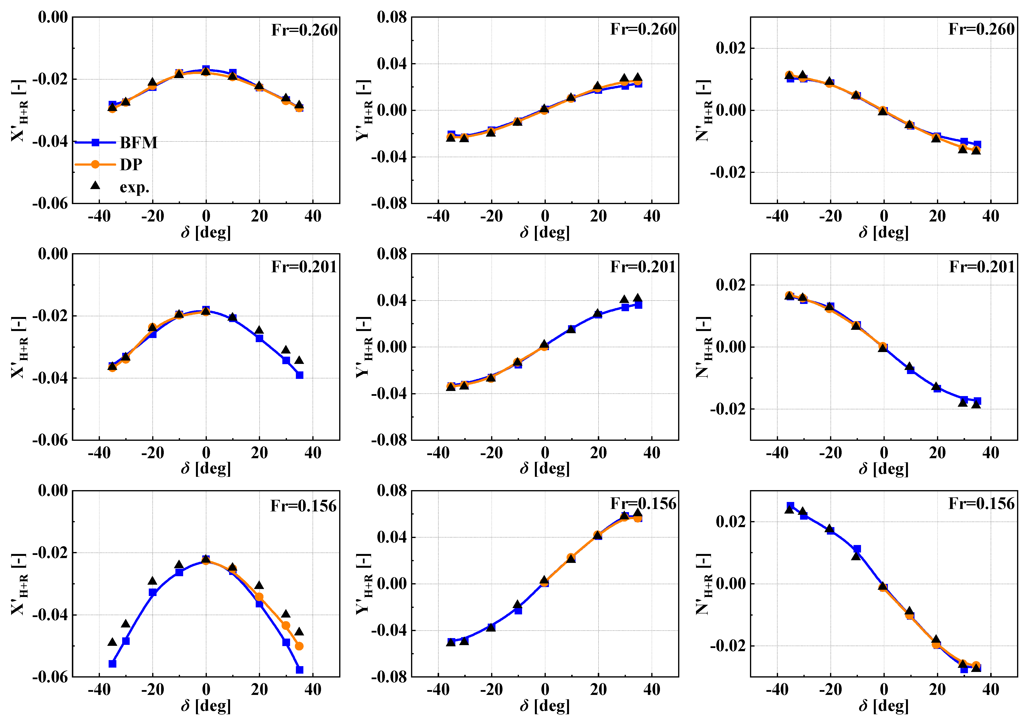
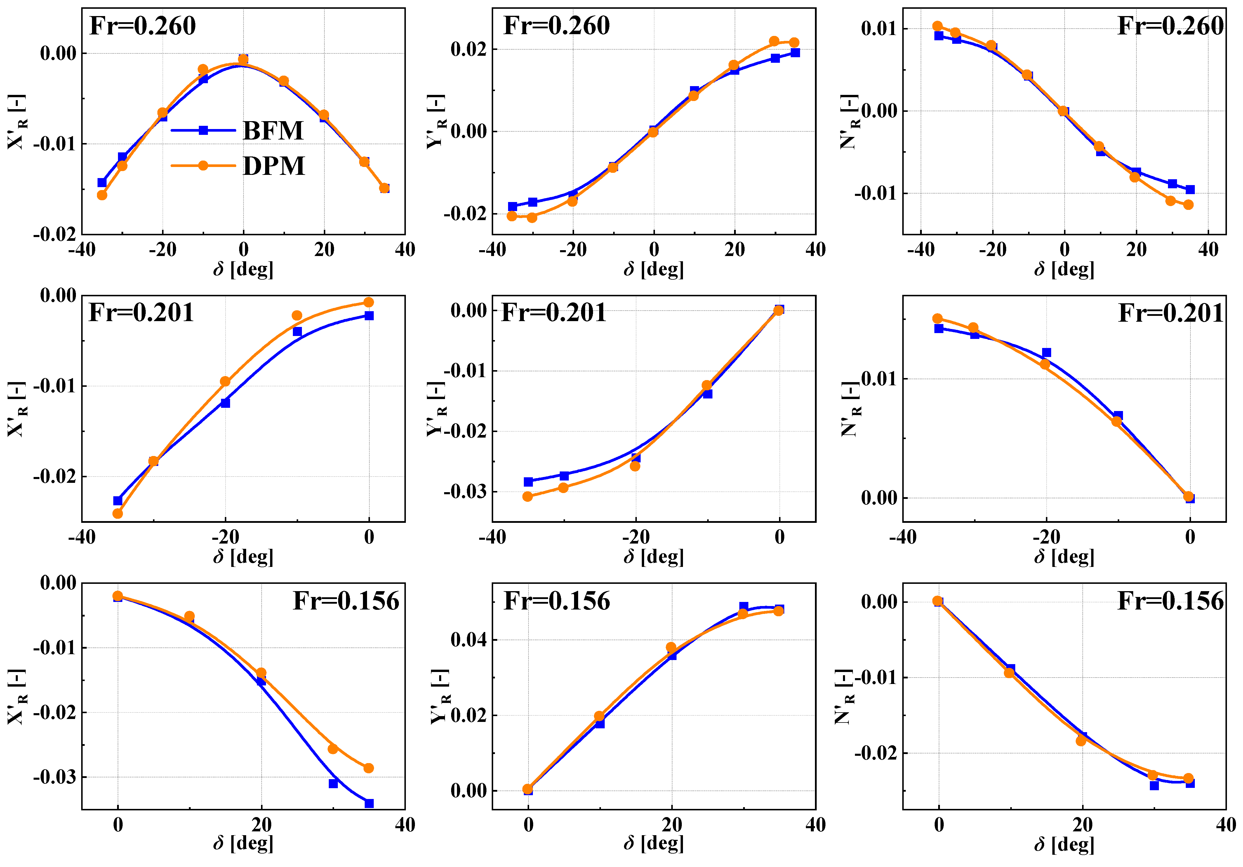
5.1. Static Rudder Force

Figure 7 compares EFD data with the computed hull and rudder hydrodynamic forces/moments at three different Fr numbers for the rudder force case.
Note that for the simulations using DPM at F r = 0.201 and F r = 0.156 , only the partial cases with δ 0 or δ 0 are computed. For the simulations using both propulsion models, the error in the prediction of X H + R at F r = 0.260 is large at small rudder angles, since the value of the total longitudinal force on the hull is inherently small at the self-propelled point of rotation speed. On the whole, the results of the DPM are in good agreement with the experimental data. The results of the BFM for X H + R at a large rudder angle (>20 deg) for the lowest speed ( F r = 0.156 ) are different from the experimental data, and, with the increase in F r , the prediction of the BFM for X H + R is closer to the experimental data. The influence of δ is well captured at the linear region, while at the larger rudder angle for the highest speed ( F r = 0.260 ), the differences between the results of the BFM for Y H + R and N H + R and the experimental data are beyond 10%.
This error may be due to the simple propeller model of the BFM. The propeller’s inflow is strongly affected by the wake of the hull. In the case of a lower speed or a larger rudder angle, the wake of the ship undergoes significant changes due to the more obvious flow separation in these cases. Specifically, variations in fluid velocity influence the stability of the boundary layer. An increase in fluid velocity enhances the fluid momentum within the boundary layer, thereby inhibiting flow separation. In contrast, the rudder angle primarily affects the adverse pressure gradient in the ship’s wake. A larger rudder angle intensifies the adverse pressure gradient, making flow separation more likely to occur. And this simple propeller model cannot truly represent the propeller load under this actual working condition. Therefore, it cannot accurately give the eroding velocity of the propeller wake on the rudder and then affect the hydrodynamic force and moment acting on the rudder.
Figure 8 shows a comparison of the hydrodynamic forces and moments on the rudder computed by the BFM and DPM simulations. Their trends and differences are very similar to those results in Figure 7. And the differences in the hydrodynamic prediction of the hull–propeller–rudder system are mainly caused by differences in the hydrodynamic prediction acting on the rudder.
The pressure-distribution prediction on the hull and rudder using two propulsion models is further explored (see Figure 9). For the BFM and DPM propulsion model simulations F r = 0.260 and δ = 35 deg, the hull pressure-distribution predictions are similar, with differences mainly in the rudder. This aligns with the transverse force and yaw moment predictions in Figure 7 and Figure 8. Differences in the hydrodynamic predictions of the ship–propeller–rudder system from the RANS simulations based on the BFM and the DPM are mainly due to discrepancies in the hydrodynamic predictions on the rudder. As analyzed earlier, this is largely because the adopted body-force model cannot accurately capture the influence of the propeller on the rudder.
Figure 10 shows the local streamlines through the propeller panel and the pressure distributions on the rudder at F r = 0.260 and δ = 35 deg. It can be observed that the BFM is similar to the DPM in predicting the trend of the wake in general. However, the BFM cannot predict the hub vortex (dashed cycle) of the propeller very well due to the absence of a propeller root, which leads to the differences in the prediction of the low-pressure area in the middle of the rudder upstream surface compared to the DPM. Obviously, since the propeller surface does not actually exist in the BFM, it cannot predict the slight vortices emitted by the propeller blade tip (dashed cycle), which leads to the inaccurate prediction of the low-pressure area at the upper and lower ends of the rudder. This makes the BFM underestimate the hydrodynamic forces on the rudder. Since the partially vortex-induced differences with the predicted results using the DPM are negative values, the differences can be recorded as Δ X v o r t e x and Δ Y v o r t e x .
Figure 11 shows propeller vortices represented by a helicity of 40 at different ship speeds and rudder angles. And the swirl of the wake flow for both the DPM- (top) and BFM (bottom)-driven simulations can be observed. The difference between them also increases with an increase in the rudder angle. In simulations driven by the DPM and BFM, there are differences in the rotation of the wake. For instance, DPM can predict the spiral shape of the tip vortices of the propeller, while BFM cannot capture this phenomenon. As the rudder angle increases, the differences between the two models become more significant. This indicates that maneuvering motion has an essential effect on the generation and development of vortices in the propeller wake.
As previously mentioned, the adopted BFM model cannot provide the actual propeller thrust under real operating conditions. Therefore, it is necessary to examine the discrepancy between the thrust and torque predicted by the BFM model and the actual values. The thrust and torque generated by the two models at different speeds and rudder angles are investigated, as shown in Figure 12. The DPM’s prediction of thrust and torque is very close to the test value. While the thrust and torque predicted by this simple BFM model are fixed at a fixed ship speed, leading to the difference in the prediction of flow velocity in the wake field accelerated by the propeller compared to DPM. This is the second reason for its inaccurate prediction of how hydrodynamic forces act on the rudder. This difference caused by inflow velocity can be recorded as Δ X v e l o c i t y and Δ Y v e l o c i t y . They are small values when the difference between T and Q is small (below 10%) and large when the difference between T and Q is large (over 10%).
Figure 13 shows the pressure on the stern region and the velocity magnitude at the central longitudinal section for different ship speeds and rudder angles. Overall, the pressure and axial velocity distributions are similar for both propulsion methods. When the rudder angle is small ( δ = 10 deg), a high-pressure region exists in the upper half of the port-leading edge of the rudder. Further downstream, the pressure gradually decreases as the rudder thickness decreases, and at the trailing edge of the rudder, the pressure rises again. Correspondingly, a low-pressure zone exists in the lower half of the port-leading edge of the rudder, where the pressure gradually increases as the thickness of the rudder decreases. For the starboard portion of the rudder, the pressure distribution is just the opposite. There is a low-pressure zone in the upper half of the starboard-leading edge of the rudder and a high-pressure zone in the lower half of the leading edge. As the rudder angle increases ( δ = 35 deg), the lower half of its port-leading edge changes from a low-pressure zone to a high-pressure zone, while the corresponding lower half of the starboard-leading edge changes from a high-pressure zone to a low-pressure zone. As speed increases, the area of the high-pressure and low-pressure zones increases.
Under different maneuvering conditions, the induced velocity by the BFM is sometimes greater than that predicted by the DPM (Figure 13a), and sometimes less than the induced velocity obtained by the DPM (Figure 13b,c). These observations are congruent with the thrust predictions presented in Figure 12. The former leads to a larger hydrodynamic force on the rudder obtained by the BFM, while the latter leads to a smaller hydrodynamic force on the rudder obtained by the BFM, which can be respectively recorded as Δ X v e l o c i t y and Δ X v e l o c i t y .
To sum up, we can simply analyze the differences in how the predicted forces and moments act on the rudder between the BFM and DPM under different rudder angles and ship speeds. When F r = 0.156 and δ = 10 deg, the prediction value is lower due to the inaccurate prediction of the propeller hub vortex and slight vortex by the BFM. Under this condition, the differences with the DPM are small negative values, which are recorded as Δ X v o r t e x s m a l l and Δ Y v o r t e x s m a l l . And the predictions of T and Q by the BFM are higher than that by DPM, which leads to more severe scouring of the high-pressure area on the upstream surface of the propeller and rudder. This part makes its prediction of longitudinal force and transverse force higher than that of the DPM. Because the differences are small positive values, they can be recorded as Δ X v e l o c i t y s m a l l and Δ Y v e l o c i t y s m a l l . The equation Δ X v o r t e x s m a l l + Δ X v e l o c i t y s m a l l 0 makes the prediction of longitudinal force close to that of the DPM. For the transverse force, there is a similar calculation, Δ Y v o r t e x s m a l l + Δ Y v e l o c i t y s m a l l 0 , making the prediction close. For the yaw moment, the moment of the transverse force on the rudder predicted by the BFM to the center point of the hull is also close to the transverse force on the rudder predicted by the DPM.
Furthermore, when F r = 0.260 and δ = 35 deg, the prediction value is smaller due to the inaccurate prediction of the propeller hub vortex and the slight vortex by the BFM. Under this condition, the differences from the DPM are large negative values, which are recorded as Δ X v o r t e x l arg e and Δ Y v o r t e x l arg e . And the predictions of T and Q by the BFM are smaller than that of the DPM, which leads to less severe scouring of the high-pressure area on the upstream surface of the propeller and rudder. This part makes its prediction of longitudinal force and transverse force smaller than that of the DPM. Because the differences are small negative values, they can be recorded as Δ X v e l o c i t y s m a l l and Δ Y v e l o c i t y s m a l l . There is a Δ X v o r t e x l arg e Δ X v e l o c i t y s m a l l < 0 and Δ Y v o r t e x l arg e Δ Y v e l o c i t y s m a l l < 0 . At this point, the yaw moment predicted by the BFM, namely the moment of the lateral force on the rudder about the ship’s center, is smaller than that predicted by the DPM. The above analysis confirms the differences and accuracy in the predictions shown in Figure 7 and Figure 8, further highlighting the drawbacks of the employed body-force model. These analyses are consistent with the results in Figure 7 and Figure 8, and can also be extended to other rudder angles, which will not be listed here.
Figure 14 shows the longitudinal velocity distribution of the BFM and DPM immediately ahead and behind the rudder in the case of F r = 0.260 and δ = 35 deg. Both of them can capture the vorticity at the right rear of the hull (shown by the dotted line), although there are differences in size. However, the DPM captured the vortex in the upper half of the rudder (as shown in the implementation), which is not observed in the BFM results. Viewed from the ship’s stern towards the bow, at a rudder angle of 35 deg, even with a zero-drift angle, the rudder forms an angle with the flow, generating lateral flow at the stern. The stern’s complex shape causes a stern bilge vortex to form in the lower-left area. High-energy fluid particles in the boundary layer continue to flow past the rudder, creating a large vortex at the stern’s starboard side. Low-energy particles move away from the hull, increasing the wake thickness. Near the rudder’s leading edge, fluid particles experience significant velocity changes and gradients, causing the boundary layer thickness to increase rapidly at the stern and over the rudder, reducing frictional stress at the stern. The large rudder angle increases the adverse pressure gradient, further thickening the boundary layer, reducing frictional stress on the rudder, and causing noticeable flow separation, which changes the frictional stress distribution, reducing it after separation while increasing form drag. At low speeds and large rudder angles, form drag dominates, reducing frictional stress and increasing form drag, which enlarges the BFM’s longitudinal force prediction error. At high speeds, the frictional stress proportion decreases, and form drag increases. Higher speeds suppress flow separation, reduce frictional stress, and increase form drag, yet the BFM’s longitudinal force prediction error diminishes.

5.2. Static Drift Motion with Rudder Deflection

Figure 15 shows the comparison of computed forces and moments on the hull and rudder for CFD and EFD in the static drift motion with rudder deflection.
Note that only the conditions at the lowest speed ( F r = 0.156 ) and the maximum drift angle ( β = 12 deg) are simulated for the DPM. Generally speaking, the DPM’s results are found to be more aligned with the experimental data. In the case of the body simulations using the BFM, the predictions for Y H + R and N H + R are more accurate in comparison to X H + R . Furthermore, these BFM-based predictions show a higher degree of correspondence with experimental data at higher speed ( F r = 0.201 ), with smaller drift angles ( β = ± 4 deg) and smaller rudder angles. In other words, as the drift and rudder angles increase, the discrepancy between the RANS simulation results based on the BFM and the experimental values grows.
The comparisons of the hydrodynamic forces and moments acting on the rudder between the simulations based on the BFM and DPM at F r = 0.156 and β = 12 deg are given in Figure 16. Their trends and differences are very similar to those in Figure 15, indicating that the difference between the two models in predicting the forces and moments of the hull–propeller–rudder system is mainly reflected in the rudder in the drift and rudder motion. This is similar to the situation under the rudder motion.
The thrust and torque of the propellers for CFD and EFD at F r = 0.156 and β = 12 deg are compared in Figure 17. Similar to the rudder deflection, the results of the DPM are very close to the experimental data. The thrust and torque of the BFM are fixed values at a fixed speed and drift angle, which are greater than the results of both the DPM and EFD. And the difference between the results from the BFM and DPM is larger than that of the rudder deflection. In fact, the incident flow ahead of the propeller varies with the drift angle, which affects the load acting on the propeller. This is the reason leading to the differences.
Figure 18 shows the boundary layer at different rudder angles as cross-sections colored with vorticity magnitude. The interaction between the bottom of the hull and the drift velocity produces a strong bilge vortex that interacts with the propeller. The cross-flow vorticity and free-surface pressure distribution at the stern of the ship are obviously different and increase with the increase in the rudder angle. At large rudder angles, enhanced lateral vorticity from flow separation and reattachment at the rudder affects propeller wake characteristics, impacting rudder effectiveness and ship maneuverability. Transverse vorticity development also indicates boundary layer separation. Figure 18 shows that the propeller numerical model mainly influences hull-surface vortices at the rear hull, while the BFM underestimates the interaction between the propeller and hull vortices compared to the DPM. DPM results show that as the rudder angle increases, the interaction between the propeller and hull vortices intensifies, and the stern free surface deforms more, indicating that maneuvering significantly affects the propeller wake field.
Figure 19 shows the longitudinal velocity distribution in front and behind the rudder at F r = 0.156 , β = 12 deg, and δ = 30 deg. There are differences in color depth and area size between the results of the BFM and DPM, although the distributions are similar, and the difference is more obvious at the trailing edge of the rudder. Note that both the DPM and BFM captured the vortex in the upper half of the rudder trailing edge. Figure 19 shows that the propeller numerical model is crucial for the boundary layer on the rudder surface, while the “body-force model” fails to accurately predict the flow field behind the propeller and around the rudder.
Figure 10, Figure 11, Figure 13, Figure 14, Figure 18 and Figure 19 show the complexity of the turbulence in the propeller/rudder region during maneuverings. The flow has generated high-level turbulence on different scales when it reaches the rudder surface, which is initially generated by the interaction between the boundary layer and the bottom of the ship and enhanced by the effect of the propeller. Finally, due to the effect of the rudder, greater differences are formed.

5.3. Static Circular Motion with Rudder Deflection

As shown in Figure 20, the forces and moments on the hull and rudder from the BFM-based simulations (solid lines) and EFD (triangular symbols) across different turning speeds and drift angles are compared. The comparison displays the same trend in terms of numerical accuracy as shown from the comparisons for the static rudder and the static drift and rudder cases. The predicted results are close to the experimental data in general, except for the longitudinal forces at a large rudder angle, where the flow separates strongly on the rudder. The slopes of the five curves of Y H + R are almost the same, the same as those of N H + R . This indicates that the dimensionless lateral force and yaw moment are not sensitive to the return angle speed in the static circular and rudder angle tests. The BFM demonstrates acceptable accuracy within a certain range of maneuvering motions, and its forecast results can be used to determine the hydrodynamic derivatives related to turning rate and the rudder angle.

6. Conclusions

This article presents forced motion (static rudder, static drift, and static circle) simulations based on the BFM and DPM for RANS computations of the KCS model. Verification and validation research for the RANS methods based on both the BFM and DPM in the article has been performed. The computed results are compared with each other and the benchmark experimental data from SIMMAN 2014. The hydrodynamic forces and moments acting on the rudder are compared, and the wake field of the propeller and rudder is analyzed too. The following conclusions can be drawn:
(a)
It is feasible to conduct RANS simulations based on the BFM and DPM to predict the hydrodynamic forces and moments of ship hulls. The results of the DPM are more accurate but more time-consuming, with an average computed time for one case close to 35 times that of BFM. However, the BFM exhibits certain inaccuracies in predicting hydrodynamic forces and moments at large rudder angles and/or drift angles. Its longitudinal force values are more sensitive to the drift angle, turning rate, and ship speed, while transverse forces and yaw moments are more sensitive to the rudder angle.
(b)
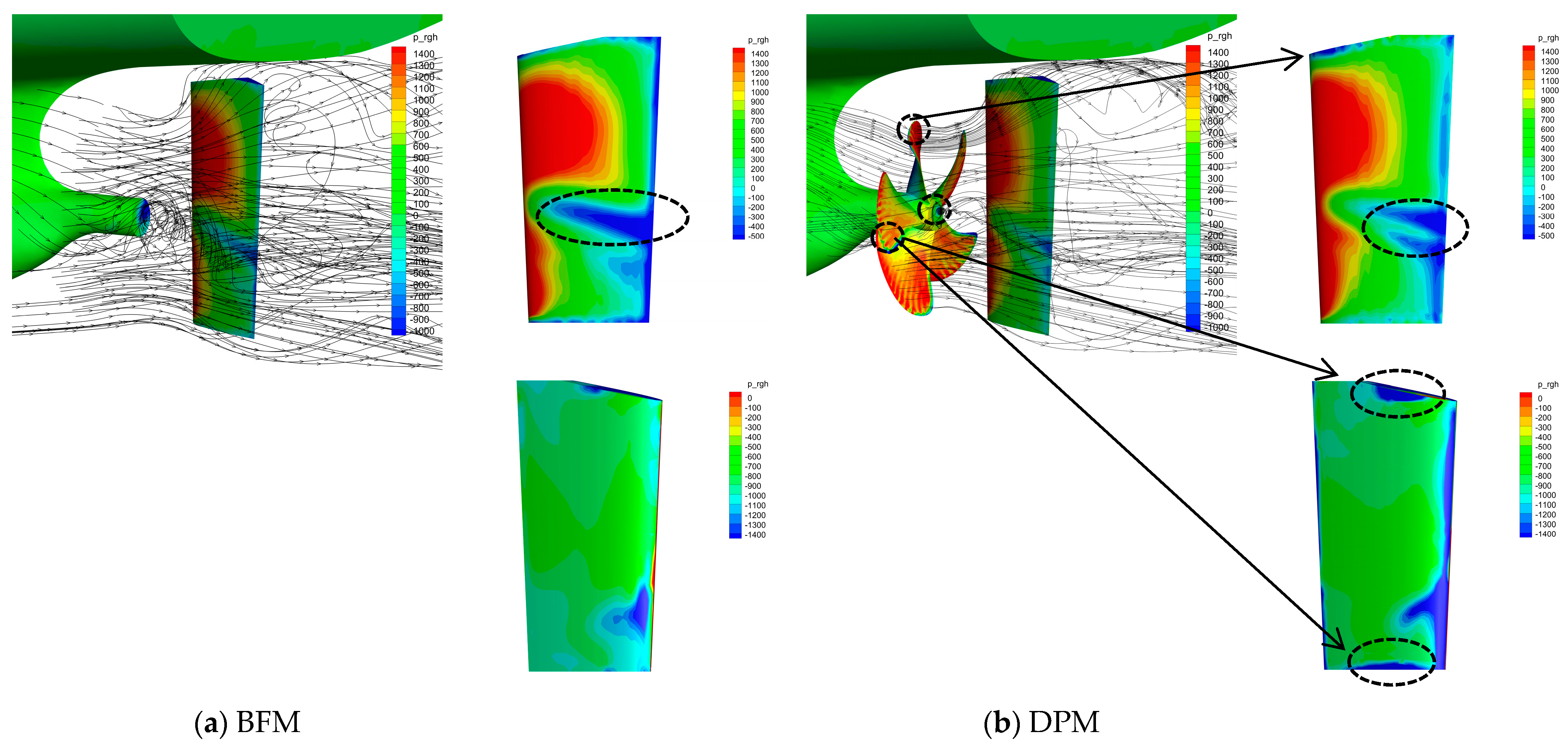
The main reason for the computed difference between the BFM and DPM methods is the difference in wake field, reflected in the difference in the hydrodynamic force and moment acting on the rudder. Furthermore, there are two sources of error for the results of the BFM method: One is the lack of a physical shape in propeller blades, which means that there is a lack of lather force on the propeller during rotation, leading to the inability to accurately predict the interaction between the propeller-blade root or blade-tip leakage vortices and the rudder. Another issue is the limitation of the adopted model, which makes it impossible to accurately provide the thrust and torque generated by the propeller under actual cases.
(c)
The BFM would still be sufficient for calculating linear hydrodynamic derivatives related to rudder angle. The DPM method is more advantageous for complex wake-field simulations, even if the BFM method saves a lot of computation time.
Future work includes two aspects. One is to improve this simple BFM method so that it can accurately predict the thrust and torque generated by the propeller under actual working conditions. Another is to obtain hydrodynamic derivatives based on the computed results, compare the differences in hydrodynamic derivatives obtained by these two propulsion methods, and then compare the results of the maneuverability predictions.

Author Contributions

L.J.: methodology, conceptualization, software, formal analysis, visualization, writing—original draft, investigation, validation, and writing—review and editing. J.Y.: writing—review and editing, supervision, conceptualization, and methodology. Z.L.: methodology, funding acquisition, formal analysis, investigation, and software. All authors have read and agreed to the published version of the manuscript.

Funding

This research is supported by the National Natural Science Foundation of China [grant number 551720105011].

Data Availability Statement

The original contributions presented in this study are included in the article. Further inquiries can be directed at the corresponding author.

Conflicts of Interest

The authors declare no conflict of interest.

References

  1. IMO. Standards for Ship Maneuverability. Resolution MSC.137(76). 2002. Available online: https://wwwcdn.imo.org/localresources/en/KnowledgeCentre/IndexofIMOResolutions/MSCResolutions/MSC.137(76).pdf (accessed on 7 April 2025).
  2. Yu, J.; Feng, D.; Liu, L.; Yao, C.; Wang, X. Assessments of propulsion models for free running surface ship turning circle simulations. Ocean Eng. 2022, 250, 110967. [Google Scholar] [CrossRef]
  3. Simonsen, C.D.; Otzen, J.F.; Klimt, C.; Larsen, N.L.; Stern, F. Maneuvering predictions in the early design phase using CFD generated PMM data. In Proceedings of the 29th Symp Naval Hydrodynamics, Gothenburg, Sweden, 26–31 August 2012. [Google Scholar]
  4. Yoon, H.; Simonsen, C.D.; Benedetti, L.; Longo, J.; Toda, Y.; Stern, F. Benchmark CFD validation data for surface combatant 5415 in PMM maneuvers—Part I: Force/moment/motion measurements. Ocean Eng. 2015, 109, 705–734. [Google Scholar] [CrossRef]
  5. Zhang, C.; Liu, X.; Wan, D.; Wang, J. Experimental and numerical investigations of advancing speed effects on hydrodynamic derivatives in MMG model, part I: Xvv, Yv, Nv. Ocean Eng. 2019, 179, 67–75. [Google Scholar] [CrossRef]
  6. Yun, K.; Yeo, D.J.; Kim, D.J. An experimental study on the turning characteristics of KCS with CG variations. In Proceedings of the International Conference on Ship Manoeuvrability and Maritime Simulation (MARSIM 2018), Halifax, NS, Canada, 12–16 August 2018; pp. 12–16. [Google Scholar]
  7. Yeo, D.J.; Yun, K.; Kim, Y.G. A study on the effect of heel angle on maneuvering characteristics of KCS. In Proceedings of the International Conference on Ship Manoeuvrability and Maritime Simulation (MARSIM 2018), Halifax, NS, Canada, 12–16 August 2018; pp. 1–10. [Google Scholar]
  8. Jiang, L.; Yao, J.; Liu, Z. Comparison between the RANS simulations of double-body flow and water–air flow around a ship in static drift and circle motions. J. Marine Sci. Eng. 2022, 10, 970. [Google Scholar] [CrossRef]
  9. Carrica, P.M.; Ismail, F.; Hyman, M.; Bhushan, S.; Stern, F. Turn and zigzag maneuvers of a surface combatant using a URANS approach with dynamic overset grids. J. Mar. Sci. Technol. 2013, 18, 166–181. [Google Scholar] [CrossRef]
  10. Mofidi, A.; Carrica, P.M. Simulations of zigzag maneuvers for a container ship with direct moving rudder and propeller. Comput. Fluids 2014, 96, 191–203. [Google Scholar] [CrossRef]
  11. Carrica, P.M.; Mofidi, A.; Eloot, K.; Delefortrie, G. Direct simulation and experimental study of zigzag maneuver of KCS in shallow water. Ocean Eng. 2016, 112, 117–133. [Google Scholar] [CrossRef]
  12. Prandtl, L. Über die ausgebildete Turbulenz. ZAMM 1925, 5, 136–139. [Google Scholar] [CrossRef]
  13. Jin, Y.; Duffy, J.; Chai, S.; Magee, A.R. DTMB 5415M dynamic manoeuvres with URANS computation using body-force and discretised propeller models. Ocean Eng. 2019, 182, 305–317. [Google Scholar] [CrossRef]
  14. Wang, J.; Wan, D.; Yu, X. Standard zigzag maneuver simulations in calm water and waves with direct propeller and rudder. In Proceedings of the ISOPE International Ocean and Polar Engineering Conference (ISOPE 2017), San Francisco, CA, USA, 25 June–1 July 2017; pp. 1042–1048. [Google Scholar]
  15. Cura-Hochbaum, A. Virtual PMM tests for maneuvering prediction. In Proceedings of the 26th Symposium on Naval Hydrodynamics, Rome, Italy, 17–22 September 2006. [Google Scholar]
  16. Duman, S.; Bal, S. Prediction of maneuvering coefficients of Delft Catamaran 372 hull form. In Proceedings of the 18th International Congress of the International Maritime Association of the Mediterranean (IMAM 2019), Varna, Bulgaria, 9 September 2019; pp. 167–174. [Google Scholar]
  17. Visonneau, M.; Guilmineau, E.; Rubino, G. Computational analysis of the flow around a surface combatant at 10° static drift and dynamic sway conditions. In Proceedings of the 32nd ONR Symposium, Hamburg, Germany, 5–10 August 2018; pp. 5–10. [Google Scholar]
  18. Islam, H.; Guedes Soares, C. Estimation of hydrodynamic derivatives of a container ship using PMM simulation in OpenFOAM. Ocean Eng. 2018, 164, 414–425. [Google Scholar] [CrossRef]
  19. Silva, K.M.; Aram, S. Generation of hydrodynamic derivatives for ONR Topside Series using computational fluid dynamics. In Proceedings of the STAB 2018, Kobe, Japan, 16–21 September 2018; pp. 16–21. [Google Scholar]
  20. Sukas, O.F.; Kinaci, O.K.; Bal, S. System-based prediction of maneuvering performance of twin-propeller and twin-rudder ship using a modular mathematical model. Appl. Ocean Res. 2019, 84, 145–162. [Google Scholar] [CrossRef]
  21. Sakamoto, N.; Ohashi, K.; Araki, M.; Kume, K.; Kobayashi, H. Identification of KVLCC2 manoeuvring parameters for a modular-type mathematical model by RaNS method with an overset approach. Ocean Eng. 2019, 188, 106257. [Google Scholar] [CrossRef]
  22. Castro, A.M.; Carrica, P.M.; Stern, F. Full scale self-propulsion computations using discretized propeller for the KRISO container ship KCS. Comput. Fluids 2011, 51, 35–47. [Google Scholar] [CrossRef]
  23. Stern, F.; Yang, J.M. Computational ship hydrodynamics: Nowadays and way forward. Int. Shipbuild. Prog. 2013, 60, 3–105. [Google Scholar] [CrossRef]
  24. Pankajakshan, R.; Remotigue, S.; Taylor, L.; Jiang, M.; Briley, W.; Whitfield, D. Validation of control-surface induced submarine maneuvering simulations using UNCLE. In Proceedings of the 24th Symp Naval Hydrodynamics, Fukuoka, Japan, 8–13 July 2002. [Google Scholar]
  25. Cura-Hochbaum, A.; Uharek, S. Prediction of the Maneuvering Behavior of the KCS Based on Virtual Captive Tests; TU: Berlin, Germany, 2014. [Google Scholar]
  26. Carrica, P.M.; Sadat-Hosseini, H.; Stern, F. CFD analysis of broaching for a model surface combatant with explicit simulation of moving rudders and rotating propellers. Comput. Fluids 2012, 53, 117–132. [Google Scholar] [CrossRef]
  27. Hough, G.R.; Ordway, D.E. The generalized actuator disk. Dev. Theor. Appl. Mech. 1965, 2, 317–336. [Google Scholar]
  28. Ohashi, K.; Kobayashi, H.; Hino, T. Numerical simulation of the free-running of a ship using the propeller model and dynamic overset grid method. Ship Technol. Res. 2018, 65, 153–162. [Google Scholar] [CrossRef]
  29. Bekhit, A.S. Numerical simulation of the ship self-propulsion prediction using body force method and fully discretized propeller model. IOP Conf. Ser. Mater. Sci. Eng. 2018, 400, 042004. [Google Scholar] [CrossRef]
  30. Win, Y.N.; Wu, P.C.; Akamatsu, K.; Okawa, H.; Stern, F.; Toda, Y. RANS Simulation of KVLCC2 using Simple Body-Force Propeller Model With Rudder and Without Rudder. J. Jpn. Soc. Nav. Archit. Ocean Eng. 2016, 23, 1–11. [Google Scholar]
  31. Aram, S.; Mucha, P. Computational fluid dynamics analysis of different propeller models for a ship maneuvering in calm water. Ocean Eng. 2023, 276, 114226. [Google Scholar] [CrossRef]
  32. Feng, D.; Yu, J.; He, R.; Zhang, Z.; Wang, X. Improved body force propulsion model for ship propeller simulation. Appl. Ocean Res. 2020, 104, 102328. [Google Scholar] [CrossRef]
  33. Yao, J.; Liu, Z.; Song, X.; Su, Y. Ship manoeuvring prediction with hydrodynamic derivatives from RANS: Development and application. Ocean Eng. 2021, 231, 109036. [Google Scholar] [CrossRef]
  34. Menter, F.R.; Kuntz, M.; Langtry, R. Ten years of industrial experience with the SST turbulence model. In Proceedings of the Turbulence, Heat and Mass Transfer 4, Antalya, Turkey, 12–17 October 2003. [Google Scholar]
  35. Hirt, C.W.; Nichols, B.D. Volume of fluid (VOF) method for the dynamics of free boundaries. J. Comput. Phys. 1981, 39, 201–225. [Google Scholar] [CrossRef]
  36. Stern, F.; Kim, H.T.; Patel, V.C.; Chen, H.C. Computation of viscous flow around propeller-shaft configurations. J. Ship Res. 1988, 32, 263–284. [Google Scholar] [CrossRef]
  37. Simonsen, C.D. KCS PMM test with appended hull, FORCE 2009-SIMMAN 2014. In Proceedings of the Workshop on Verification and Validation of Ship Manoeuvring Simulation Methods, Copenhagen, Demark, 8–10 December 2014. [Google Scholar]
  38. Stern, F.; Wilson, R.V.; Coleman, H.V.; Paterson, E.G. Comprehensive approach to verification and validation of CFD simulations—Part 1 and 2: Methodology and procedures. ASME J. Fluids Eng. 2001, 124, 793–802. [Google Scholar] [CrossRef]
  39. ITTC. Practical Guidelines for Ship CFD Applications. ITTC Recommended Procedures and Guidelines. 7.5-03-02-03. 2014. Available online: https://www.ittc.info/media/8165/75-03-02-03.pdf (accessed on 7 April 2025).
  40. Yao, J.; Jin, W.; Song, Y. RANS simulation of the flow around a tanker in force motion. Ocean Eng. 2016, 127, 236–245. [Google Scholar] [CrossRef]
Figure 1. Computational domain and boundaries.
Jmse 13 00788 g001
Figure 2. The geometry of a KCS with a rudder and propeller.
Jmse 13 00788 g002
Figure 3. Computational domain and the refinement grid on the free surface.
Jmse 13 00788 g003
Figure 4. Grids in the computational region: (a) hull; (b) bow; and (c) stern and rudder.
Jmse 13 00788 g004
Figure 5. Two propulsion strategies at the stern of the KCS.
Jmse 13 00788 g005
Figure 6. Grid space. (Left): external static part (stern); (middle): internal dynamic part (BFM); (right): internal dynamic part (DPM).
Jmse 13 00788 g006
Figure 7. Comparisons of hydrodynamic forces and moments on the hull and rudder from CFD and EFD for the static rudder case.
Jmse 13 00788 g007
Figure 8. Comparisons of hydrodynamic forces and moments on the rudder from the CFD for the static rudder case.
Jmse 13 00788 g008
Figure 9. Comparisons of pressure distributions on the hull and rudder from CFD for the static rudder case. (Top: BFM; bottom: DPM; left: starboard; and right: port).
Jmse 13 00788 g009
Figure 10. Local streamlines through the propeller panel and the pressure distributions on the rudder. ((a): BFM; (b): DPM).
Jmse 13 00788 g010
Figure 11. Comparison of propeller vortices represented by a helicity of 40 at different F r and rudder angles for the DPM- (top) and BFM (bottom)-driven simulations. ((a) F r = 0.156 , δ = 10 deg; (b) F r = 0.260 , δ = 35 deg; and (c) F r = 0.156 , δ = 35 deg).
Jmse 13 00788 g011
Figure 12. Propeller thrust and torque from CFD and EFD at different speeds and rudder angles. (Top: thrust; bottom: torque).
Jmse 13 00788 g012
Figure 13. Comparison of the pressure on the stern region and the velocity magnitude on the central longitudinal section at different ship speeds and rudder angles ((a) F r = 0.156 , δ = 10 deg; (b) F r = 0.260 , δ = 35 deg; and (c) F r = 0.156 , δ = 35 deg) for the DPM- (top) and BFM (bottom)-driven simulations.
Jmse 13 00788 g013aJmse 13 00788 g013b
Figure 14. Longitudinal velocity distributions of the BFM (left) and DPM (right) immediately ahead (top) and behind (bottom) the rudder. ( F r = 0.260 and δ = 35 deg).
Jmse 13 00788 g014
Figure 15. Comparison of computed forces and moments on the hull and rudder for CFD and EFD in the static drift motion with rudder deflection.
Jmse 13 00788 g015
Figure 16. Comparison of the computed forces and moments on the rudder at F r = 0.156 and β = 12 deg.
Jmse 13 00788 g016
Figure 17. Propeller thrust and torque from CFD and EFD at F r = 0.156 and β = 12 deg.
Jmse 13 00788 g017
Figure 18. Cross-flow colored with the vorticity magnitude.
Jmse 13 00788 g018aJmse 13 00788 g018b
Figure 19. Longitudinal velocity distributions of the BFM (left) and DPM (right) immediately ahead (top) and behind (bottom) the rudder. ( F r = 0.156 , β = 12 deg, and δ = 30 deg).
Jmse 13 00788 g019aJmse 13 00788 g019b
Figure 20. Comparisons of hydrodynamic forces and moments on the hull and rudder between CFD based on the BFM and EFD for the static circular and rudder deflections.
Jmse 13 00788 g020
Table 1. Constants for the k-ω SST model.
Symbol a 1 β * γ 1 β 1 γ 2 β 2 σ k 1 σ ω 1 σ k 2 σ ω 2
Value0.310.090.5550.0750.440.08280.850.51.00.856
Table 2. Principal particulars of a KCS.
ItemsFull ScaleModel for CFD
Hull
Lpp (m)2304.3671
Lwl (m)232.54.4141
Bwl (m)32.20.6114
D (m)190.4500
T (m)10.80.2051
Displacement (m3)52,0300.3562
CB0.6510.651
CM0.9850.984
LCB (%), fwd+−1.48−1.48
Rudder
S (m2)1150.0415
Lather area (m2)54.450.0196
Propeller
TypeFPFP
No. of blades55
D (m)7.90.150
P/D (0.7R)0.9971.000
Ae/A00.80.700
RotationRight handRight hand
Hub ratio0.180.227
n (rps)-14
Table 3. Computational cases for simulation using the BFM.
Motions F r
[-]
β
[deg]
r
[-]
δ
[deg]
Cases Number
Static rudder0.156000, ±10, ±20,
±30, ±35
27
0.201
0.260
Static drift and rudder0.156−1200, ±10, ±20,
30, 35
14
1200, ±10, ±20,
−30, −35
0.201−400, ±10, ±20,
30, 35
14
4 0, ±10, ±20,
−30, −35
Static circular and rudder0.2010±0.4, ±0.60, ±10, ±20,
±30, ±35
36
Total----91
Table 4. Computational cases for simulation using the DPM.
Motions F r
[-]
β
[deg]
r
[-]
δ
[deg]
Cases Number
Static rudder0.156000, 10, 20,
30, 35
5
0.2010, −10, −20,
−30, −35
5
0.2600, ±10, ±20,
±30, ±35
9
Static drift and rudder0.156−1200, ±20, 30, 355
Total----24
Table 5. Cell numbers (million) and mean y + .
GridExternal Static PartMean
y +
Internal Dynamic Part (BFM)Mean
y +
Internal Dynamic Part (DPM)Mean
y +
Coarse0.5666.510.031.220.211.15
Medium0.9654.730.091.200.381.13
Fine1.8843.330.261.160.761.10
Table 6. Computational grids and time steps employed in the verification study (BFM).
GridNumber of
Elements   ( × 1 0 6 )
Δ t 0.01 L U CFL
(1)0.590.020.0260.025
(2)1.050.010.0260.033
(3)2.140.0050.0260.026
Table 7. Computational grids and time steps employed in the verification study (DPM).
GridNumber of
Elements   ( × 1 0 6 )
Δ t 0.01 L U CFL 1 180 n
(1)0.770.000350.0260.0008830.000397
(2)1.340.000350.0260.0013570.000397
(3)2.640.000350.0260.0018640.000397
Table 8. Results for straight-ahead motion in the systematic grids (BFM).
Grid X H + R Diff. (%) n (rps)
(1)−0.016768-14.0607
(2)−0.0171762.4314.4172
(3)−0.0173360.0914.5658
Table 9. Results for straight-ahead motion in the systematic grids (DPM).
Grid X H + R Diff. (%) n (rps)
(1)−0.016948-14
(2)−0.0174272.8314
(3)−0.0175590.0814
Table 10. Grid uncertainty study for straight-ahead motion (BFM).
Quantity r G R G P G C G δ R E G * ( 1 ) U G C S C U G Convergence
Type
X H + R 2 0.392.711.56−0.59−0.33−0.0174591.25Monotonic
Table 11. Grid uncertainty study for straight-ahead motion (DPM).
Quantity r G R G P G C G δ R E G * ( 1 ) U G C S C U G Convergence
Type
X H + R 2 0.283.722.63−0.29−0.47−0.0176911.22Monotonic
Table 12. Results for straight-ahead motion in the systematic time steps (BFM).
Grid Δ t X H + R Diff. (%)
(3)0.02−0.0180
0.01−0.01753.02
0.005−0.01731.16
Table 13. Time step uncertainty study for straight-ahead motion (BFM).
Quantity r T R T P T C T δ R E T * ( 1 ) U T C S C U T Convergence
Type
X H + R 20.41.321.51.990.99−0.01683.98Monotonic
Table 14. Results for the static drift motion in the systematic grids (BFM).
Grid X H + R Diff. (%) Y H + R Diff. (%) N H + R Diff. (%)
(1)−0.019458-−0.070236-−0.021487
(2)−0.0208447.12−0.0721190.27−0.0222210.34
(3)−0.0210531.00−0.0724830.05−0.0225480.15
Table 15. Results for the static drift motion in the systematic grids (DPM).
Grid X H + R Diff. (%) Y H + R Diff. (%) N H + R Diff. (%)
(1)−0.019777-−0.070592-−0.021126
(2)−0.0204143.22−0.0729113.28−0.02442015.59
(3)−0.0206651.23−0.072115−1.09−0.024000−1.72
Table 16. Grid uncertainty study for the static drift motion (BFM).
Quantity r G R G P G C G δ R E G * ( 1 ) U G C S C U G Convergence
Type
X H + R 2 0.511.930.96−3.44−0.15−0.0217943.75Monotonic
Y H + R 2 0.194.744.17−0.12−0.38−0.0728640.88Monotonic
N H + R 2 0.492.331.24−1.17−0.28−0.0228261.74Monotonic
Table 17. Grid uncertainty study for the static drift motion (DPM).
Quantity r G R G P G C G δ R E G * ( 1 ) U G C S C U G Convergence
Type
X H + R 2 0.392.691.54−0.79−0.42−0.0209161.64Monotonic
Y H + R 2 −0.34-----−1.61Oscillatory
N H + R 2 −0.13-----−6.86Oscillatory
Table 18. Validation of the RANS simulation. ( E , U G , U T , U S N , U D , and U V are %EFD).
MotionQuantity S 3 E F D E U G U T U S N U D U V
Straight-
ahead
X H + R (BFM)−0.0173−0.0179−3.351.213.854.0356.42
X H + R (DPM)−0.0176−0.0179−1.681.20-1.2055.14
Drift X H + R (BFM)−0.0211−0.02052.933.864.105.6257.53
Y H + R (BFM)−0.0725−0.0726−0.140.883.974.0756.45
N H + R (BFM)−0.0226−0.0241−6.221.633.734.0756.45
X H + R (DPM)−0.0207−0.02050.981.66-1.6655.27
Y H + R (DPM)−0.0721−0.0726−0.69−1.60-−1.6055.25
N H + R (DPM)−0.0240−0.0241−0.41−6.83-−6.8358.47
Disclaimer/Publisher’s Note: The statements, opinions and data contained in all publications are solely those of the individual author(s) and contributor(s) and not of MDPI and/or the editor(s). MDPI and/or the editor(s) disclaim responsibility for any injury to people or property resulting from any ideas, methods, instructions or products referred to in the content.

