Comparison of Surface Current Measurement Between Compact and Square-Array Ocean Radar

Abstract

High-frequency (HF) ocean radars have become essential tools for monitoring surface currents, offering real-time, wide-area coverage with cost-effectiveness. This study compares the compact CODAR system (MABT, 13 MHz) and the square-array phased-array radar (KNTN, 8 MHz) deployed at Cape Maobitou, Taiwan. Radial velocity measurements were evaluated against data from the Global Drifter Program (GDP), and a quality control (QC) mechanism was applied to improve the data’s reliability. The results indicated that KNTN provides broader spatial coverage, whereas MABT demonstrates higher precision in radial velocity measurements. Baseline velocity comparisons between MABT and KNTN revealed a correlation coefficient of 0.77 and a root-mean-square deviation (RMSD) of 0.23 m/s, which are consistent with typical values reported in previous radar performance evaluations. Drifter-based velocity comparisons showed an initial correlation of 0.49, with an RMSD of 0.43 m/s. In more stable oceanic regions, the correlation improved to 0.81, with the RMSD decreasing to 0.24 m/s. To clarify, this study does not include multiple environmental scenarios but focuses on cases where both radar systems operated simultaneously and where surface drifter data were available within the overlapping area. Comparisons are thus limited by these spatiotemporal conditions. Radar data may still be affected by environmental or human factors, such as ionospheric variations, interference from radio frequency management issues, or inappropriate parameter settings, which could reduce the accuracy and consistency of the observations. International ocean observing programs have developed quality management procedures to enhance data reliability. In Taiwan, the Taiwan Ocean Research Institute (TORI) has established a data quality management mechanism based on international standards for data filtering, noise reduction, and outlier detection, improving the accuracy and stability of radar-derived velocity measurements.To eliminate the effects caused by different center frequencies between MABT and KNTN, this study used the same algorithms and parameter settings as much as possible in all steps, from Doppler spectra processing to radial velocity calculation, ensuring the comparability of the data. This study highlights the strengths and limitations of compact and phased-array HF radar systems based on co-observed cases under consistent operational conditions. Future research should explore multi-frequency radar integration to enhance spatial coverage and measurement precision, improving real-time coastal current monitoring and operational forecasting.

1. Introduction

1.1. Background

Global warming has significantly impacted oceanic systems, which play a crucial role in regulating long-term atmospheric variability. Oceans contribute water vapor and heat to the atmosphere, while atmospheric circulation generates wind stress that drives ocean surface currents, acting as a primary external force in ocean dynamics. Over the past few decades, extensive ocean monitoring efforts have been undertaken by global scientific institutions through programs such as RAPID-AMOC, TOPS, CLIVAR, GO-SHIP, and Argo. These studies have consistently indicated anomalies in global circulation systems due to climate change.

Long-term oceanic observational data are essential for statistical analysis and real-time modeling, improving our ability to predict climate variability. Traditional ocean monitoring techniques such as in situ ship-based observations, drifting and moored buoys, and remote sensing via satellites have inherent limitations. Lagrangian methods are challenged by time-dependent changes in observation points, while Eulerian methods, although capable of fixed-point long-term monitoring, are limited in spatial coverage.

To address the need for wide-area and high-frequency ocean current observations, high-frequency (HF) radar technology has emerged as a cost-effective and efficient solution. It provides near-real-time, large-scale spatial coverage and is relatively inexpensive for long-term monitoring.

Since its theoretical foundation was laid by Crombie (1955) [1], HF radar technology has evolved into a robust tool for oceanographic research (Figure 1). His work on Doppler shifts in first-order Bragg scattering peaks established the basis for surface current measurements, which was later refined by researchers such as Barrick (1972) [2,3], leading to the advancement of over-the-horizon radar technology (Figure 2). Today, HF radars operating within the 3–30 MHz range are widely used for long-term ocean current observations.

Understanding the accuracy and coverage of high-frequency (HF) ocean radar systems is crucial for effective coastal current monitoring and operational forecasting. High-frequency ground-wave radars are mainly classified into narrow-beam and wide-beam systems. Narrow-beam radars, such as Germany’s WERA, the UK’s OSCR, and Canada’s HF-GWR, employ phased-array designs, offering high spatial resolution and accuracy. However, their large antenna arrays and high transmission power requirements pose significant installation challenges. On the other hand, wide-beam radars, represented by the SeaSonde system developed by CODAR in the United States, use whip antennas that are compact, require less installation space, and are highly mobile. Although they have lower azimuthal resolution compared to phased-array systems, their advantages in cost-effectiveness and ease of deployment have driven the rapid development of ocean radar technology worldwide (Figure 3).

Furthermore, many countries’ research institutions and observation networks have deployed non-commercial high-frequency radar systems for studying tides, waves, and ocean dynamics. According to Roarty et al. (2019) [4], global academic, governmental, and private organizations have established regional or national high-frequency radar networks to support coastal scientific and operational activities. As of 2019, approximately 400 radar stations worldwide are operational, providing real-time surface current data. In the Asia–Pacific region alone, there are about 140 active systems, with further growth anticipated due to new installations in countries like the Philippines and Vietnam.

Figure 1. Schematic representation of HF-band radio wave transmission and Bragg resonance effect (adapted from Barrick et al., 1977 [5]).

Figure 1. Schematic representation of HF-band radio wave transmission and Bragg resonance effect (adapted from Barrick et al., 1977 [5]).

Figure 2. The horizontal axis represents the relative frequency (i.e., the transmitted radar frequency is subtracted, so the central frequency is zero). (Top) In the absence of ocean currents, energy peaks in the radar echo frequency spectrum appear symmetrically on both sides of zero frequency, corresponding to ocean waves with a wavelength of λ/2. (Bottom) When ocean currents are present, the Doppler effect induces a frequency shift in the wave spectrum. As a result, the energy peak positions are displaced. If the current flows toward the radar antenna with a velocity Vcr, the frequency shift is given by Δf = (2V_cr)/λ (adapted from Barrick et al., 1977 [5]).

Figure 2. The horizontal axis represents the relative frequency (i.e., the transmitted radar frequency is subtracted, so the central frequency is zero). (Top) In the absence of ocean currents, energy peaks in the radar echo frequency spectrum appear symmetrically on both sides of zero frequency, corresponding to ocean waves with a wavelength of λ/2. (Bottom) When ocean currents are present, the Doppler effect induces a frequency shift in the wave spectrum. As a result, the energy peak positions are displaced. If the current flows toward the radar antenna with a velocity Vcr, the frequency shift is given by Δf = (2V_cr)/λ (adapted from Barrick et al., 1977 [5]).

Figure 3. Development of high-frequency radar (HFR) networks from 2004 to 2022, based on Roarty et al. (2019) [4]: (A) Number of radar stations reported to the U.S. national network (2004–2018). (B) Evolution of HFR systems in Europe (2004–2022). Red indicates systems that are no longer operational, yellow represents future deployments, and green denotes systems currently in operation.

Figure 3. Development of high-frequency radar (HFR) networks from 2004 to 2022, based on Roarty et al. (2019) [4]: (A) Number of radar stations reported to the U.S. national network (2004–2018). (B) Evolution of HFR systems in Europe (2004–2022). Red indicates systems that are no longer operational, yellow represents future deployments, and green denotes systems currently in operation.

In addition, the accuracy and stability of HF radar surface current observations can be affected by environmental and technical factors, such as ionospheric disturbances, radio frequency interference, and inappropriate parameter settings, which may lead to uncertainties in velocity retrieval (Wang et al., 2017) [6]. To ensure data quality, many international observation programs have developed real-time quality control (QC) frameworks for HF radar networks (Roarty et al., 2014; Haines et al., 2017) [7,8]. In Taiwan, the Taiwan Ocean Research Institute (TORI) has established a QC mechanism based on the U.S. IOOS-QARTOD guidelines (U.S. IOOS, 2016) [9], incorporating domestic operational experience (Lai et al., 2015) [10] and international research insights (Kirincich et al., 2012) [11]. This QC framework involves standardized procedures for data filtering, noise reduction, and outlier detection, effectively improving the reliability and consistency of HF radar-derived velocity measurements.

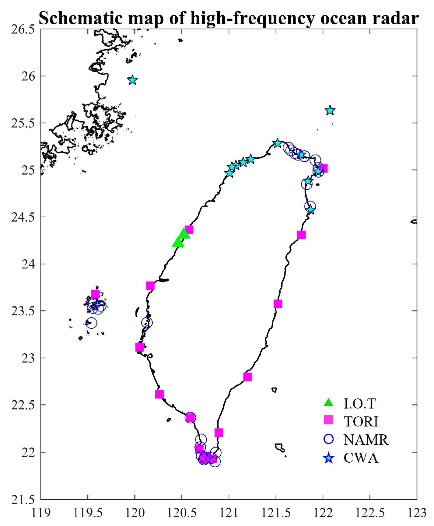
1.2. Introduction of High-Frequency Ocean Radars in Taiwan

While HF radar networks have been extensively developed worldwide, Taiwan’s unique geographic and oceanographic conditions necessitate localized performance assessments of different radar configurations.

Although HF radar technology has been extensively developed worldwide, regional variations in environmental conditions and radar configurations require localized performance evaluations.

Taiwan’s deployment of HF ocean radars began in 2008 through collaboration between Chinese-American scientists at the U.S. Office of Naval Research (ONR) and domestic academic experts. The Ministry of Science and Technology launched the “Coastal Radar Current Observation around Taiwan” project, which was assigned to the TORI. After evaluation, the project adopted the SeaSonde system developed by CODAR, which features an integrated antenna design and direction-finding (DF) technology.

By 2015, Taiwan had completed its nationwide coastal radar observation network, consisting of 12 stations operating at 5 MHz and 5 stations at 13/24 MHz. To address nearshore blind spots, an additional radar station was deployed in Fangliao in 2017, enhancing current data coverage in the coastal waters near Xiaoliuqiu and Pingtung (Figure 4).

Additionally, in 2014, the Ministry of Transportation and Communications Research Institute introduced two WERA radar systems. In 2019, the TORI and I.O.T. collaborated with the University of Hawaii to advance the goal of establishing a high-frequency radar observation network in the Luzon Strait. They introduced non-commercial 8 MHz and 27 MHz high-frequency phased-array ocean radars developed by the University of Hawaii’s Radio Oceanography Laboratory. These systems provide general-purpose phased-array high-frequency Doppler radar capabilities and offer greater flexibility for research and development. The TORI’s 8-channel 3 × 3 phased-array radar system (referred to as KNTN) in Kenting focuses on observing large-scale surface currents, while PHRI’s 16-channel linear-array radar system in Taichung Harbor is designed for monitoring marine conditions, including waves and currents, in port areas and adjacent waters.

To further enhance ocean observation capabilities, the National Academy of Marine Research (NAMR) deployed 12 16-channel linear-array radar systems at key recreational marine areas in Taiwan in 2022. These systems aim to provide data for assessing ocean recreation risks, contributing to the safety of coastal activities.

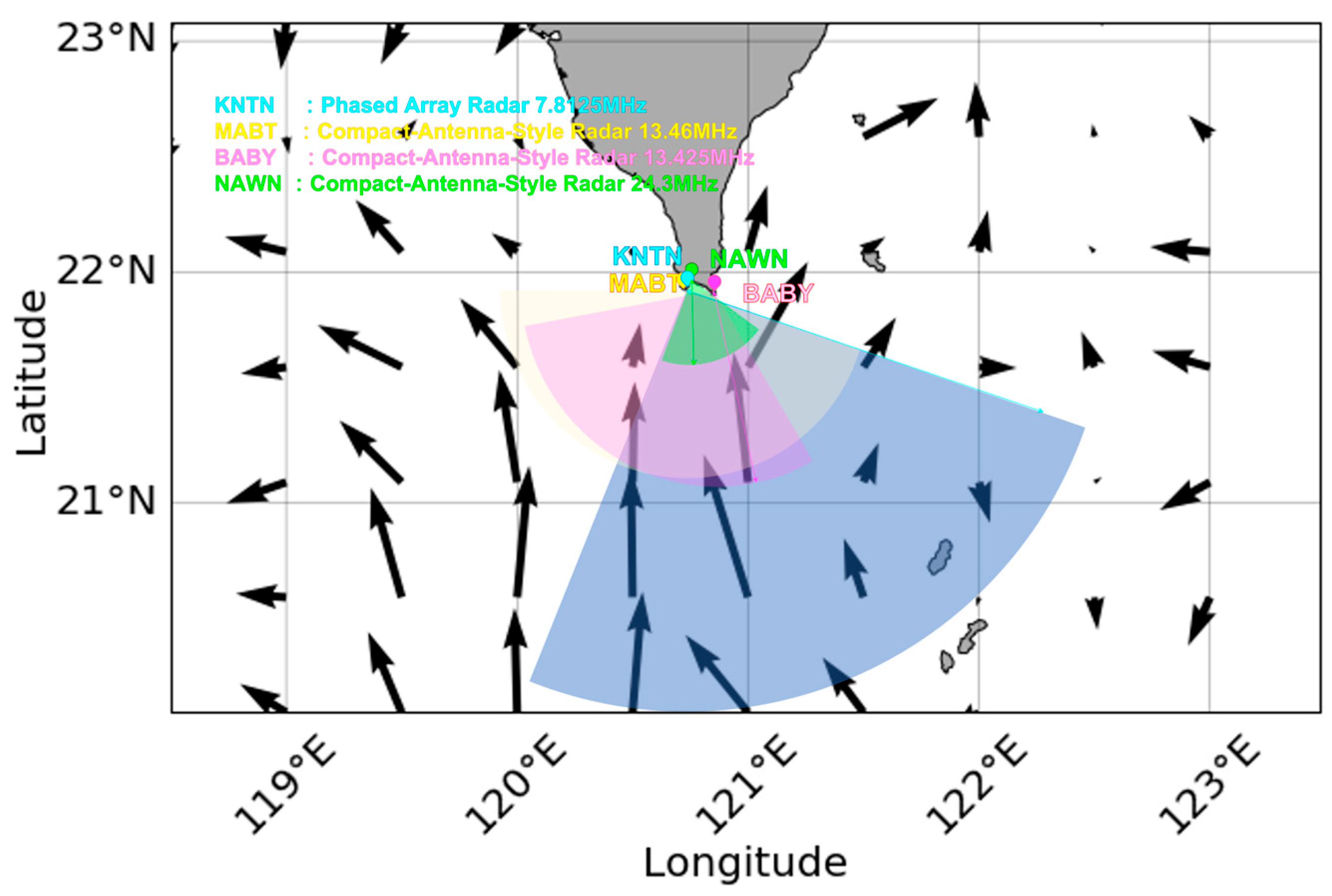
1.3. Overview of the TORI’s Current System at Cape Maobitou

The TORI currently operates three standard CODAR systems and one phased-array LERA system in southern Taiwan. The locations of these radar stations are illustrated in Figure 5, and the key differences between the two systems primarily lie in their antenna configurations. The relevant parameters for each system are listed in

Table 1. High-frequency radar stations in Maobitou.

Parameter	MABT	KNTN
Signal modulation	FMiCW	FMCW linear sweep
Sweep rate	0.5 s	~0.455 s
Central frequency (MHz)	13.425	7.5125
Location	120°44′6.54″ E 21°55′13.20″ N	120°44′6.54″ E 21°55′13.20″ N
Signal modulation	FMiCW	FMCW linear sweep
Sweep rate	0.5 s	~0.455 s

. Radar current measurements determine the direction of arrival (DOA) of target signals through two main methods: array antennas and co-located directional antennas. The former estimate DOA using beamforming (BF), while the latter employ direction-finding (DF) techniques. CODAR systems feature integrated antennas composed of three mutually perpendicular elements. These antennas synchronize to receive signals, record echo energy in voltage values, and use the MUltiple SIgnal Classification (MUSIC) algorithm for DF processing. In contrast, the LERA system at KNTN (Cape Maobitou) utilizes a phased-array antenna configuration to achieve DF.

DF offers a broader observational field of view, potentially up to 360°, but at the expense of angular resolution. BF, on the other hand, uses more complex transmit-and-receive antenna arrays to enhance angular resolution, albeit at higher costs. The accuracy of both systems depends on several factors, including signal-to-noise ratio, geometric configuration, and pointing errors.

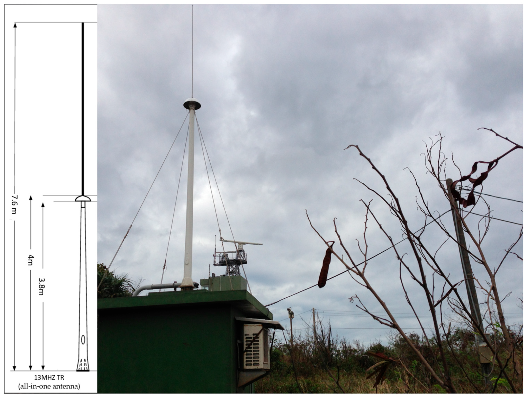
1.3.1. CODAR Systems

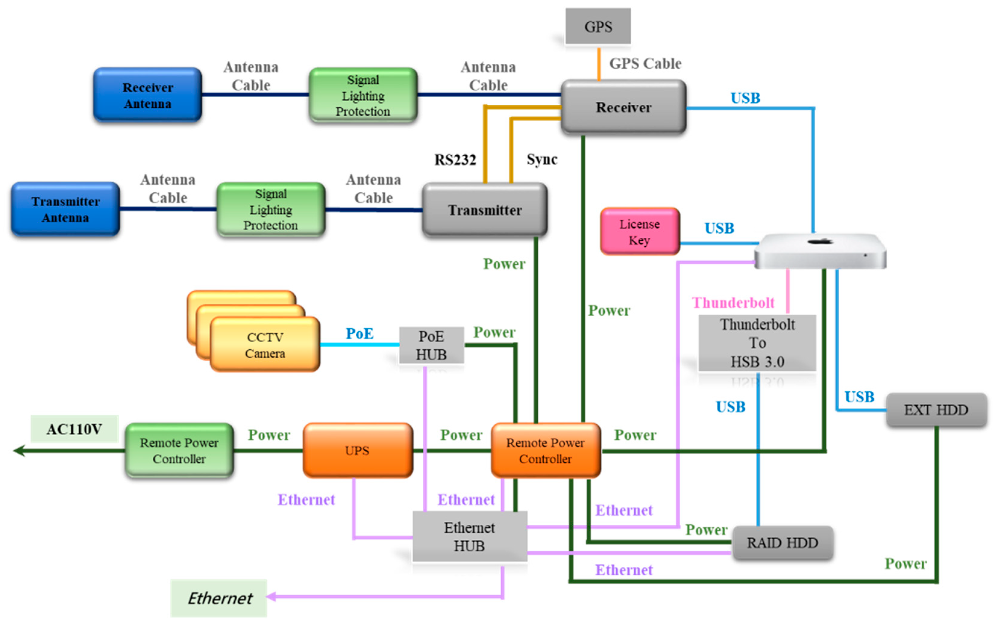
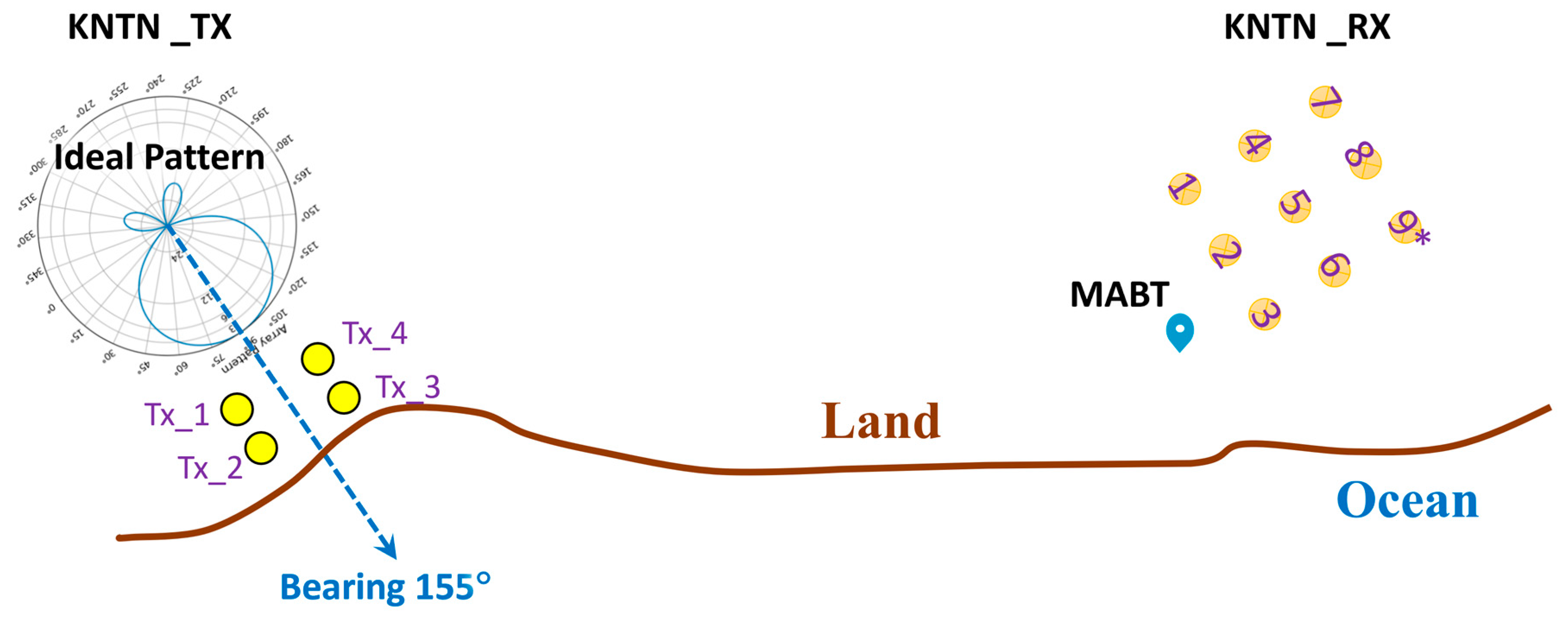
The land-based radar current observation stations at Cape Maobitou, Banana Bay, and Nanwan, implemented by the TORI as part of the TOROS project, employ the CODAR system. The 13 MHz and 24 MHz systems have maximum observation ranges extending approximately 75 km and 40 km offshore, respectively.

The CODAR system transmits omnidirectional radio waves using a 360° transmitting antenna and determines the direction of returned echoes with three mutually perpendicular receiving antennas. Figure 6 depicts the transmitting and receiving antennas at Hengchun station. Unlike conventional shipborne radar, which calculates the distance to an object based on the time difference between transmitted pulses and received echoes, CODAR employs a frequency-modulated interrupted continuous-wave (FMiCW) technique. CODAR’s transmitted radar signals use a chirp pattern (Barrick, 1973 [12]), where the frequency increases or decreases linearly over time. As a result, echoes from different distances correspond to different frequencies, enabling the precise determination of scatterer distances from the radar.

CODAR systems are notable for their high temporal resolution, offering outputs as frequent as every 10 min or as averaged data over one hour or more. However, they exhibit blind spots near the coast (approximately 2 km from shore) due to receiver shutdowns during pulse transmission

1.3.2. LERA (KNTN)

The LERA (Least-Expensive Radar) system, developed by the University of Hawaii, has been deployed in various regions, including the Adriatic Sea, Hawaii, Mexico, and the Philippines. Current operational systems are located in California, the Gulf of Mexico, Hawaii, Quebec, New England, Taiwan, and the Philippines.

The system installed at Cape Maobitou, Hengchun Township, Pingtung County, is an 8 MHz, eight-channel, 3 × 3 phased-array radar system (referred to as KNTN). It includes four transmitting antennas and eight receiving antennas. Unlike CODAR, LERA employs a frequency-modulated continuous-wave (FMCW) approach with a linear chirp transmission period set at 0.455 s and a minimum sampling count of 7600 per chirp. Observations are recorded every 59 min, providing hourly data outputs.

The system is capable of monitoring surface currents within a radius of approximately 250 km and wave characteristics within a range of 100 km. Field tests in Kenting revealed that only 50 kHz of the available frequency range is currently modulated, due to local radiofrequency conditions, resulting in a distance resolution of 3 km per unit.

2. Comparison of Compact (MABT) and Square-Array (KNTN) Ocean Radars

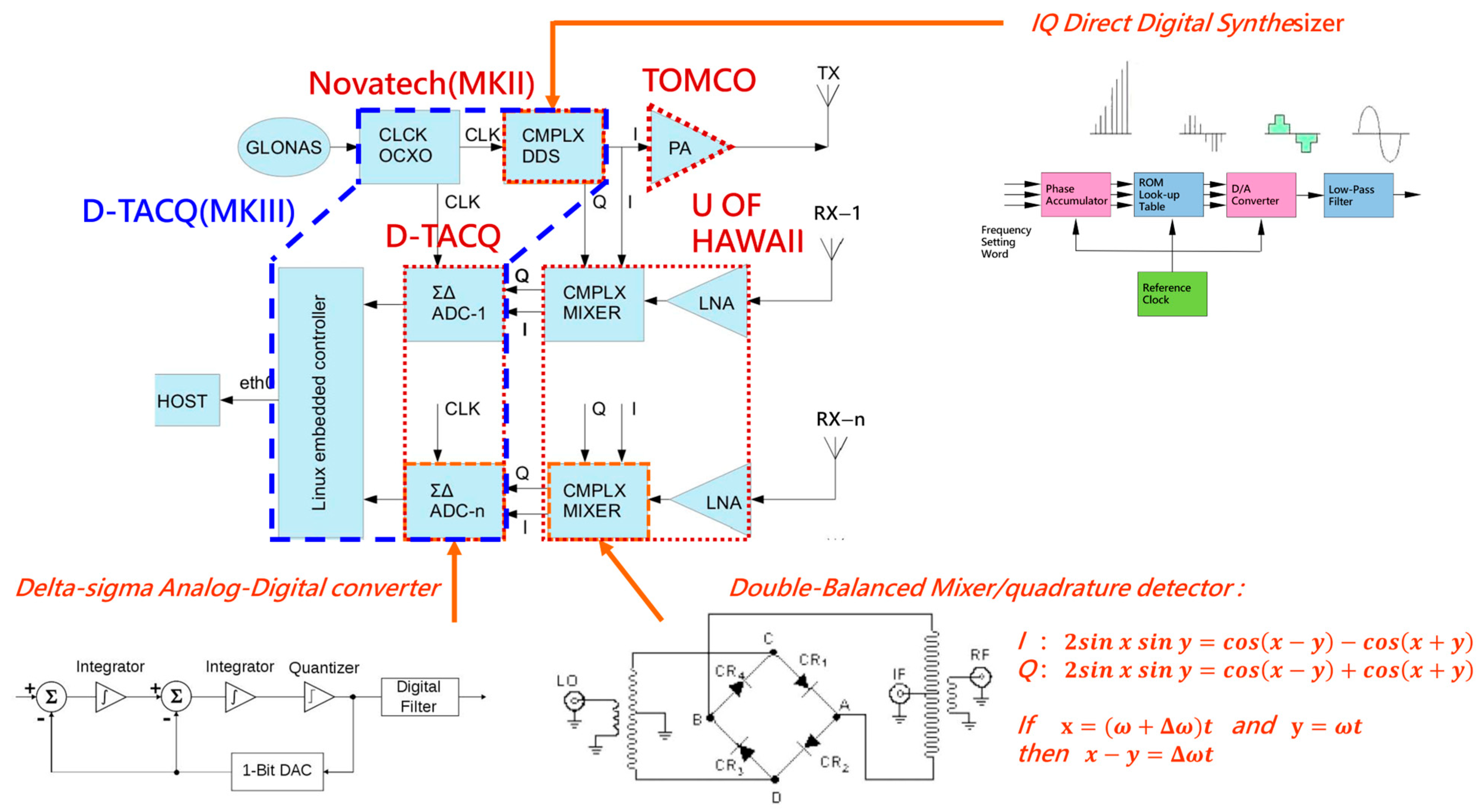
2.1. Hardware Differences

By understanding the key differences in hardware design and algorithm implementation, we can better interpret variations in radar-derived current measurements and their implications for real-time ocean monitoring.

The 13 MHz CODAR system (MABT) at Cape Maobitou was deployed in 2012 by the National Applied Research Laboratories Ocean Center. It employs a combined transmit/receive (TX/RX) antenna and a direction-finding algorithm based on received radar echo intensity (as shown in Figure 6). The system achieves a spatial resolution of 1 km and can measure surface currents within a 70 km radius under optimal conditions. The overall system architecture is shown in Figure 7.

The 8 MHz phased-array radar system (KNTN) at Cape Maobitou, developed by the University of Hawaii, consists of a 3 × 3 antenna array with four transmitting and eight receiving antennas. Unlike CODAR, KNTN employs BF and DF techniques to achieve an angular resolution of less than 2 degrees. The system’s transmission power ranges from 3 to 50 watts, allowing for a monitoring radius of approximately 250 km (as shown in Figure 8).

The hardware components of the KNTN system include a GLONASS satellite timing antenna unit, Direct Digital Synthesis (DDS) function generator, power amplifier (PA), transmitting antenna system (TX), receiving antenna system (RX), sigma-delta analog-to-digital converter (ΔΣ ADC), double-balanced mixer, and Linux-based computer control and analysis unit. The overall system architecture is shown in Figure 9.

The radar waves transmitted by the system are frequency-modulated continuous waves (FMCWs) with linear chirp frequency modulation signals. The operating frequency range is between 3 and 30 MHz, and the transmitted RF power can typically be set between 3 and 5 watts, with a maximum of 50 watts. Signal directional resolution is achieved not only through phase-array BF but also by applying DF techniques, allowing for an azimuthal resolution of less than 2 degrees.

2.2. Algorithm Differences

Although the physical mechanisms of Bragg scattering waves and Doppler frequency shift effects have been clearly defined, real-world ocean observation applications still involve complex signal processing and analysis steps, along with system adjustments based on station environments to improve the accuracy of current observations and the quality of the data.

Ideally, the sea-echo spectra used to analyze surface current speeds should exhibit significant Bragg scattering energy from electromagnetic waves and specific-frequency ocean gravity waves, resulting in first-order peak energy, with second-order peaks surrounding the first due to long-wave energy. However, in real-world ocean environments, electromagnetic backscatter may result in complex, diverse spectra due to varying sea conditions. Therefore, from the perspective of signal processing, the primary task in calculating flow fields from surface feature echoes is to define the range of first-order Bragg echo energy within the spectrum. The SeaSonde high-frequency radar flow measurement system developed by CODAR (CODAR Ocean Sensors, 2002 [13]) provides a signal processing method for setting the first-order peak range, which includes (a) noise threshold setting, (b) smoothing of the spectrum, (c) detection of the boundary between first- and second-order peaks (null point), (d) setting the first-order peak range based on the identified boundary, and (e) using frequency windows to limit the maximum flow speed, among other steps. This process involves five key parameters—noise range, smoothing window size, Doppler spectrum energy range, first-order energy frequency range, and maximum current speed—that must be manually adjusted according to the local station environments and sea conditions (as shown in Figure 10).

The LERA system’s echo information processing allows for flexibility, as it can develop processing procedures based on specific needs. In the KNTN system, the echo direction identification of sea surface signals can utilize beamforming (BF) algorithms that are traditionally used in phased-array systems, but it can also introduce the MUSIC algorithm developed by the Woods Hole Oceanographic Institution (WHOI). This algorithm, proposed by A. Kirincich in 2017 [14], uses radar echo partitioning based on image recognition (as shown in Figure 11 and Figure 12) for first-order peak delineation. The concept is primarily based on watershed partitioning methods in digital image processing, which serve as a tool for partitioning the wave system in the direction spectrum. Using this mechanism can reduce the complexity and subjectivity of traditional first-order peak delineation processes.

To minimize the differences between the two high-frequency radar systems (MABT and KNTN), this study primarily focuses on radial velocity analysis of the adjacent MABT (CODAR) and KNTN (LERA) systems. In terms of sea surface signal echo direction identification, all radial velocity calculations adopt the MUSIC-based algorithm and radar echo segmentation technique using image recognition, aiming to reduce discrepancies between the two systems as much as possible. However, when extracting ocean current information using the MUSIC algorithm, the data preprocessing process involves Doppler analysis of range-resolved time series and Bragg region identification. Laws et al. (2000) [15] pointed out that one of the main sources of error in this technique is the processing of frequency bins outside the Bragg region, meaning that the algorithm incorrectly includes signals that do not belong to the Bragg region in the calculation, leading to erroneous results.

Since low-frequency HF radars have lower velocity resolution, this type of error is particularly significant under low-frequency operational conditions. Therefore, when applying the MUSIC algorithm, careful Bragg region identification is essential to minimize calculation errors and improve the accuracy of ocean current measurements.

In addition to differences in radar configurations and signal processing approaches, existing research has provided comparative assessments between different types of HF radar systems and their correspondence with in situ measurements. For instance, Liu et al. (2018) [16] conducted a side-by-side comparison of long-range CODAR SeaSonde and medium-range WERA radar systems deployed at the same site on the West Florida Shelf. Their study demonstrated significant spatial and temporal variability in data return performance between the two systems, as well as systematic differences in velocity accuracy when compared against moored ADCP data. CODAR tended to perform better under high-sea-state conditions during daytime, whereas WERA showed relatively consistent performance with some advantages at night, highlighting the importance of frequency selection and the local environment in radar deployment.

Additionally, Rayner (2010) [17] emphasized the operational importance of integrated ocean observation systems such as the U.S. IOOS, as well as how data collected from multiple HF radar networks must be properly standardized and harmonized to ensure interoperability. These studies form a critical foundation for evaluating system-specific performance, integration feasibility, and radar data consistency. Building on this prior work, the present study focuses on the comparative evaluation of two technically distinct HF radar systems located in adjacent areas in southern Taiwan, processed through a unified quality control framework and validated against surface drifter observations.

3. Methodology

Accurate radial velocity is crucial for improving the precision and resolution of the synthesized flow field. However, when combining radial data from multiple radar systems, inconsistencies in data quality and system characteristics can reduce the reliability of the merged vector field. As highlighted in Section 2.2, previous studies (e.g., Liu et al., 2018 [16]; Rayner, 2010 [17]) have shown that different HF radar systems may perform differently under varying conditions, due to differences in antenna design, frequency, and signal processing parameters. To support future multi-system integration and ensure comparability, it is essential to evaluate the performance of individual radar systems through cross-validation with in situ observations. Therefore, this study focuses on the radial velocity derived from two HF radar systems of different configurations deployed in adjacent areas, processed using a unified methodology. The goal is to assess the accuracy, consistency, and potential for integration, especially in overlapping observational domains.

High-frequency ocean radar utilizes the Bragg resonance effect between electromagnetic waves and ocean surface gravity waves, which generates backscatter. As described in Section 1.1, this Bragg scattering mechanism results in a strong reflected radar signal. A typical reflected spectrum is shown in Figure 13, which is primarily provided by the moving waves on the ocean surface and contains a wealth of oceanic information (such as currents, winds, wave fields, etc.), as well as other environmental data.

This study focuses on the first-order Bragg peaks in the backscattered spectrum, as these signals are generated through resonance with surface gravity waves, and their Doppler shift is directly related to the radial component of surface current velocity. Based on the theoretical framework proposed by Barrick (1972) [9,10], the use of first-order peaks has become a standard practice in operational HF radar systems worldwide for current retrieval. Accordingly, this study follows this established methodological framework. By analyzing the received echo signal and the Doppler shift caused by the surface current relative to the emitted frequency, we can estimate the radial ocean current velocity (the flow velocity component in the direction of the radar antenna). By defining the first-order Bragg peak range and employing the Doppler frequency shift principle, the radial velocity associated with surface gravity waves can be quantitatively estimated. After compiling the results from all of the measurement points, we can obtain the radial ocean current data (radial velocity file, RUV file) for each point in the circular annulus surrounding the radar station, with a fixed distance separation.

A single high-frequency radar can only measure ocean current information along the radial direction of the antenna, providing data about the flow moving away from or toward the radar. However, since flow velocity is a vector, it must be represented by two orthogonal components. Therefore, it is necessary to combine data from dual or multiple high-frequency radar systems to express the two-dimensional flow field within the overlapping region covered by the radars. If there are inconsistencies or unreasonable differences in the quality of the radial velocity, it may reduce the accuracy of the synthesized results.

Moreover, high-quality radial velocity helps preserve the features of the observed flow field, significantly impacting whether the synthesized flow field can effectively capture local variations in the flow. In simple terms, high-quality radial velocity is a key factor in ensuring the accuracy and reliability of the subsequent synthesized flow field. The following analysis will focus on the discussion of the physical quantities of radial velocity.

3.1. Methods for Reducing the Impact of Analytical Differences

The radar wave echo signal is received by the system and recorded as complex I (in-phase) and Q (quadrature-phase) data. The I/Q function is used to obtain information such as echo strength and phase. By integrating the real part (I-voltage) and imaginary part (Q-voltage) into a complex echo time series, the first Fast Fourier Transform (FFT) is performed to analyze the echo time series, obtaining the distance sequence. A second FFT is then applied to derive the Doppler distance spectrum (as shown in Figure 13). In the Doppler distance spectrum, positive and negative frequency values represent the direction of movement of the observed Bragg waves, with positive indicating toward the radar and negative indicating away from the radar. The calculation process for radial velocity in the Doppler distance spectrum for the MABT (CODAR) and KNTN (LERA) systems is shown in Figure 14.

In terms of spatial resolution, the distance between the two sites is only 0.9 km, and the radial grid points for both stations show minimal differences in bearing (approximately a few degrees). The distance resolution is influenced by the bandwidth, with KNTN having a bandwidth of 50 KHz and MABT 100 KHz, corresponding to distance resolutions of 3 km and 1.5 km, respectively (Figure 15 and Figure 16). Therefore, a 5-degree averaging result is applied for angle resolution, and for distance resolution, KNTN uses a range of ±1 radar cell (RC) and MABT uses ±2 RC to minimize the spatial differences between the two systems.

In terms of temporal resolution, both systems use hourly data. KNTN primarily observes the data from the 59 min preceding each hour, representing data for the full hour. MABT, based on the original settings, splits the data around the hour into two halves, before and after the hour. For example, at 06:00, KNTN represents data from 05:00 to 05:59, while MABT represents data from 05:30 to 06:30. To standardize the temporal resolution between the two systems, this study adjusted the MABT file names to 05:30 to represent 06:00, addressing the time resolution differences between the two systems (Figure 17).

3.2. Using Drifting Buoys and Data Buoys for Current Measurement to Validate Two Radar-Based Current Measurement Systems

HF radar determines ocean surface currents by extracting the first-order Bragg peak frequency shift from the Doppler spectrum and applying beamforming and MUSIC DF methods to infer radial velocity. The radial velocity for each range cell is sequentially solved to construct the overall ocean surface current field. However, even under optimal operating conditions, the coverage area of HF radar is influenced by factors such as the height of Bragg resonant waves, sea surface propagation loss, background noise levels, and the intensity of interfering signals. In the case of MUSIC processing, a limited signal-to-noise ratio (SNR), antenna pattern effects, or the intrinsic characteristics of ocean currents may result in sparse or incomplete coverage. In other words, HF radar current measurement is not a system that can consistently provide stable observations across all ranges and angular domains. For instance, if the radial component of the current remains nearly uniform over a wide angular sector within a given range cell, the MUSIC algorithm may yield only a few angle solutions, leading to apparent gaps in coverage.

To verify the reliability of HF radar-derived current measurements, this study compares the radial velocities derived from KNTN and MABT with trajectory data from the GDP. This comparison aims to assess the accuracy and consistency of the two radar systems when applied to the same oceanic region.

Before data comparison, data matching is a critical prerequisite and one of the most challenging aspects of quantitative validation. Since HF radar and drifter measurements are based on the Eulerian and Lagrangian coordinate systems, respectively, appropriate data analysis techniques are required for meaningful comparison. In this study, the coefficient of correlation and RMSD are adopted as quantitative metrics to evaluate the consistency and discrepancies between HF radar-derived currents and drifter observations.

4. Results and Discussion

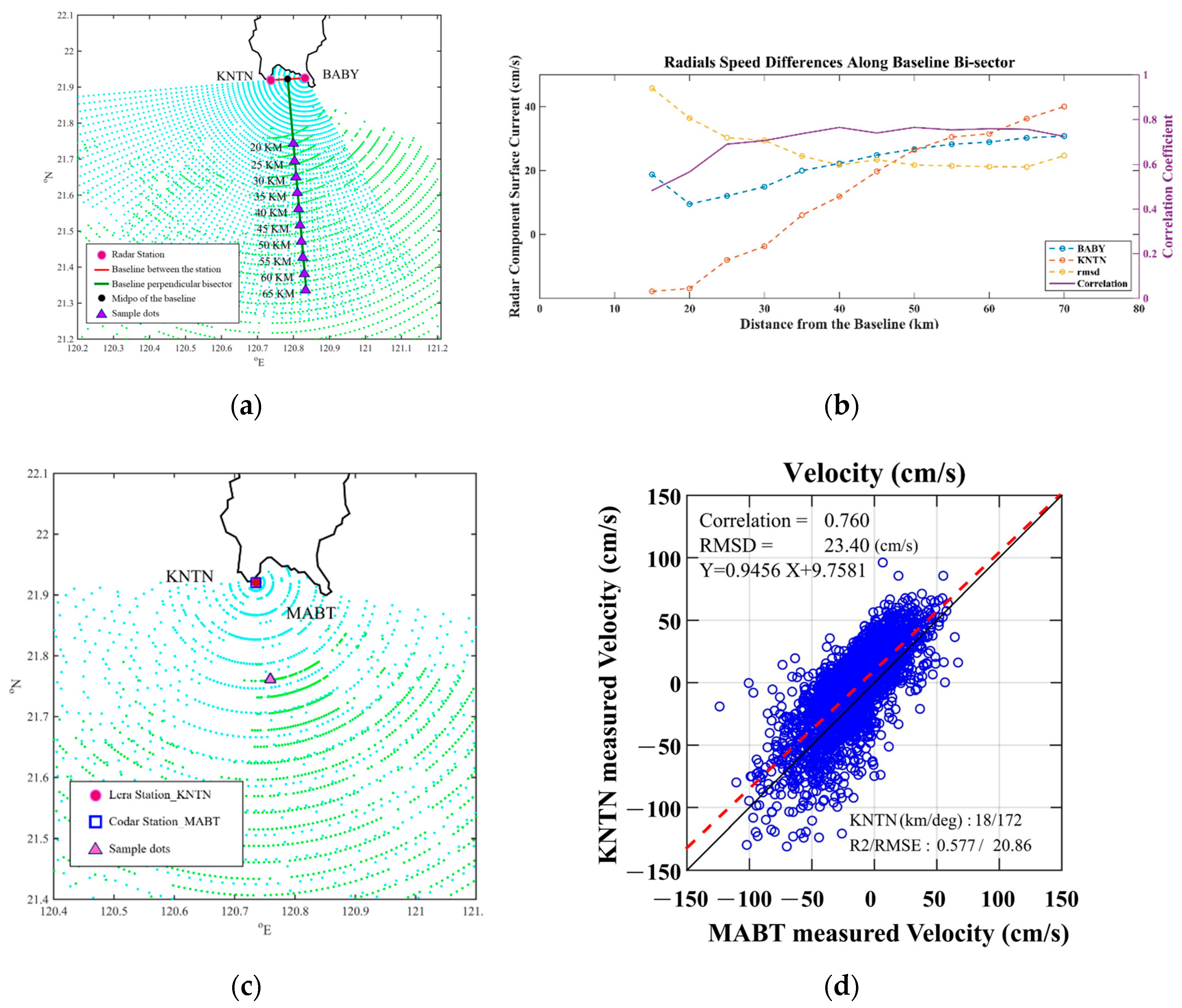
4.1. Differences in Radial Velocity (Baseline Velocity Comparisons)

HF ocean radars offer advantages such as long-range coverage, wide spatial extent, and cost-effectiveness, making them widely used for ocean current observations in recent years. However, the validation of radar-derived current measurements has traditionally relied on single-point Acoustic Doppler Current Profiler (ADCP) observations or a limited number of drifting buoys, both of which require significant time and financial investment. Furthermore, discrepancies between moored buoys and radar-derived currents arise from several factors. In addition to the inherent differences in measurement methods—moored buoys provide single-point intrusive measurements, while radar systems operate via remote sensing—nearshore deployments are particularly affected by complex coastal topography, which can reduce the spatial homogeneity of ocean currents, thereby impacting the correlation between the two measurement systems.

To assess the uncertainty of velocity measurements in HF radar systems, Paduan et al. (2006) [18] proposed the baseline velocity comparisons method, which provides a rapid and continuous means of evaluating radar-derived current velocities by ensuring that the spatial and temporal scales of the measurements are properly matched. Ideally, baseline velocity comparisons involve two independent radar stations, with their velocity measurements compared at the midpoint along the baseline connecting them.

In the southern waters of Taiwan, three integrated HF radar stations operate in addition to the phased-array radar station KNTN. This study employs baseline velocity comparisons to evaluate the performance of these three operational radar systems (

Table 2. High-frequency radar stations in southwestern Taiwan.

	MABT	NAWN	BABY	KNTN
Central frequency (MHz)	13.425	24.3	13.40	7.8125
Location	120°44′6.54″ E 21°55′13.20″ N	120°45′41.46″ E 21°57′34.32″ N	120°49′50.46″ E 21°55′34.02″ N	120°44′6.54″ E 21°55′13.20″ N
Bandwidth (KHz)	100	100	100	50
Range resolution (km)	1.5	0.7	1.5	3
RXx antenna type	$\lambda /8$-length active non-resonant monopoles	Compact type	Compact type	Compact type

). Among them, the MABT can be directly compared with KNTN along a shared baseline. However, the ideal baseline between KNTN and the Banana Bay (BABY) station falls within a blind zone of KNTN. Therefore, we adopted the baseline comparison approach proposed by Atwater and Heron (2010) [19], selecting measurement points along the perpendicular bisector of the baseline at intervals of 10 km between 20 km and 60 km to compare the radial velocities.

The comparison between KNTN and MABT from June to December 2022 revealed a correlation coefficient of approximately 0.77 (Figure 18), with an RMSD of 0.23 m/s. The observed differences in radial velocity accuracy between KNTN and MABT could be attributed to their respective antenna configurations and signal processing techniques. While KNTN’s broader coverage enhances spatial observations, potential edge effects may introduce additional measurement uncertainties. Conversely, MABT’s lower frequency band improves nearshore precision but may have reduced long-range detection capabilities. According to Jeffrey D. et al. (2006) [18], baseline velocity comparisons typically yield correlation coefficients between 0.60 and 0.81, with the RMSD values ranging from 0.12 to 0.13 m/s. Similarly, Dao et al. (2019) [20] reported that the comparison between the phased-array radar system HTCN in Taichung Harbor and the nearby CODAR system TUTL produced correlation coefficients between 0.76 and 0.82, with RMSD values between 0.06 and 0.12 m/s, consistent with our findings.

Regarding the comparison between KNTN and BABY along the perpendicular bisector of their baseline, the results are shown in Figure 18c,d. The data indicate that as the observation points move farther from the baseline’s midpoint, the RMSD of the radial velocity measurements gradually decreases. At approximately 40 km from the baseline’s midpoint, the RMSD stabilizes around 20 cm/s, while the correlation coefficient of radial velocities between the two radar stations remains above 0.7. In the nearshore region (15–30 km), the RMSD ranges from 29.5 to 36.5 cm/s, with correlation coefficients between 0.57 and 0.71.

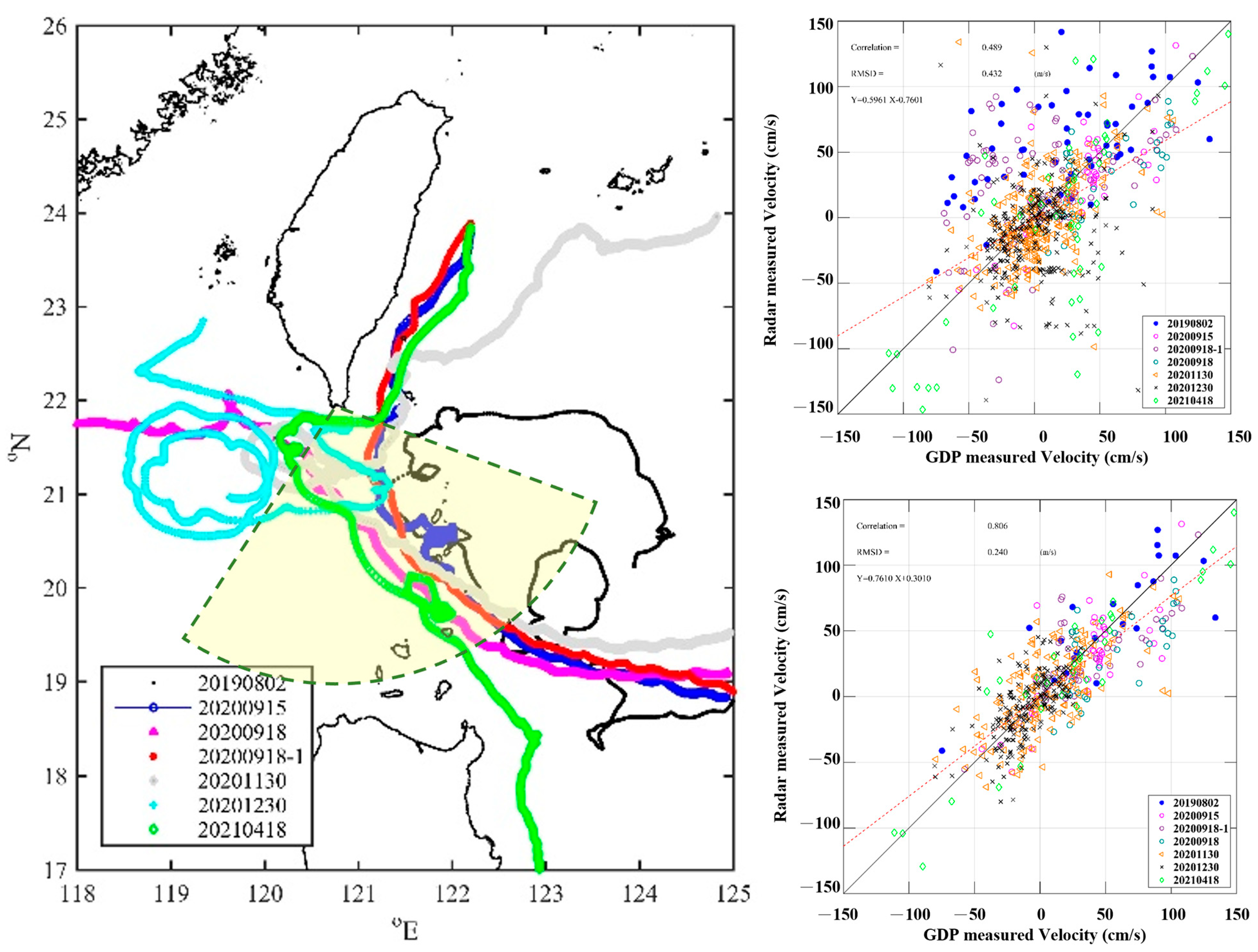
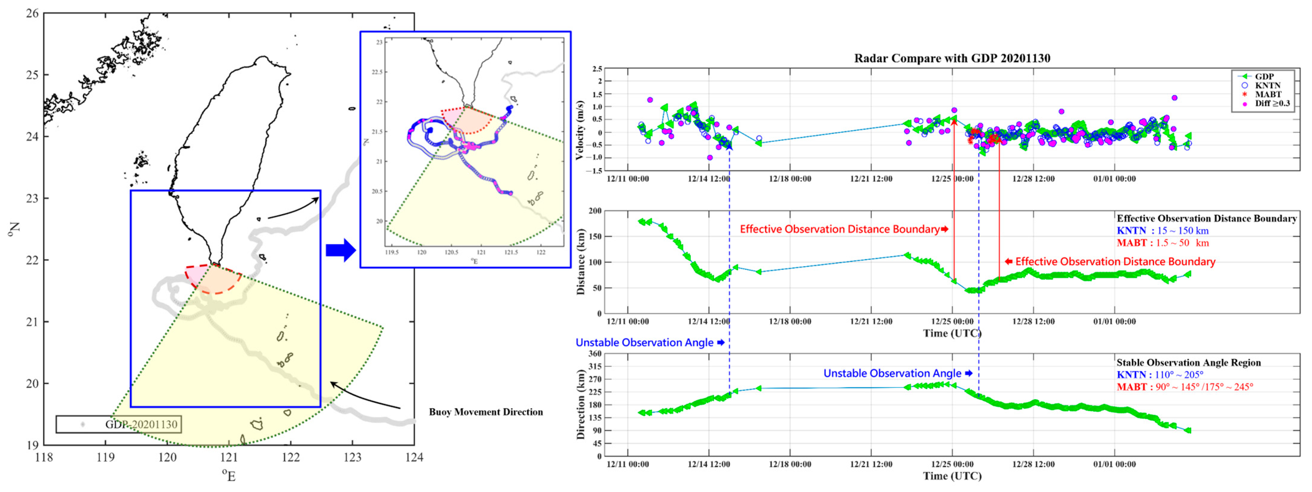
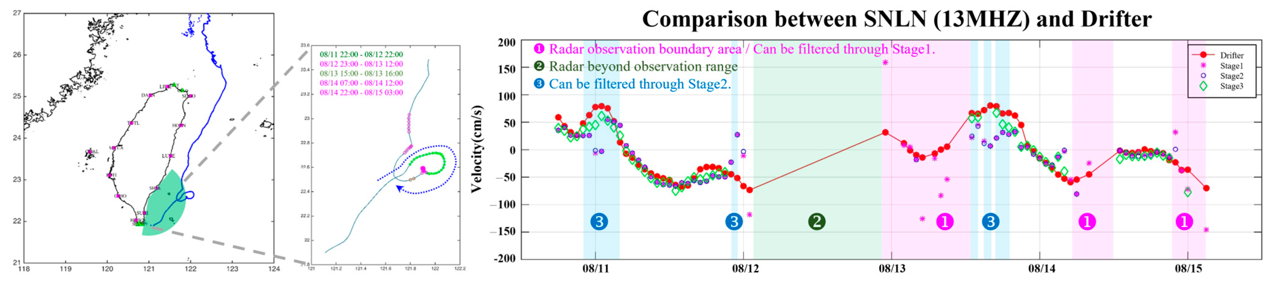
4.2. Drifter-Based Velocity Comparisons

From April 2019 to December 2021, the trajectories of GDP surface drifters were analyzed to evaluate the reliability of radar-derived radial velocity measurements.

During the operation of KNTN, a total of seven GDP drifters passed through its observation area, with their trajectories shown in Figure 19. Overall, the comparison between KNTN-measured radial velocity and GDP drifter observations yielded an average correlation coefficient of 0.49 and an RMSD of 0.43 m/s. When focusing solely on regions with stable data availability, defined as areas where the radar radial velocity output rate exceeded 70%, the average correlation increased to 0.81, while the RMSD decreased to 0.24 m/s, indicating a higher consistency between radar-derived and drifter-observed velocity data in stable environments.

Furthermore, only two GDP drifters (GDP-20201130 and GDP-20201220) simultaneously passed through the MABT and KNTN observation areas while both radar systems were operating normally. The comparison results show that, for KNTN, the correlation coefficients were 0.48 and 0.51, with RMSD values of 0.32 m/s and 0.23 m/s, respectively (Figure 20). For MABT, the correlation coefficients were 0.64 and 0.64, with RMSD values of 0.32 m/s and 0.22 m/s, respectively (Figure 21). In Figure 20 and Figure 21, the red and yellow sectors represent the observation ranges of the MABT and KNTN stations, respectively. The blue lines with circles indicate the drifter trajectories, while the magenta circles mark locations where the velocity difference exceeds 0.3 m/s.

By applying the QC process developed by the TORI, the correlation of KNTN improved to 0.58 and 0.65, while the RMSD decreased to 0.24 m/s and 0.17 m/s (Figure 22). This QC mechanism was developed based on the QARTOD manual (U.S. IOOS—Integrated Ocean Observing System, 2016) [4], integrating team expertise to establish a quality control procedure tailored for HF radar-derived current measurements, enhancing the data’s reliability and consistency. The newly developed QC mechanism consists of three major procedures (Figure 23):

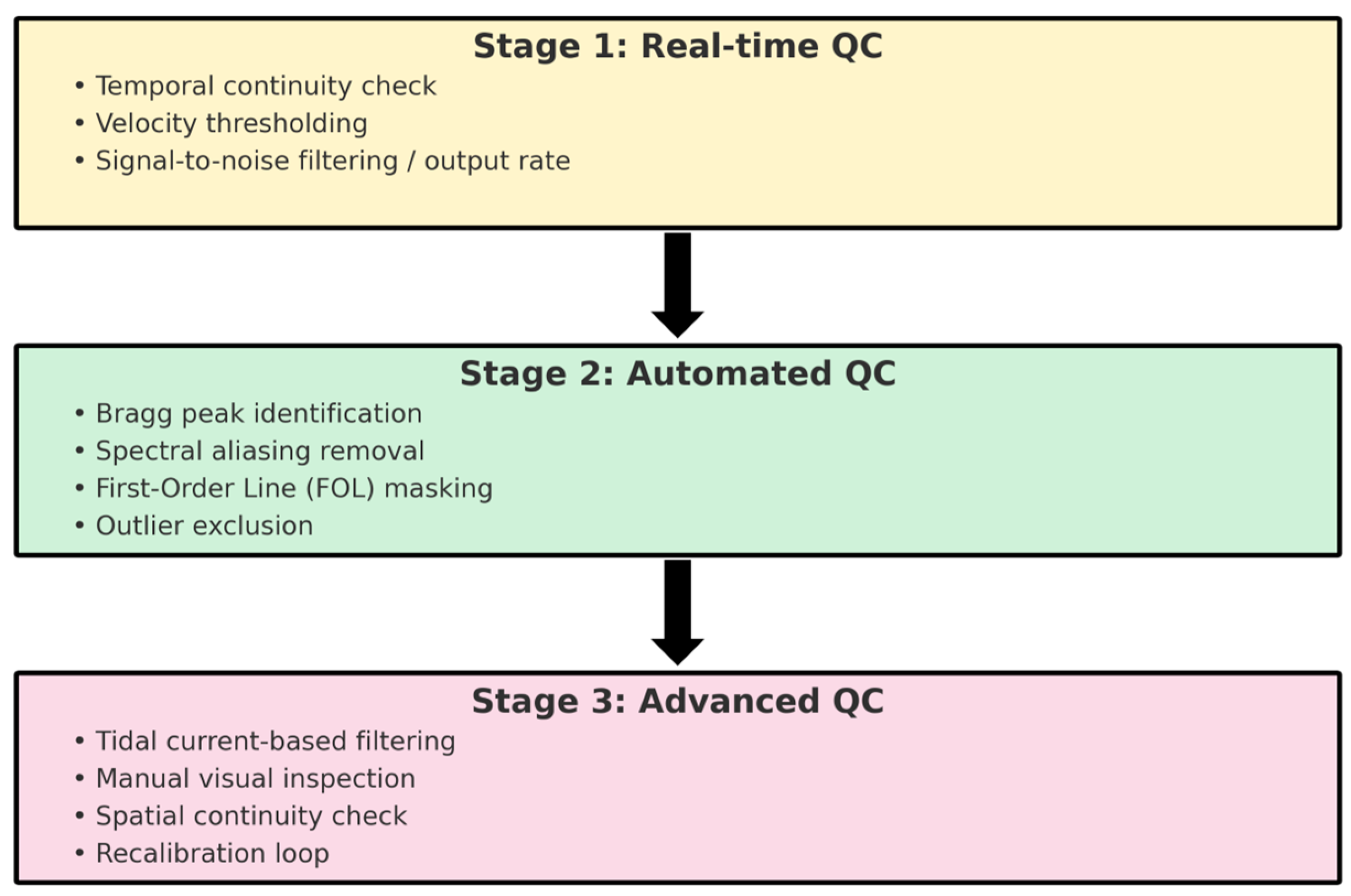
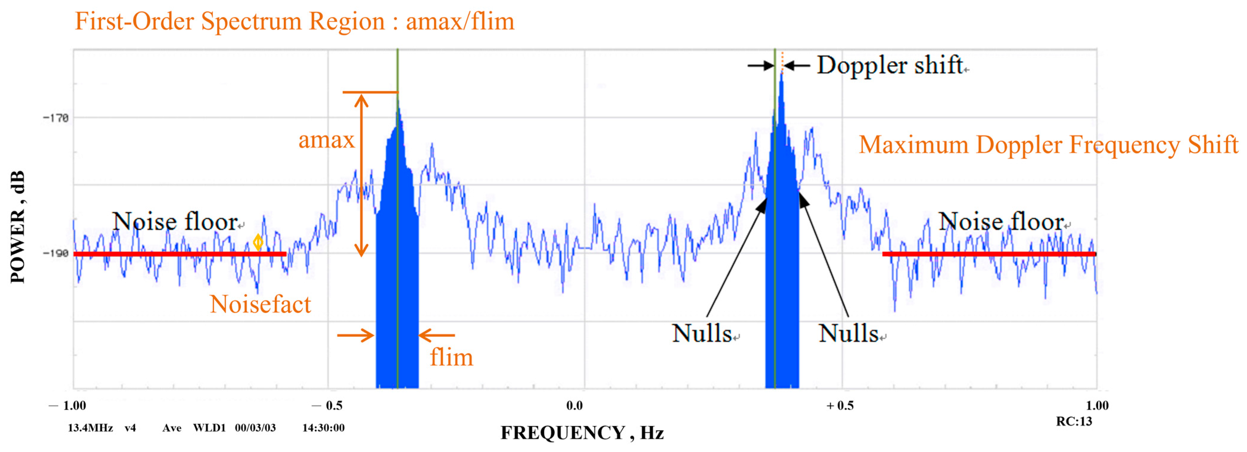
• Data Integrity Verification: This step examines the file headers, footers, and overall data format and content to eliminate errors caused by radar system hardware malfunctions or analytical software anomalies. Additionally, spectral analysis and harmonic analysis are used to assess whether the radar-measured currents conform to the historical tidal characteristics of the observation area and whether the obtained current data follow a normal distribution.
• Data Validity Assessment: Based on the sampling theorem, the effective data production rate for each grid point is calculated to ensure that the produced data accurately reflect tidal variations.
• Anomalous Data Filtering: The mean and standard deviation of the measured current data are analyzed to detect excessively high or low values, ensuring temporal and spatial continuity and reasonability of the dataset.

Figure 22. Time series of radial velocity for KNTN with and without quality control compared to GDP-20201220.

Figure 22. Time series of radial velocity for KNTN with and without quality control compared to GDP-20201220.

Figure 23. Three-stage quality control (QC) process for high-frequency radar radial current data along the coast of Taiwan.

Figure 23. Three-stage quality control (QC) process for high-frequency radar radial current data along the coast of Taiwan.

Figure 24 presents the radar-derived radial current data processed through three quality control (QC) stages and their comparisons with in situ measurements from surface drifters. The results indicate a progressive improvement in data quality across the stages. In Stage 1 (real-time QC), the correlation coefficient was 0.68, with a root-mean-square deviation (RMSD) of 38.36 cm/s. After applying the automated QC in Stage 2, the correlation increased to 0.78 and the RMSD decreased to 30.69 cm/s. Finally, with the implementation of advanced QC procedures in Stage 3, the correlation reached 0.96 and the RMSD was further reduced to 15.24 cm/s. These findings confirm that the multi-stage QC framework developed in this study significantly improves the stability, reliability, and consistency of HF radar surface current observations.

Since the trajectory of GDP-20201130 was near the boundary of MABT’s observation range, there were insufficient data points for comparison after quality control. Meanwhile, the correlation between GDP-20201220 and MABT improved to 0.78, with the RMSE reduced to 0.16 m/s (Figure 25). These results demonstrate that a systematic QC mechanism effectively eliminates anomalous data, enhancing the accuracy and reliability of HF radar-derived current measurements.

According to Kirincich et al. (2019) [21], a study from the Woods Hole Oceanographic Institution (WHOI) on the comparison between phased-array radar-derived currents and drifter observations indicated that, with the Peak Thresh setting, the overall correlation was approximately 0.59, with an RMSD of 0.18 m/s. In stable regions, the correlation increased to 0.74, with an RMSD of 0.14 m/s. Based on this comparison, this study concludes that the KNTN radar-derived velocity measurements are of moderate quality relative to drifter observations.

4.3. Differences and Influencing Factors in Surface Current Measurements Between Compact and Phased-Array HF Radars and Drifters

HF radars estimate sea surface radial velocity based on Doppler frequency shifts, which inherently involve spatial and temporal averaging effects. However, the results from the GDP surface drifter trajectories indicate that the flow structure in the southern waters of Taiwan is highly complex. If the spatial and temporal averaging scale is too large, small-scale current variations may be lost; conversely, if the scale is too small, increased data fluctuations may affect computational accuracy, thereby reducing the reliability of the current measurements.

In terms of hardware configuration, the MABT system adopts an integrated radar architecture with only three receiving antennas, whereas the KNTN system is a phased-array radar with eight receiving antennas. The differences in the number and arrangement of the antennas may impact the direction-finding accuracy and data completeness.

Additionally, system parameter settings also influence radar-derived current measurements. MABT and KNTN differ not only in their receiving antenna configurations but also in their central frequency and bandwidth settings. These technical differences affect the observational range and resolution of the estimated radial velocity, thereby influencing the measurement accuracy and consistency. Since MABT and KNTN operate at different frequency bands, inherent differences exist in their velocity resolution, observation range, and applicable water depths. Furthermore, different frequency bands exhibit varying sensitivities to environmental interference, which may further impact the stability and accuracy of the radar current measurements.

Therefore, when comparing results from different radar systems, it is essential to comprehensively consider the effects of the observation environment, hardware architecture, and system parameter settings to ensure the accuracy and reliability of the analysis.

5. Conclusions

This study presents a site-specific comparative analysis of two coastal HF radar systems deployed in Taiwan: the 13 MHz CODAR system, and the 8 MHz phased-array radar system. Using data from the GDP as a reference, we evaluated the measurement accuracy, spatial coverage, and radar applicability under comparable environmental conditions. The results show that the phased-array system offers broader spatial coverage, while the CODAR system exhibits superior nearshore accuracy. Both systems demonstrate robust performance within their respective operational domains.

A three-stage QC mechanism was developed and implemented to improve the consistency and reliability of radar-derived current measurements. Validation against drifter data showed that the QC process significantly enhances correlation and reduces the RMSD by filtering out temporal and spatial anomalies.

To support long-term multi-system integration in Taiwan’s coastal HF radar network, this study contributes in four major ways:

• It introduces a locally adapted QC framework designed from empirical operational experience to improve the consistency of radial velocity observations.
• It constructs a rare synchronous dataset from two different HF radar systems operating over the same time and space, with independent validation from drifter observations.
• It examines the effects of operating frequency differences (8 MHz vs. 13 MHz) on data quality and spatial resolution, providing practical insights for multi-frequency data fusion and model assimilation.
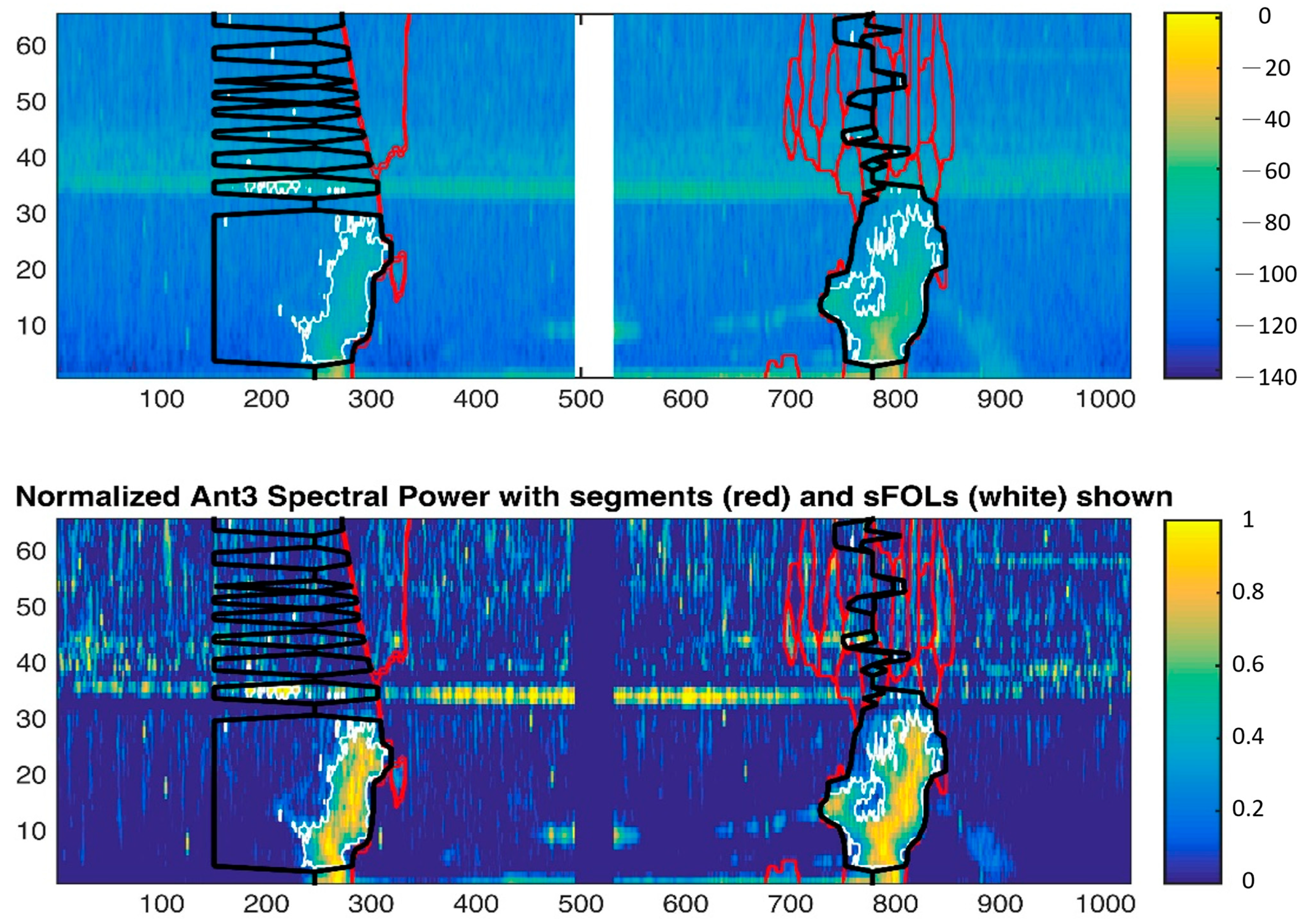
• It applies a unified Bragg peak identification algorithm (MUSIC) across both systems, thereby evaluating its performance and consistency across heterogeneous radar platforms.

Rather than emphasizing performance superiority between systems, this study focused on minimizing system-based discrepancies under real-world observational constraints, offering practical methods for cross-validation, and outlining pathways for integration. The findings are intended to inform the future development of error harmonization protocols, multi-system calibration, and coupled ocean–atmosphere model assimilation strategies.

While this study did not explicitly focus on atmospheric influences, we acknowledge that ionospheric disturbances, especially during nighttime or periods of strong solar activity, can affect HF radar signal quality. Future research will investigate such impacts using spectral separation methods, such as cross-spectral analysis, to enhance data stability under varying environmental conditions. These efforts will further support the long-term development of multi-frequency integrated radar networks and real-time coastal current monitoring in dynamically complex regions like Taiwan.

References

1. Crombie, D.D. Doppler spectrum of sea echo at 13.56 Mc./s. Nature 1955, 175, 681–682. [Google Scholar] [CrossRef]
2. Barrick, D. First-order theory and analysis of mf/hf/vhf scatter from the sea. IEEE Trans. Antennas Propag. 1972, AP-20, 2–10. [Google Scholar] [CrossRef]
3. Barrick, D. Remote sensing of sea state by radar. In Proceedings of the Ocean 72—IEEE International Conference on Engineering in the Ocean Environment, Newport, RI, USA, 13–15 September 1972; pp. 186–192. [Google Scholar]
4. Roarty, H.; Cook, T.; Hazard, L.; George, D.; Harlan, J.; Cosoli, S.; Grilli, S. The global high-frequency radar network. Front. Mar. Sci. 2019, 6, 164. [Google Scholar] [CrossRef]
5. Barrick, D.E.; Evans, M.W.; Weber, B.L. Ocean surface currents mapped by radar. Science 1977, 198, 138–144. [Google Scholar] [CrossRef] [PubMed]
6. Wang, C.Y.; Su, C.L.; Wu, K.H.; Chu, Y.H. Cross spectral analysis of CODAR-SeaSonde echoes from sea surface and ionosphere at Taiwan. Int. J. Antennas Propag. 2017, 2017, 756761. [Google Scholar] [CrossRef]
7. Roarty, H.; Smith, M.; Evans, C.; Handel, E.; Kohut, J.; Glenn, S. Quality control for a network of SeaSonde HF radars. In Proceedings of the IEEE OCEANS 2014, Taipei, Taiwan, 7–10 April 2014. [Google Scholar]
8. Haines, S.; Seim, H.; Muglia, M. Implementing quality control of high-frequency radar estimates and application to Gulf Stream surface currents. J. Atmos. Ocean. Technol. 2017, 34, 1207–1224. [Google Scholar] [CrossRef]
9. U.S. IOOS—Integrated Ocean Observing System. Manual for Real-Time Quality Control of High-Frequency Radar Surface Currents Data: A Guide to Quality Control and Quality Assurance of High-Frequency Radar Surface Currents Data Observations, Version 2.0; U.S. IOOS—Integrated Ocean Observing System: Maryland, MD, USA, 2016. [Google Scholar]
10. Lai, J.-W.; Wu, C.-C.; Huang, Y.-H.; Chen, S.-H. A Proposal and evaluation of data QA/QC processes for Taiwan Ocean Radar Observing System. In Proceedings of the 18th Pacific-Asian Marginal Seas Meeting (PAMS), Okinawa, Japan, 21–23 April 2015. [Google Scholar]
11. Kirincich, A.R.; de Paolo, T.; Terrill, E. Improving HF radar estimates of surface currents using signal quality metrics, with application to the MVCO high-resolution radar system. J. Atmos. Ocean. Technol. 2012, 29, 1377–1390. [Google Scholar] [CrossRef]
12. Barrick, D.E. FM/CW Radar Signals and Digital Processing; NOAA-TR-ERL-283-WPL-26; National Oceanic and Atmospheric Administration: Boulder, CO, USA, 1973. [Google Scholar]
13. Barrick, D.E. First-Order Region Boundaries; Technical Report; CODAR Ocean Sensors Ltd.: Mountain View, CA, USA, 2002; p. 9. [Google Scholar]
14. Kirincich, A.R. Improved detection of the first-order region for direction-finding HF radars using image processing techniques. J. Atmos. Ocean. Technol. 2017, 34, 1679–1691. [Google Scholar] [CrossRef]
15. Laws, K.E.; Fernandez, D.M.; Paduan, J.D. Simulation-based evaluations of HF radar ocean current algorithms. IEEE J. Ocean. Eng. 2000, 25, 481–491. [Google Scholar] [CrossRef]
16. Liu, Y.; Merz, C.R.; Weisberg, R.H.; O’Loughlin, B.K.; Subramanian, V. Data return aspects of CODAR and WERA high-frequency radars in mapping currents. In Observing the Oceans in Real Time; Venkatesan, R., Tandon, A., D’Asaro, E., Atmanand, M.A., Eds.; Springer: Berlin/Heidelberg, Germany, 2017; pp. 227–239. [Google Scholar] [CrossRef]
17. Rayner, R. The U.S. integrated ocean observing system in a global context. Mar. Technol. Soc. J. 2010, 44, 26–31. [Google Scholar] [CrossRef]
18. Paduan, J.D.; Kim, K.; Cook, M.; Chavez, F. Calibration and validation of direction-finding high-frequency radar ocean surface current observations. IEEE J. Ocean. Eng. 2006, 31, 862–875. [Google Scholar] [CrossRef]
19. Atwater, D.P.; Heron, M.L. HF radar two-station baseline bisector comparisons of radial components. In Proceedings of the IEEE Oceans 2010, Sydney, Australia, 24–27 May 2010; pp. 1–4. [Google Scholar]
20. Dao, D.T.; Chien, H.; Lai, J.W.; Huang, Y.H.; Flament, P. Evaluation of HF radar in mapping surface wave field in Taiwan Strait under winter monsoon. In Proceedings of the OCEANS 2019, Marseille, France, 17–20 June 2019; Institute of Electrical and Electronics Engineers Inc.: New Jersey, NJ, USA, 2019. [Google Scholar] [CrossRef]
21. Kirincich, A.; Emery, B.; Washburn, L.; Flament, P. Improving surface current resolution using direction-finding algorithms for multiantenna high-frequency radars. J. Atmos. Ocean. Technol. 2019, 36, 1997–2014. [Google Scholar] [CrossRef]
Figure 4. Schematic map of high-frequency ocean radar distribution in Taiwan, including CODAR and phased-array radar deployments at key observation stations.
Jmse 13 00778 g004
Figure 5. Schematic map of radar station locations in southern Taiwan established by the ocean.
Jmse 13 00778 g005
Figure 6. Maobitou 13 MHz CODAR all-in-one antenna diagram.
Jmse 13 00778 g006
Figure 7. Maobitou 13 MHz CODAR radar architecture diagram (revised by the TORI).
Jmse 13 00778 g007
Figure 8. Layout diagram of the KNTN phased-array radar system. The system includes eight functional receiving antennas. The antenna position marked with an asterisk (*) denotes a spare unit that remained inactive throughout the experimental period.
Jmse 13 00778 g008
Figure 9. Diagram of the 8 MHz LERA high-frequency phase-array radar architecture at Maobitou (redrawn by the TORI).
Jmse 13 00778 g009
Figure 10. CODAR system R7 first-order peak delineation parameters. The diagram illustrates the parameters used in the first-order peak delineation process for the CODAR R7 system. The data and schematic are sourced from the SeaSonde technical manual.
Jmse 13 00778 g010
Figure 11. ImageFOLs method for peak delineation process.
Jmse 13 00778 g011
Figure 12. Final peak delineation results using the ImageFOLs method (the lower image represents the intensity normalization results). The white line indicates the final range of the first-order Bragg peak determined by the algorithm, whereas the white and red lines represent auxiliary markers used to assist in the peak selection process.
Jmse 13 00778 g012
Figure 13. Illustration of radar Doppler range spectrum (Ant8).
Jmse 13 00778 g013
Figure 14. Flow diagram.
Jmse 13 00778 g014
Figure 15. Schematic diagram of radial grids for radar stations MABT (red) and KNTN (blue).
Jmse 13 00778 g015
Figure 16. The angle is averaged over 5 degrees, and the distance resolution is adjusted to ±1 RC for KNTN and ±2 RC for MABT to minimize spatial differences. The individual grid size is 1° × 1.5 km for MABT and 1° × 3 km for KNTN. The red dashed area represents the averaged radial grid, while the triangles indicate the center of each averaged radial grid.
Jmse 13 00778 g016
Figure 17. Both systems use hourly data. KNTN represents the past 59 min before the full hour, while MABT spans 30 min before and after the hour. For consistency, MABT data are renamed (e.g., 05:30 as 06:00) to align the time resolutions.
Jmse 13 00778 g017
Figure 18. Baseline velocity comparison results for radar stations near KNTN: (a) Schematic diagram showing the locations of BABY, KNTN, and observation points. (b) Radial velocity comparison along the perpendicular bisector of the baseline. (c) Schematic diagram showing the locations of MABT, KNTN, and observation points. (d) Comparison between MABT and KNTN along the perpendicular bisector.
Jmse 13 00778 g018
Figure 19. GDP drifter trajectory (left) and radial velocity scatter plots (right) in southern Taiwan waters: (upper right) all data; (lower right) KNTN stable observation area.
Jmse 13 00778 g019
Figure 20. Time series of radial velocity for GDP-20201130 and radar in southern Taiwan waters.
Jmse 13 00778 g020
Figure 21. Time series of radial velocity for GDP-20201220 and radar in southern Taiwan waters.
Jmse 13 00778 g021
Figure 24. Validation results of 13 MHz CODAR radial current measurements at different QC stages using surface drifter data.
Jmse 13 00778 g024
Figure 25. Time series of radial velocity for MABT with and without quality control compared to GDP-20201220.
Jmse 13 00778 g025