Slip Prevention for Offshore External Crawler Robots: Mechanical and Control Solutions

Abstract

Increasing developments in the offshore energy sector have led to demand for robotics use in inspection, maintenance, and repair maintenance tasks, particularly for the service life extension of structures. These robots experience slippage due to varying surface conditions caused by environmental factors and marine growth, leading to inconsistent traction forces and potential mission failures in single-drive systems. This paper explores control strategies and mechanical configurations both in simulation and on the physical industrial robot to mitigate slippage in offshore robotic operations, improving reliability and reducing costs. This study examines mechanical and control modifications such as multi-wheel drive (MWD), PID velocity control, and a feedback-linearized slip control system with an individual wheel disturbance observer to detect surface variations. The results indicate that a 3 WD setup with slip control handles the widest range of conditions but suffers from high control effort due to chattering effects. The simulations show potential for slip control; practically, challenges arise from low sampling rates compared to traction changes. In real-world conditions, a PID-controlled MWD system, combined with increased normal force, achieves better traction and stability. The findings highlight the need for further investigation into the mechanical design and sensor feedback, with the refinement of slip control strategies and observer design for the offshore environment.

1. Introduction

Throughout the green transition, the number of structures located offshore has increased [1,2]. The structures include mono-piles used for wind turbines and jacket structures for substations or gas platforms. What is common for these structures is that they require inspection and maintenance [2,3]. A preferred way of performing tests on the structures to investigate whether they need maintenance is by performing non-destructive testing (NDT). This can be performed using visual or ultrasonic aids to inspect the structure. Structure damage could be cracks, biofouling, or corrosion [4]. Based on the inspection results, maintenance can be performed if deemed necessary [5].

Historically, these inspection and maintenance tasks have been performed by divers or rope climbers [2,6]. However, especially due to safety issues, the trend has been to move toward using robotics for these tasks. The typical type of robots used to perform these tasks are unmanned underwater vehicles (UUVs), which are used below sea, and unmanned aerial vehicles (UAVs), which are used above [7,8,9]. However, in between these two domains exists an area called the splash zone. This is where the sea meets the air, and waves impact the structure [2]. The splash zone is defined as being between ±3 and 5 m around the mean sea level [10]. The splash zone is notoriously difficult and dangerous to operate in for divers and also poses difficulties for drones and UUVs, since both are limited by their own domain [11]. One of the reasons for this is that the wave forces are greatest in this region [12].

To address this issue, the industry has turned to using external robotic crawlers, commonly deployed for inspecting onshore oil and gas pipelines [13,14,15]. The robots use electric- or hydraulic-actuated arms to clamp onto the pipeline and are then able to rotate and move along the pipe [16]. Since this type of robot is fixed to the structure, they are not confined to operating either below or above the sea, can travel through the splash zone, and can handle the impact of waves [17].

According to a review paper [18] on current crawler designs in the offshore industry, the ability of a crawler to move radially and overcome obstacles is limited. One design utilizes four grippers to rotate [19]. Most designs rely on being able to view 360° in a trilateral configuration without rotating. For traversal across the member, concave rollers and propellers are used.

To perform lateral movement, a common approach is to utilize two clamps, one on each end of the robot. The clamps can individually attach and detach from each end, always ensuring one has a connection to the member. The clamp that is detached is moved toward the other by using actuators connecting the two clamps [19,20]. As radial movement around the member or cables is limited, most designs ignore slip. Instead, they rely on over-dimensioning the amount of normal force on the rollers such that enough traction is available [20].

This approach does not consider changes in driving conditions, such as a variation in marine growth on the member. Compared to onshore operations, offshore structures are subjected more to a varying surface caused by the growth of algae and mussels [3]. Due to the harsh conditions, corrosion in the form of rust also occurs on the structure [3]. The variations in surface conditions can affect the friction coefficient of the surface [21,22]. This changes the amount of traction available for every wheel. The crawler design in this report was originally designed with one-wheel drive to move radially around the member.

SubC Partners found that this type of crawler design experienced slip caused by the change in surface conditions when performing offshore operations. To re-establish the crawler’s traction and continue performing the task, it was necessary to detach and relocate the crawler manually. Based on this, it was found that it was a requirement for the crawler to be able to prevent this wheel slip from occurring in order to perform smooth inspection and other tasks of the structures. Other tasks performed by the mentioned crawler are alternating current field measurements, eddy current array, and abrasive water cutting [23]. These types of operations are also common among other crawlers used for performing tasks in offshore environments [18]. According to SubC Partners, the velocity required for some of these operations is as low as 0.86 cm/s.

As most crawlers do not have the possibility of radial movement, the research on slip control within this field is limited, as is the ability to increase the amount of normal force on the wheels by clamping harder [24]. This is not possible in the automobile and train industry. The research and development for slip are more mature in that field, leading to the development of multi-wheel drive (MWD), Assistive Braking Systems (ABSs), and Electronic Stability Programs (ESPs) [25,26]. Examples of this are mentioned in [15,27,28], where feedback control is deemed a useful tool.

Recent studies have addressed traction control through adaptive slip estimation, including applications to robots operating on cylindrical members [15,29,30]. Driving Force Control (DFC) is also a form of traction control, and recent trends are investigating the usage of AI and image processing to estimate the driving conditions of the road ahead to prevent slip [31].

The majority of research into anti-slip is based on sliding mode controllers (SMCs) [15,29], where, as seen in [32], a sliding-based disturbance observer is implemented to estimate the surface conditions. A common assumption for these studies is that the surface is equal for all wheels, based on the magnitude of the velocity the car is moving [32], or that front and rear wheels are the same [29,33]. They do not examine the use of keeping the vehicle at constant speed but instead on ensuring the shortest braking length.

This study investigates the individual and combined effect of MWD, feedback control, and anti-slip control on the external pipe crawling robots operating in offshore conditions. This study includes experiments using a robotic crawler developed by SubC Partner.

2. Crawler Setup

The full crawler system consists of two identical clamp modules connected via hydraulic actuators, which allow for controlled transversal along the length of the pipe. As this mechanism is mechanically stable and not directly related to the traction or slip behavior investigated in this work, it is not further analyzed in this study. A single clamp is shown in Figure 1.

The crawler body consists of an external frame (4) covering the moveable arms (6), which constitutes the clamping mechanism (7). The clamping mechanism is connected to the external frame with stainless steel rods, which act as pivot points for the rotational components when clamping. The crawler can be attached to a member by changing the pressure of the hydraulic piston (5). The surrounding frame consists of an aluminum frame with carved-in holes to reduce weight and ensure structural stability during operations.

The crawler is equipped with three sets of wheel pairs (1, 2, and 3). The middle set is equipped (2) with a hydraulic motor, enabling the crawler to rotate around a member. When clamped onto a member, the three wheel pairs should ideally be located with a radial distance of 120° each. This ensures a uniform force distribution internally in the crawler and onto the member through each of the six wheels.

Multi-Wheel Drive

To investigate the effect of MWD, the mechanical setup has been altered to be able to attach and detach motors on each of the wheels. Hence, the mechanical setup of the crawler can be found in the following three setups:

• Three-wheel drive (3 WD): motor mounted on drivetrains 1, 2, and 3.
• Two-wheel drive (2 WD): motor mounted on drivetrains 1 and 3
• One-wheel drive (1 WD): motor mounted on drivetrains 2.

The updated drive for the crawler is provided by an electric EC motor (Maxon Group, Sachseln, Switzerland) with an internal gear ratio of 353:1 and a shaft-to-shaft gearing of 15:21, delivering 42 Nm of continuous torque on the wheel shaft without damaging the gearing. The torque at the wheels can then be found using the combined gearing and motor torque as Equation (1):

$$T_w=T_m{G}_1{G}_2$$

(1)

For experimental purposes, the torque limit is increased to 54 Nm in short periods.

3. Hardware

In order to measure the velocity and calculate the slip used for feedback control and controller evaluation, the following hardware is installed on the robot:

• Single-Board Computer (SBC): Handling communication from sensors/actuators and computing controller output.
• Inertial Measurement Unit (IMU): Measures crawler angular velocity and estimates position.
• Rotary Incremental Encoder (RIE): Measures wheel angular position and estimates velocity.
• Torque Sensor (TS): Measures motor torque.

The position of the hardware on the crawler can be seen in Figure 2.

3.1. Small-Board Computer

The SBC used on the crawler is the Jetson TX2 (NVIDIA, Santa Clara, CA, USA) connected to a Spacely Carrier board (Connect Tech, Guelph, ON, Canada). The Jetson platform is commonly used in underwater robotics and is chosen to ensure that the system is capable of handling large CPU loads for this project. The software used on the SBC to handle communications is the Robotic Operating System (ROS) Melodic Morenia, which is based on a Linux Ubuntu 18.04 operating system. The choice of SBC and ROS is based on the desire to have a hardware system that is able to handle computationally demanding calculations, is able to handle inputs from various communication interfaces, and has a modular software system for easy implementation of various sensors and actuators.

3.2. Sensors

A gyroscope is used to measure the angular velocity of the crawler when it rotates around the member. The TM352 IMU (SYD Dynamics, Odense, Denmark)has a three-axis gyroscope, whereas, in this project, only one of these will be used, as only rotation around a member is of interest.

A rotary encoder and torque sensor are used to measure the angular velocity and torque at the shaft of the motors. The Maxon motors are installed with a EPOS4 motor drive (Maxon Group, Sachseln, Switzerland). This drive handles the feedback from the rotary encoder and torque sensors mounted inside each motor. The drive is also equipped with an internal torque controller, which uses a reference input torque received from the SBC.

Both the IMU and EPOS communicate with the SBC through a CAN Bus interface. The choice of sensors and interface relies on a desire to obtain fast, accurate, and reliable communication between the SBC, sensors, and actuators.

The steady-state characteristics of the sensors were tested, and the results are shown in

Table 1. Sensor characteristics.

Sensor	Sampling Rate [Hz]	Noise (Variance)
IMU	43	1.77 × ${10}^{-6}$ [(rad/s)2]
RIE	50	∼0 [rad2]
TS	50	4.85 × ${10}^{-8}$ [Nm2]

. Some noise can be observed in the IMU and TS measurements, while the RIE exhibits negligible steady-state noise. This is expected, as the RIE is a digital rotary encoder that measures discrete increments, making it less sensitive to noise in angular velocity estimation. At a speed reference of 0.05 rad/s, the signal-to-noise ratio of the IMU is 38.4, which is acceptable for the range of speeds used in the experiments. However, at speeds below 0.05 rad/s, sensor noise can have a larger impact on slip estimation, especially if the measured wheel speed fluctuates slightly. Based on the measured variance of the IMU, the corresponding standard deviation is approximately 13 × ${10}^{-4}$ rad/s. An operating speed of 0.05 rad/s corresponds to a slip estimation variation of ±2.6%, which, in this case, is deemed acceptable.

An overview of the connections between the various hardware components can be seen in Figure 3. The top side laptop communicates over Secure Shell (SSH) to the Jetson, which controls the crawler. From the CAN Bus, it receives and delivers the topics through the ROS to the IMU and EPOS4. The EPOS4 and IMU have their unique node ids 5–7 and 120, and the EPOS4 provides the required current to the respective motors. The crawler motors are powered through a 24 V 16 A power supply, with the Jetson from a 12 V barrel jack, which is transformed to 5 V to power the IMU.

4. Experimental Setup

The crawler is designed to operate on a circular member with a diameter of 1.08 m. However, the mechanical structure allows for adaptation to pipes of other diameters, and since the wheel–surface interaction remains the same, the proposed method is expected to generalize with only minor model adjustments. The crawler is tested on a 1.6 m long section of a member. The member consists of two different surfaces: a smooth and a rough surface. Both are painted with a commonly used paint for offshore structures; for the rough surface, sand grains of approximately 2.5 ± 0.5 mm in diameter are inserted with 400 grains covering a surface of 0.1 m². The member is certified by Det Norske Veritas (DNV) for performing standardized tests of the crawler. An illustration of the surfaces is seen in Figure 4. The smooth surface would be a typically cleaned offshore member, whereas the rough surface is made to emulate the effect of mussels and barnacles attached to the member as well as rust.

The rough surface is chosen as the nominal surface since this surface is assumed to have the highest amount of traction available. In contrast, the smooth surface is chosen as the alternative surface with a lower amount of traction available. Friction coefficient measurements were conducted on the smooth surface by pulling a single wheel across the material and recording the required tangential force relative to the normal force. This resulted in a static friction coefficient of $\mu =0.45\pm 0.04$. It was not possible to determine a comparable coefficient for the rough sand grain surface. Due to the crawler’s clamping force, the grains become embedded into the nylon wheel. Describing this interaction would require a more advanced contact model, which is beyond the scope of this study.

The test member contains a welding seam, which is used as a reference point for starting and stopping the rotations of the crawler. The crawler attached to the test member can be seen in Figure 5, where the welding seam and two surfaces can also be seen.

The test member is also used to determine the normal force distributed through the wheel pairs. This is performed using C8C and C9C load cells (HBM, London, UK) that are calibrated and measured through a spider 8. The crawler is supported to counteract the effects of gravity. The test setup is depicted in Figure 6.

5. Crawler Model

To describe the dynamics of the robotic crawler, a model is required. The model can be decoupled into a model to describe the rotation of the robot around the fixed-test member. The other model describes the relationship between the clamping force exerted by the piston and the normal force on each of the three wheels based on a static relationship.

5.1. Clamping Model

The clamping model assumes a rigid body in static equilibrium, with the crawler always in full contact with the member. Due to static equilibrium, the moments in A, B, and C are set equal to zero. Since the wheels are assumed to always be in contact with the member surface, the forces $F_x$ and $F_y$ are also set equal to zero. Equations (2)–(6) are then derived as seen from Figure 7.

$$\stackrel{⤺}{+}\sum M_C=L_{2C}{N}_2+L_{RC}{F}_R-L_{PC}{F}_P-L_{LC}{F}_L=0$$

(2)

$$\stackrel{⤺}{+}\sum M_A=-L_{1A}{N}_1-L_{LA}{F}_L=0$$

(3)

$$\stackrel{⤺}{+}\sum M_B=L_{3B}{N}_3-L_{RB}{F}_R=0$$

(4)

$$\sum F_y=N_1\sin ({\theta }_c+\beta )+N_2\sin \left({\theta }_c\right)+N_3\sin ({\theta }_c-\beta )-mg\cos \left(\alpha \right)=0$$

(5)

$$\sum F_x=N_1\cos ({\theta }_c+\beta )+N_2\cos \left({\theta }_c\right)+N_3\cos ({\theta }_c-\beta )=0$$

(6)

where $N_i,i\in \{1,2,3\}$ and $M_n,n\in \{A,B,C\}$ are the normal forces on each wheel and the moments in the joints. The subscript L and R denote the left and right sides of the crawler and P being the piston corresponding to the forces $F_L$, $F_R$, and $F_P$. The moment arm length follows the same notation. $F_x$ and $F_y$ are the forces in the $X_{Cra}{Y}_{cra}$ plane acting on the member.

${\theta }_c$ is the angular position of the crawler’s center of frame, seen from the point of the second wheel, and its the angle to the center of the member and its right axis $X_{cra}$. From ${\theta }_c$, the angle $\beta$ is added and subtracted to find the location of wheel 1 and 3, respectively. The angle $\alpha$ indicates the crawler’s relation to gravity; it is 0 if the crawler is on a vertical member and $\pi /4$ if on a horizontal one.

To validate the clamping model, tests are performed on the physical crawler. The crawler has 3 wheel pairs, whereas in the model, they are assumed to be a singular wheel. The test was performed on a vertical member, so the wheel pair will be denoted with top and bottom wheel as seen in Figure 6. The measured force through each wheel pair is plotted in Figure 8.

From Figure 8, a difference between the top and bottom wheels is noticed. This is caused by the shaft connecting the top and bottom wheel of the wheel pair being misaligned by 5.2°, ensuring that one of the wheels has contact with the member before the other. The result of this is that the top wheel has a lower normal force compared to the bottom wheel in wheel pair 1. Since the forces have to be in equilibrium, the reverse is seen in wheel pair 3. Wheel pair 2 has a similar normal force between the top and bottom wheel, as it is in the middle of the other pairs. The discrepancy compared to the simulation is the lack of friction from the piston. During the experiment, the angle $\beta$ is measured to be 116° instead of 120° as assumed. A correction factor was applied to the simulation, which is seen in

Table 2. Revisions for the clamp model.

Parameters	$N_1$	$N_2$	$N_3$
Scale	0.1412	0.0170	0.0930

, in order to account for missing piston friction and angle offset.

5.2. Rotational Model

Equations (7) and (11) describe the rotational movement of the entire robot and the individual wheels, respectively. The equations are derived from [34], which is used to describe the lateral motion of a car. The equations are updated to include the gravitational effect when the crawler revolves around the member and represents angular motion instead of linear. The assumptions are a rigid body and wheel contact at all times. To simulate MWD, the traction force input on each of the wheels is added to the model.

$$J_c{\ddot{\theta }}_c=L_2(F_t-F_{roll})-L_1{F}_g$$

(7)

$$F_t=F_{t,1}({\lambda }_1,N_1)+F_{t,2}({\lambda }_2,N_2)+F_{t,3}({\lambda }_3,N_3)$$

(8)

$$F_{roll}={\mu }_r(N_1+N_2+N_3)+{\mu }_v{\dot{\theta }}_c$$

(9)

$$F_g=mg\cos \left({\theta }_c\right)\cos \left(\alpha \right)$$

(10)

$$J_w{\dot{\omega }}_i=T_{m,i}{G}_1{G}_2-R_w\left(F_{t,i}({\lambda }_i,N_i)\right)-{\omega }_i{b}_i$$

(11)

$$\mathrm{for}i\in \{1,2,3\}$$

where $J_c$ and $J_w$ are the inertia of the crawler and wheels, respectively. $L_1$ and $L_2$ are the lengths from the rotational axis of the member to the COM and wheel, respectively. $F_{t,i}$ and $T_{m,i},i\in \{1,2,3\}$ are the traction and motor forces. ${\mu }_r$ is the rolling friction coefficient and ${\mu }_v$ is the viscous friction coefficient of the drive system. $b_i$ is the viscous friction in the wheels, with ${\lambda }_i$ and ${\omega }_i$ being the slip ratio and angular velocity for each wheel.

The traction force is calculated for each individual wheel and depends on the slip between the wheel and crawler as well as the normal force. The normal force is estimated using the clamping model seen in Section 5.1. The orientation of the slip shows whether the crawler is accelerating or decelerating. When the crawler is operating at steady-state velocity, the longitudinal velocity of the body and the wheels are equal in magnitude and direction, and the resulting slip is zero. The equation describing the slip relationship is depicted in Equation (12).

$${\lambda }_i=\left\{\begin{array}{cccc}{\displaystyle \frac{{\omega }_i{R}_w-{\dot{\theta }}_c{L}_2}{{\omega }_i{R}_w}},& {\omega }_i{R}_w>{\dot{\theta }}_c{L}_2,& {\omega }_i\ne 0,& \mathrm{acceleration}\\ {\displaystyle \frac{{\omega }_i{R}_w-{\dot{\theta }}_c{L}_2}{{\dot{\theta }}_c{L}_2}},& {\omega }_i{R}_w<{\dot{\theta }}_c{L}_2,& {\dot{\theta }}_c\ne 0,& \mathrm{braking}\end{array}\right.$$

(12)

The magic tire formula (MTF) is used to calculate the traction force. The MTF is widely used to describe the wheel and road friction in cars [29,33,35,36]. The equation describing the MTF for each wheel is found in Equation (13).

$$F_{t,i}=N_i{\mu }_{D_i}\sin \left({\mu }_{C_i}{\tan }^{-1}\right({\mu }_{B_i}\lambda -{\mu }_{E_i}({\mu }_{B_i}\lambda -{\tan }^{-1}({\mu }_{B_i}\lambda ))\left)\right)$$

(13)

The unknown parameters of the MTF are estimated by using the Linear Least Squares method with experimental data as the input. The experiment is performed by accelerating and braking the crawler while rotating on the surface. The estimated parameters can be seen in

Table 3. Magic tire parameters for the slip curve fit.

Wheel	${\mathit{\mu }}_{\mathit{B}}$	${\mathit{\mu }}_{\mathit{C}}$	${\mathit{\mu }}_{\mathit{D}}$	${\mathit{\mu }}_{\mathit{E}}$
1	91.87 ±  10.12	0.07 ± 4.51	2.73 ± 187.69	1.01 ± 0.00
2	8.92 ± 2.50	1.94 ± 0.46	0.13 ± 0.00	0.79 ± 0.33
3	968.10 ± 218.30	0.98 ± 0.15	0.19 ± 0.02	1.00 ± 0.00

.

From Table 3, a significant variation and standard deviation (std) are seen between the parameters of the wheels. They are still used for the model because of their R-squared values of 0.89, 0.81, and 0.9 for wheels 1 to 3, respectively. The size of the parameters can also be misleading as they are contained inside a trigonometric function except for ${\mu }_D$. Therefore, there are multiple solutions, and the combined value never goes above 1 for that section, resulting in large stds and variations. The traction curves are visualized in Figure 9. Despite the variation in the parameters, the shape of the curves and the maximum value resemble each other and have the typical shape of a slip curve.

From Figure 9, it is seen that each of the three wheels can individually become unstable when the slip increases above their peak value ${\mu }_p$ of 0.10, 0.15, and 0.05, respectively. The reason why they become unstable is that they can no longer increase the amount of slip between the crawler and the single wheel while increasing the amount of traction. Before reaching the maxima on the slip curve, the crawler is able to increase the slip ratio in order to gain more traction.

When operating past the maxima, the increase in the slip ratio results in a reduction in traction force, which causes the slip ratio to increase further and the traction force to fall more until the crawler is freely slipping. This can ultimately cause the crawler to become uncontrollable, where no amount of change in the control input can change the result. This depends on the number of unstable wheels as well as the crawler’s location and the surface condition.

From these tests, it can be seen that there are discrepancies between the top and bottom wheels. This is most significant at wheel pairs one and two. This is caused by a misalignment of the shaft between the wheels. To further investigate whether the model is correct, the forces measured at the individual wheels are summed up into pairs. As seen in the bottom right of Figure 8, the discrepancy between the model and the measured forces is 14.12%, 1.70%, and 9.30% for $N_1$, $N_2$, and $N_3$, respectively. Since friction within the hydraulic actuator is not considered when calculating the piston force, it would be assumed that the simulation would output slightly higher forces than what can be measured at the wheel. The identified offsets between the simulation and measurements are introduced to the model and can be seen in Table 2.

5.3. Rotational Model Validation

The rotational model is validated using laboratory tests performed on the physical setup seen in Figure 5. The parameters are determined from the physical setup from various tests or the 3D model and then manually tuned to better fit the reality of the combined system. The crawler is actuated using a step input. The measured input torque of the three motors is used as input to the model described in Section 5.2. The angular velocities of the wheel and crawler are measured and compared to the model. The motors are actuated with a step input ranging from 0 to 50 Nm. The crawler is initiated at −1.1 radians since this is the crawler’s equilibrium position. The results of the tests can be seen in Figure 10. The step input is given at 3 s.

From the figure, it is seen that when actuated, the physical crawler tends to overshoot the model with 0.02 rad/s and then it starts to fluctuate around the simulation. It is seen that the model reacts to the change in gravitational force as it affects the velocity of the crawler based on its position around the member. The discrepancies between the measured and simulated velocities must be caused by the irregular surface conditions posed by the test member. The final position in the simulation is within a difference of 2.5% of the physical robot.

6. Control Design

The proposed control scheme has two parts. It consists of a parallel control structure, where one tracks a velocity reference and the other tracks a slip reference. The combined scheme is visualized in Figure 11, with the two controllers being the nominal controller for velocity and the robust slip controller for slip. The slip reference is based on whether the robot is accelerating or decelerating. The required torque is determined by the slip controller to maintain a desired slip ratio. The disturbance observer checks for discrepancies between the nominal and the actual traction force through a lowpass filter. The traction forces are calculated from the magic formula with the normal forces on each wheel found from the system of equations in Section 5.1. A PID controller maintains the system at the reference velocity, outputting the demanded nominal torque, where the slip controller adjusts to avoid slippage. The control structure is similar for all three wheels.

The adaptive controller is only activated when the following criteria in Equation (14) are satisfied.

$${\lambda }_{con,i}=\left\{\begin{array}{cc}1\hfill & \mathrm{for}{\overline{\lambda }}_i>0.1\hfill \\ 0\hfill & \mathrm{for}{\overline{\lambda }}_i<0.05\hfill \\ {\lambda }_{con,i}\hfill & \mathrm{remains}\mathrm{unchanged}\mathrm{if}0.05<{\overline{\lambda }}_i<0.1\hfill \end{array}\right.$$

(14)

6.1. Nominal Controller

A Proportional Integral Derivative (PID) controller in parallel form is chosen as the nominal controller. This controller is designed for the nominal surface, and it is assumed that it can operate the robot within 20% of a desired reference of 0.05 rad/s since this is a typical operation area for this type of robot. A 1.77 × ${10}^{-6}$ (rad/s)² variance on the static IMU measurements results in a signal-to-noise ratio of 38.4, which is deemed acceptable. The parameters used for the nominal controller can be seen in

Table 4. Tuned PID controller gains for the non-linear model.

${\mathit{K}}_{\mathit{p}}$	${\mathit{K}}_{\mathit{i}}$	${\mathit{K}}_{\mathit{d}}$	N
2436	1241	−1.006	552.8

.

6.2. Adaptive Controller

A proposed solution to avoid wheel spin is to use an adaptive controller to supervise the nominal controller. The adaptive controller is enabled when the amount of slip crosses the boundaries of a set threshold as seen in Equation (14). The adaptive controller is based on a robust sliding mode controller with a disturbance observer from the following paper [32]. It is modified to handle multi-wheel drive and includes a rotational part. The sliding mode controller tracks a slip set-point, and the observer is used to counter any changes in the surface conditions or varying parameters. This is particularly important when operating under uncertain traction conditions. Similar adaptive control methods have been successfully applied in [30]. Compared to the nominal controller, the adaptive one is set to operate on each separate wheel, assuming varying surfaces between the wheels. The controller is developed to handle both forward and backward acceleration in one system, unlike the two systems typically used in cars: ABS (anti-lock braking system) and TCS (traction control system). Since the crawler can operate forward and backward, Equation (12) is approximated using a Sigmoid function seen in Equation (15).

$${\sigma }_i={\displaystyle \frac{1}{1+\exp (-a(\frac{R_w{\omega }_i}{v}-1))}}$$

(15)

Here, a is the design parameter, where using a large value allows $\overline{\lambda }$ to approximate $\lambda$. Then, the approximate slip ratio becomes

$${\overline{\lambda }}_i={\displaystyle \frac{R_w{\omega }_i-v}{\sigma R_w{\omega }_i+(1-\sigma )v}}$$

(16)

where v is the crawler’s longitudinal velocity defined as $v=L_2{\dot{\theta }}_c$. This is performed to be consistent with the literature, where longitudinal body velocity is always of concern. The approximate and actual slip ratios are visualized in Figure 12.

6.3. Robust Control

As the crawler is operating in an offshore environment, external disturbances such as waves, added mass from water, non-uniform members due to welding, and out-of-roundness or biofouling will impact its operational performance. The biofouling will change the traction the crawler expected compared to reality. This will impact the individual wheels differently as the wheels are not expected to drive on the same surface due to the variety in biofouling and their locations. Therefore, the traction force $F_{t,i}$ and rolling resistance $F_{roll}$ will vary during the operation. To handle this, a robust control system is required to handle the physical parameters’ fluctuation and disturbances.

In this work, only the mass is set to vary; the rest are set to be known as described in Table 3. The reason is that all the external forces, such as added mass from water, forces from waves, and change in piston pressure and the resulting difference in rolling and viscous friction, can all be described in some relationship to a change in mass with respect to the traction force experienced by the crawler.

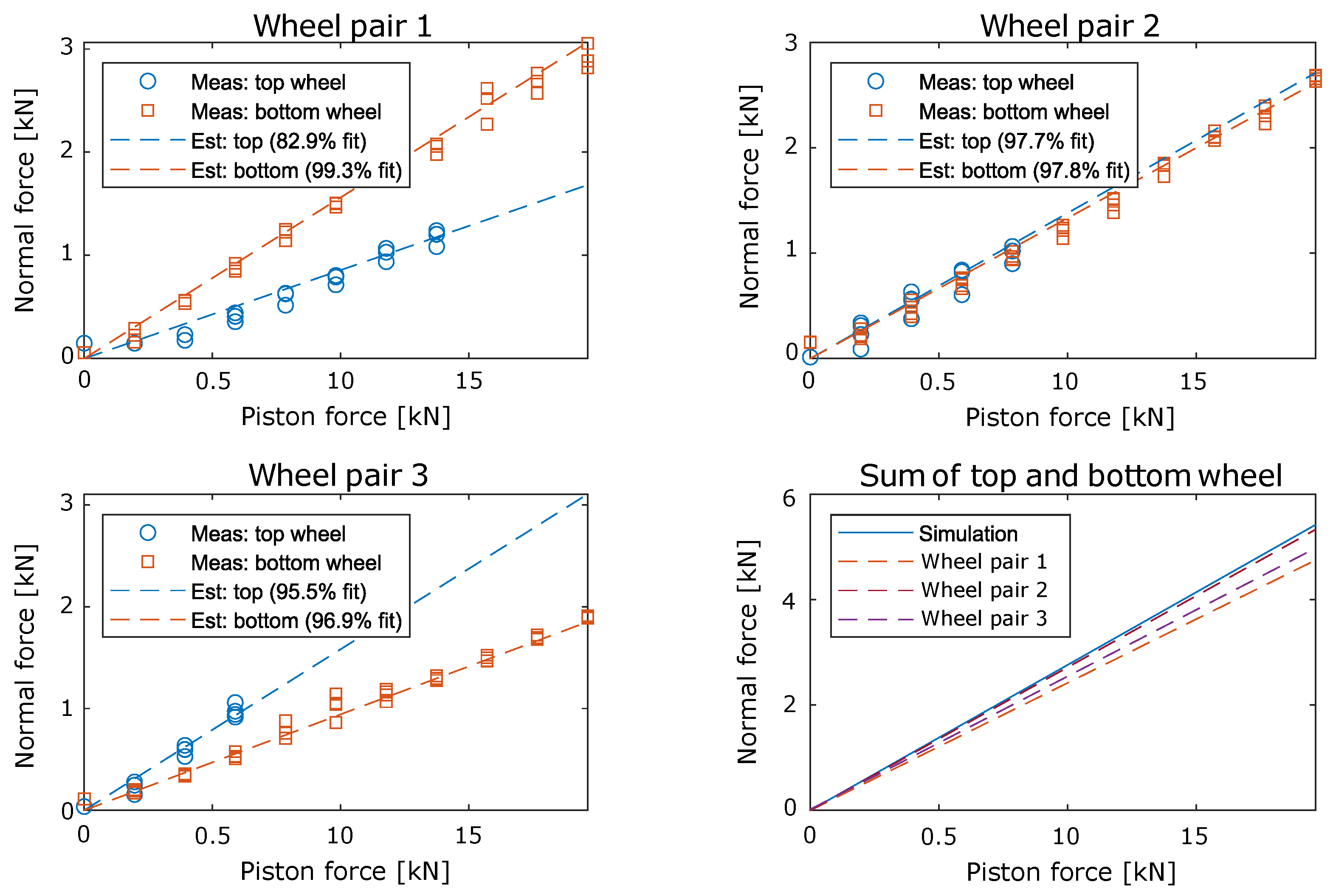
The traction force variation is due to the surface difference between the true value $F_{t,i}$ and the nominal value $F_{n,i}$ found from the real system traction curves in Figure 9. The true value is then defined with the nominal value and a state-bounded coefficient ${\varphi }_{r,i}$. The coefficient changes then depending on the road surface conditions and the relationship is described in Equation (17).

$$F_{t,i}=F_{n,i}+{\varphi }_{r,i}$$

(17)

The slip controller is designed by the differentiation of Equation (12) and substituting it with Equations (7) and (11), considering acceleration ($R_w{\omega }_i>v$) and braking ($R_w{\omega }_i<v$) in Equations (18) and (19), respectively.

$${\dot{\lambda }}_i={\dot{e}}_{\lambda ,i}={\displaystyle \frac{R_w}{J_{w}r{\omega }_i^2}}({\tau }_{c,i}-R_w{F}_{n,i}+{\overline{\tau }}_{d,i})-{\displaystyle \frac{F_{n,i}}{m_0{R}_w{\omega }_i}}-{\displaystyle \frac{\Delta v_i}{R_w{\omega }_i}}$$

(18)

$${\dot{\lambda }}_i={\dot{e}}_{\lambda ,i}={\displaystyle \frac{R_w}{J_{w}v}}({\tau }_{c,i}-R_w{F}_{n,i}+{\overline{\tau }}_{d,i})-{\displaystyle \frac{R_w{\omega }_i{F}_{n,i}}{m_0{v}^2}}-{\displaystyle \frac{R_w{\omega }_i\Delta v_i}{v^2}}$$

(19)

where $\Delta v_i$ is defined as Equation (20).

$$\Delta v_i=({\displaystyle \frac{1}{m_0}}-{\displaystyle \frac{\Delta m}{m_0(m_0+\Delta m)}})({\varphi }_{r,i}-{\displaystyle \frac{1}{3}}{F}_{roll}-{\displaystyle \frac{1}{3}}{F}_g)-{\displaystyle \frac{\Delta m}{m_0(m_0+\Delta m)}}{F}_{n,i}$$

(20)

which can be reduced to Equation (21).

$$\Delta v_i={\displaystyle \frac{{\varphi }_{r,i}-\frac{1}{3}{F}_{roll}-\frac{1}{3}{F}_g}{m}}-{\displaystyle \frac{\Delta m}{m_0(m_0+\Delta m)}}{F}_{n,i}$$

(21)

The disturbance observer, illustrated in Figure 13, estimates the ${\overline{\tau }}_{d,i}$, with the following Equation (22). The other system states of the crawler (${\theta }_c,{\dot{\theta }}_c$) as well as the velocity of each of the three wheels (${\omega }_1,{\omega }_2,{\omega }_3$) can all be measured. Therefore, they are not observed.

$${\overline{\tau }}_{d,i}={\tau }_d-r{\varphi }_{r,i}$$

(22)

using a lowpass filter to remove high-frequency components from the signal, resulting in the estimated torque ${\widehat{\overline{\tau }}}_{d,i}$.

Using the estimated ${\widehat{\overline{\tau }}}_{d,i}$, the actual traction force can be estimated as Equation (23).

$${\widehat{F}}_{t,i}={\displaystyle \frac{{\tau }_d-{\widehat{\overline{\tau }}}_{d,i}+F_{n,i}{R}_w}{R_w}}$$

(23)

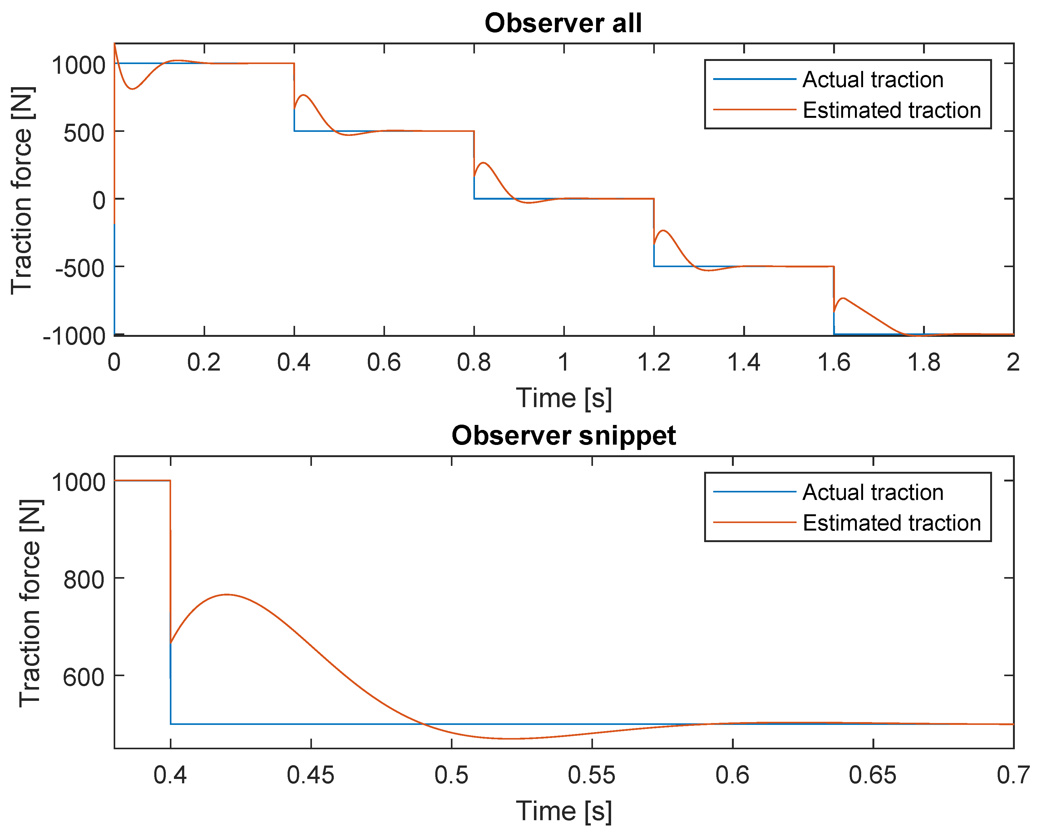
To verify the observer, it is tested in an open loop, where the input traction force is set to step down with 500 N at 0.4 s intervals visualized in Figure 14 from an original 1000 N. The observer for 1 wheel is only shown since the other 2 have the same response in the open loop.

From Figure 14, it is seen that the disturbance observer converges to the actual value after 0.15 s, with minimal overshoot. The time it takes to converge is deemed acceptable, as the crawler operational speed is at 0.05 rad/s, resulting in minimal surface change, allowing the observer to adapt during the operations. The transition period of the observer can affect the performance of the controller due to the uncertainty of the estimated traction force. When the observer is settled, the current value is maintained until the next step is applied. The observer can handle both positive and negative traction forces. Each wheel only detects the traction forces related to it, as long as there is enough traction in the system to keep the velocity constant. If all wheels simultaneously enter an area with combined insufficient traction for the crawler, the subsequent slippage from the crawler results in the individual observers being impacted by each other as they depend on the velocity of the crawler.

A control law can then be established that is able to reject disturbances as described in Equations (24) and (25).

$${\tau }_{c,i}={\overline{\tau }}_{c,i}-{\widehat{\overline{\tau }}}_{d,i}$$

(24)

$${\tau }_{c,i}=\kappa {\displaystyle \frac{k{J}_w}{R_w}}{e}_{\lambda ,i}+{\displaystyle \frac{R_w{m}_{0}v+J_w{\omega }_i}{m_{0}v}}{F}_{n,i}-{\displaystyle \frac{J_w{\omega }_i{F}_g}{3m_{0}v}}-{\rho }_r{\displaystyle \frac{e_{\lambda ,i}}{|e_{\lambda ,i}|}}-{\overline{\tau }}_{d,i}$$

(25)

where, in this case, ${\rho }_r>$0 is a design parameter, and $\kappa$ is defined as

$$\kappa ={\displaystyle \frac{{(R_w{\omega }_i+Av)}^2}{v^2{(1+A)}^2-aA{(R_w{\omega }_i-v)}^2}}$$

(26)

with

$$A=\exp (-a({\displaystyle \frac{r{\omega }_i}{v}}-1))$$

(27)

$e_{\lambda ,i}$ is determined as the difference between the current slip and the demanded slip, where ${\lambda }_d$ is the desired slip ratio, as denoted in Equation (28).

$${\lambda }_{d,i}=\left\{\begin{array}{c}{c}_d,\mathrm{if}{\lambda }_i\ge 0\\ -c_d,\mathrm{if}{\lambda }_i<0\end{array}\right.$$

(28)

Here, $c_d$ is a positive constant denoting the desired slip ratio, which is between zero and the maxima ${\mu }_{p,i}$ on the slip curves seen in Figure 9. Based on the estimated slip curves, $c_d$ is chosen with a static value of 0.07.

By substituting Equation (18) into Equation (25) and solving it with respect to $e_{\lambda ,i}$ results in Equation (29), for acceleration $R_w{\omega }_i>v$. The same can be performed for the deceleration case $R_w{\omega }_i<v$ using Equations (19) and (25) resulting in Equation (30).

$$e_{\lambda ,i}=-\kappa {\displaystyle \frac{k{v}^2}{{(R_w{\omega }_i)}^2}}{e}_{\lambda ,i}-{\displaystyle \frac{v}{J_w{R}_w{\omega }_i^2}}(\rho {\displaystyle \frac{e_{\lambda ,i}}{|e_{\lambda ,i}|}}+{\displaystyle \frac{J_w{\omega }_i\Delta v}{v}}-{\tilde{\overline{\tau }}}_{d,i})$$

(29)

$$e_{\lambda ,i}=-\kappa k{e}_{\lambda ,i}-{\displaystyle \frac{r}{J_{w}v}}(\rho {\displaystyle \frac{e_{\lambda ,i}}{|e_{\lambda ,i}|}}+{\displaystyle \frac{J_w{\omega }_i\Delta v}{v}}-{\tilde{\overline{\tau }}}_{d,i})$$

(30)

Here, the estimated error is defined as Equation (31).

$${\tilde{\overline{\tau }}}_{d,i}={\overline{\tau }}_{d,i}-{\widehat{\overline{\tau }}}_{d,i}$$

(31)

To check if the robust controller is stable, the Lyapunov stability theorem is used with the following candidate function Equation (32).

$$\mathcal{V}(e_{\lambda },i)={\displaystyle \frac{1}{2}}{e}_{\lambda ,i}^2$$

(32)

Taking the time derivative of the Lyapunov function again and using the trajectories of the closed-loop system of the robust system gives the following for acceleration in Equation (33) and braking in Equation (34).

$$\dot{\mathcal{V}}\left(e_{\lambda ,i}\right)={\dot{e}}_{\lambda ,i}{e}_{\lambda ,i}=-\kappa {\displaystyle \frac{k{v}^2}{{\left(R_w\omega \right)}^2}}{e}_{\lambda ,i}^2-{\displaystyle \frac{v}{J_w{R}_w{\omega }_i}}{e}_{\lambda }({\rho }_r{\displaystyle \frac{e_{\lambda ,i}}{|e_{\lambda ,i}|}}+{\displaystyle \frac{J_w{\omega }_i\Delta v}{v}}-{\tilde{\overline{\tau }}}_{d,i})$$

(33)

$$\dot{\mathcal{V}}\left(e_{\lambda ,i}\right)={\dot{e}}_{\lambda ,i}{e}_{\lambda ,i}=-\kappa k{e}_{\lambda ,i}^2-{\displaystyle \frac{R_w}{J_{w}v}}{e}_{{\lambda }_i}({\rho }_r{\displaystyle \frac{e_{\lambda ,i}}{|e_{\lambda ,i}|}}+{\displaystyle \frac{J_w{\omega }_i\Delta v}{v}}-{\tilde{\overline{\tau }}}_{d,i})$$

(34)

If ${\rho }_r$ in Equations (33) and (34) satisfies the following condition,

$$\overline{{\rho }_r}={\rho }_r-({\displaystyle \frac{J_w{\omega }_i\Delta v}{v}}-{\tilde{\overline{\tau }}}_{d,i})\ge 0$$

(35)

then Equations (33) and (34) can be rewritten as Equation (36), for acceleration ($R_w{\omega }_i>v$), and Equation (37) for braking ($R_w{\omega }_i<v$).

$$\dot{\mathcal{V}}\left(e_{\lambda ,i}\right)=-{\displaystyle \frac{k{v}^2{(R_w{\omega }_i+Av)}^2}{{\left(R_w\omega \right)}^2(v^2{(1+A)}^2-aA{(R_w{\omega }_i-v)}^2)}}{e}_{\lambda ,i}^2-{\displaystyle \frac{\overline{{\rho }_r}v}{J_w{R}_w{\omega }_i^2}}\left|e_{\lambda ,i}\right|$$

(36)

$$\dot{\mathcal{V}}\left(e_{\lambda ,i}\right)=-{\displaystyle \frac{k{(R_w{\omega }_i+Av)}^2}{v^2{(1+A)}^2-aA{(R_w{\omega }_i-v)}^2)}}{e}_{\lambda ,i}^2-{\displaystyle \frac{{\overline{\rho }}_r{R}_w}{J_{w}v}}\left|e_{\lambda ,i}\right|$$

(37)

So, $\dot{\mathcal{V}}(e_{\lambda },i)<0$ for both acceleration and deceleration for all $e_{\lambda ,i}\ne 0$ are stable for as long as the crawler and the wheel speeds are positive.

$${\displaystyle \frac{v}{J_w{R}_w{\omega }_i^2}}>0,{\displaystyle \frac{R_w}{J_{w}v}}>0$$

(38)

The Lyapunov function is positive-definite and decreasing, which results in $e_{\lambda ,i}$ asymptotically converging to zero. This means that the slip ratio ${\lambda }_i$ will converge to the desired slip ratio ${\lambda }_d$. The crawler can only operate in one direction since the speed always has to be positively defined. This means that the crawler can not rotate both ways without implementing a switching statement that changes what the controller perceives as the system’s positive driving direction. The change depends on the crawler’s velocity, on what it perceives as forward, as in Equation (39).

$$d=\left\{\begin{array}{c}1,\mathrm{if}v\ge 0,\left(forward\right)\\ -1,\mathrm{if}v<0,\left(backward\right)\end{array}\right.$$

(39)

In this case, the following applies, v = vd, and ${\omega }_i$ = ${\omega }_{i}d$. This ensures that it is always viewed in the positive driving direction. The change to the controller is seen in Equation (40) to ensure bidirectionality.

$${\tau }_{c,i}=d·\left(\kappa {\displaystyle \frac{k{J}_w}{R_w}}{e}_{\lambda ,i}+{\displaystyle \frac{R_w{m}_0{v}_{\mathrm{eff}}+J_w{\omega }_i}{m_0{v}_{\mathrm{eff}}}}{F}_{n,i}-{\displaystyle \frac{J_w{\omega }_i{F}_g}{3m_0{v}_{\mathrm{eff}}}}-{\rho }_r{\displaystyle \frac{e_{\lambda ,i}}{|e_{\lambda ,i}|}}-{\overline{\tau }}_{d,i}\right)$$

(40)

All the used parameters are found in

Table 5. Controller design parameters.

Parameter	k	a	${\rho }_r$	$c_d$	T
Value	6	40	20	0.07	0.03

.

7. Simulation Results

The proposed controller scheme is evaluated in simulations. Four different cases are established for PID and slip controllers with, respectively, two- and three-wheel drive. The parameter $\xi$ is used to scale the surface condition to vary the amount of traction available for the wheels. The value is changed according to

Table 6. Change in surface condition during crawler simulation at specific time intervals.

Time [s]	0	0.2	0.4	0.6	0.8
Surface condition $\mathit{\xi }$	1.33	1	0.9	0.53	1

, where the value chosen is the maximum limit where a certain controller and wheel combination can drive without slipping. A value of 1 for $\xi$ is the same as the rough surface condition from the slip curves in Figure 9.

In 2 WD, the two motors cannot deliver enough torque to overcome gravity in certain areas of the rotation. Thus, the amount of torque available for the motors in 2 WD is increased to match the total torque output from the 3 WD setup. Each motor is limited to 84 and 54 Nm in 2 WD and 3 WD, respectively. The 84 Nm is the maximum the motors can produce; hence, 1 WD is not examined as there is not enough torque available. The results of the simulation are visualized in Figure 15.

From the figure, it can be deduced that using 3 WD and the slip controller provides the largest range of surface conditions for the robot to operate on. The supervisor is enabled when the slip threshold is crossed at 0.6 s for 3 WD. The supervisor reduces the slip to the demanded slip ratio in order to optimize traction. At this point, the supervisor is disabled at the 0.8 s mark, where surface conditions change to the nominal surface. The PID-only controller case has a slip ratio of $\lambda =1$ and only recovers when the surface traction is increased again.

The spike seen in the torque on the individual wheels before 0.6 s is due to sensor noise added to the system. This noise causes the slip controller to experience the crawler slipping while it is actually not. This is normally not an issue for cars, as they move at much higher velocities, so the effect on slip calculations is negligible. As the slip controller chatters, the plotted torque is also filtered with a moving average using a window of 50 samples.

8. Physical Tests

To finalize this study, the proposed mechanical and control changes will be implemented on the physical robot and tested in a physical test environment as presented in Section 4.

While the test surfaces used in this study were designed to replicate a range of traction conditions representative of offshore environments, it is important to note that all physical tests were conducted in a dry and controlled laboratory setting. Environmental factors such as salt water, corrosion, and biofouling were not included. These conditions can significantly affect sensor reliability and surface interaction.

The performance of the robot is evaluated based on the distance traveled, the combined absolute mean slip ($|\overline{\lambda }|$), the Integrated Absolute Error (IAE) of the velocity, and the Mean Absolute Control Input (MEACI). The average slip is presented as a total average between all three wheels, and the MEACI is calculated from the sum of the actuated wheels normalized as depicted in Equation (41).

$$\mathrm{MEACI}={\displaystyle \frac{1}{n}}\sum _{i=1}^n\left|{\tau }_{c,nom,i}\right|$$

(41)

where n is the number of samples. The IAE as described in Equation (42) is compared to the reference of 0.05 rad/s and is normalized according to the time duration of each test.

$$\mathrm{IAE}=\sum _0^n\left|e_{\omega }\left(n\right)\right|$$

(42)

8.1. Surface Tests

Three cases are designed to test for varying surfaces:

• Nominal case (NOM): Performed on a rough painted surface seen in Figure 4, this surface is intended to rotate the crawler with a minimum amount of slip, used for comparison.
• Surface case 1 (S1): Performed on a smooth painted surface seen in Figure 4, this surface is assumed to work with some slip in certain scenarios.
• Surface case 2 (S2): Performed on a smooth painted surface with the clamping force reduced by 40% in order to reduce traction. This surface is assumed to show a worst-case scenario.

The tests are performed in an order in which all operational and mechanical setups are tested, starting with the nominal surface and proceeding to the test surfaces.

Based on the simulation results presented in Section 7, it is found that the 1 WD setup of the crawler is not able to overcome gravity on the setup. Hence, this setup is not tested, and no results are presented in the following sections. For the constant torque test (CT), the chosen values were 84 and 54 for 2 WD and 3 WD. These values were chosen to ensure that the total torque input in these operations is comparable.

8.2. Results

The results shown in this section evaluate the performance of the robot based on either the mechanical configuration (2 WD and 3 WD) as well as the combination of using a manual control input versus either a nominal controller or an advanced slip detection controller. The results are presented as time plots showing results from the three surface types (NOM, S1, and S2), and the statistical features of all performed tests are then compared. To remove the effect of noise on the figures, a moving average filter with a 50-sample averaging window is used.

8.2.1. NOM Surface Tests

Six tests are performed on the NOM surface, and the results are compared in Figure 16, showing the different controllers and wheel configurations.

Comparing the velocity output from the robot in the tests on the NOM surface, it can be seen that both the PID and the slip controller are able to track the velocity reference of 0.05 rad/s. It is visible that when going from 3 WD to 2 WD, the window of tracking the velocity is reduced. The 2 WD and 3 WD tests with no control effort do not track the velocity reference. The CT on 2 WD is not able to overcome gravity, and it can be seen that the velocity in this test comes to a halt at 8.5 s. The same is depicted for the 2 WD PID and SLIP at 12.5 and 18 s, respectively. When comparing the slip on the individual wheels, it is visible that for 2 WD the amount of slip is increased on wheels 1 and 3 compared to 3 WD. In the 3 WD test with manual input, it is seen that at 18 s, wheel 2 is stuck, thus preventing the crawler from moving forward from this point.

8.2.2. S1 and S2 Surface Tests

The second set of tests is performed on the changed surface conditions, S1 and S2. The crawler was not able to initiate a rotation without slipping in 2 WD operation on surface S2; hence, these tests are not included.

From Figure 17, when comparing velocities, it can be deduced that the tests, including controllers, are able to track the velocity within the set boundaries. For the 2 WD tests, it can be seen that the amount of time in which the controllers can track the velocity is reduced. Comparing the individual slips, it is discovered that the slip is increased when operating in 2 WD. In 3 WD, the slip is most noticeable at wheel 2l this was also visually confirmed during the tests.

From Figure 18, it is seen that when comparing velocities, the PID is able to maintain a constant velocity within the boundaries, whereas the SLIP is able to maintain a velocity within the boundaries until 7 s. At this point, the controller loses all traction, and the velocity is reversed due to the gravitational pull. At 13 s, it can be seen that the SLIP test is not able to regain traction, and as visualized on the slip curves of wheel 2, a constant slip is measured. The CT test is able to reach within the velocity boundaries; however, as the crawler is rotated, the gravitational pull becomes too high, and a slip close to 1 is found at both wheels one and two. A summary of the important statistical features of the tests is compared in

Table 7. Comparison of performance of the two robot setups in open loop, nominal control, and slip control on the nominal surface and the two test surfaces.

		2 WD				3 WD
Controller	Surface	$|\overline{\mathbf{\lambda }}|$	Distance [rad]	IAE	MEACI	$|\overline{\mathbf{\lambda }}|$	Distance [rad]	IAE	MEACI
	NOM	0.73	0.25	1.38	1.08	0.64	0.80	2.06	2.56
None	S1	0.89	0.29	1.30	0.92	0.30	1.43	2.32	4.12
	S2	-	-	-	-	0.70	0.27	3.32	2.25
	NOM	0.66	0.40	1.36	1.65	0.18	1.27	0.30	3.38
PID	S1	0.78	0.49	2.46	3.32	0.24	1.55	0.24	3.96
	S2	-	-	-	-	0.70	1.10	0.37	2.31
	NOM	0.69	0.38	2.32	2.32	0.60	1.30	0.41	3.19
SLIP	S1	0.83	0.40	3.38	4.40	0.63	1.47	0.44	3.44
	S2	-	-	-	-	0.59	0.20	1.20	0.53

.

Comparing the results from Table 7, it can be seen that across all setups, the 3 WD configuration outperforms the 2 WD setup in terms of the distance traveled, IAE, and MEACI. However, when looking into the average amount of energy per rad distance in 2 WD compared to 3 WD ignoring S2, there is a reduction of 7.04% with using 2 WD instead of 3 WD. This can be beneficial for long-term operations but is not the main outcome of this paper. It provides the foundations for a techno-ecological analysis, both by having fewer motors and less power consumption, but it needs to be put in relation to the rest of the operational costs and performance aspects. The slip controller generally results in the highest IAE and MEACI values, suggesting that it requires more control effort to maintain stable slip. For the S2 surface, the 2 WD setup fails to operate effectively, while the 3 WD configuration is still able to maintain traction and control, though with increased effort.

8.2.3. 2 WD

In the 2 WD setup, both the PID and slip controllers show significant slip across all surfaces, with S1 and NOM having values between 0.66 and 0.83. This indicates higher slip, which limits the robot’s ability to track the velocity reference accurately, as shown by the higher IAE values. For the NOM surface, the 2 WD setup travels the least distance (0.25 to 0.49 rad) and demonstrates limited ability to overcome environmental challenges, like gravity or reduced traction. The 2 WD setup consistently has lower MEACI values, which reflects less control effort, but this also comes with a trade-off in performance, especially under difficult conditions.

8.2.4. 3 WD

The 3 WD setup consistently performs better than the 2 WD setup, achieving lower slip values, greater distance traveled, and improved tracking accuracy. For instance, on the NOM surface with PID control, it achieves $|\overline{\lambda }|$ of 0.18 and travels 1.27 rad compared to 0.66 and 0.40 rad in 2 WD. On the S1 surface, the 3 WD setup with the slip controller achieves a lower slip and better velocity tracking compared to the 2 WD setup. Even on the challenging S2 surface, the 3 WD setup performs adequately, although slip increases slightly with the slip controller, which still allows the crawler to cover some distance.

8.2.5. Controllers

The slip controller, while effective in managing slip, incurs the highest control effort and results in higher IAE values in most cases, indicating that it needs more intensive adjustments to maintain control in more complex conditions, like S1 and S2. The PID controller strikes a balance between accuracy and control effort. This results in lower slip and better tracking on the NOM surface but under-performs slightly on more challenging surfaces like S1 and S2 compared to the slip controller. The open-loop setup has the poorest performance, especially on the S1 and S2 surfaces, where it struggles to maintain traction, resulting in higher slip and poor velocity tracking.

9. Conclusions

This work examined the different aspects of preventing slip from occurring on an offshore external pipe crawling robot. This involved upgrading the existing robot with MWD and increasing its autonomy with sensors and a control unit with an ROS. Two models describing the dynamics of the robot was developed. The traction force between the surface and the robot was described using the magic formula and the unknown parameters were determined using the Linear Least Squares method from the experimental data. A nominal and experimental controller was developed and tested in simulation before being implemented and validated using physical experiments. The supervising slip controller had a disturbance observer to detect changes in driving conditions caused by biofouling on the member. The requirement for all three wheels to have this feature is attributable to the crawler’s slow operational speeds, where all wheels cannot be assumed to drive on the same surface.

From the simulations, it is visible that the extra slip control increases the crawler’s ability to operate on worse surfaces, as well as running 3 WD compared to 2 WD. When practically implemented, the slip controller managed the slip but caused chattering, which resulted in a higher control effort seen in the IAE. The best way to improve is with using 3 WD compared to 2 WD, increasing redundancy should one wheel lose traction. This sometimes caused it to be unable to start up with only 2 WD and, therefore, constantly slipping. However, 2 WD was 7.04% more energy efficient. Thus, the most effective way to prevent slipping is to increase the piston pressure, thereby improving available traction through mechanical means (MWD). If further performance improvements are needed, the implementation of slip control can offer benefits in certain conditions. However, as demonstrated by its failure to drive on S2 and its higher control torque and computational requirements, it does not provide advantages in all scenarios. Overall, the integration of 3 WD and slip control offers a robust solution for offshore inspection and maintenance operations, where environmental factors such as surface irregularities and biofouling pose challenges. The results highlight the importance of advanced control systems in enhancing the operational efficiency and safety of crawler robots. Future research should focus on further optimizing these control mechanisms and exploring the scalability of these solutions for other types of offshore infrastructure, ensuring continued advancements in offshore robotics technology. To further utilize the GPU capabilities of the Jetson, real-time image processing and AI-based methods for adaptive slip estimation could be investigated. Techniques such as fuzzy logic or maximum power point tracking (MPPT) could be implemented to dynamically determine the optimal slip ratio based on surface conditions.

For future reference, an investigation of alternative wheel configurations, such as ball wheels or omnidirectional systems, to enable more flexible traversal in complex offshore geometries should be performed.

References

1. Fazeres-Ferradosa, T.; Rosa-Santos, P.; Taveira-Pinto, F.; Vanem, E.; Carvalho, H.; Correia, J. Advanced research on offshore structures and foundation design: Part 1. Marit. Eng. 2019, 172, 118–123. [Google Scholar] [CrossRef]
2. Sharp, J.V. Underwater Inspection and Repair for Offshore Structures; John Wiley & Sons, Inc.: Hoboken, NJ, USA, 2021. [Google Scholar]
3. Othman, N.A.; Mohd, M.H.; A Rahman, M.A.; Musa, M.A.; Fitriadhy, A. Investigation of the corrosion factor to the global strength of aging offshore jacket platforms under different marine zones. Int. J. Nav. Archit. Ocean. Eng. 2023, 15, 100496. [Google Scholar] [CrossRef]
4. Shukla, A.; Karki, H. Application of robotics in offshore oil and gas industry—A review Part II. Robot. Auton. Syst. 2016, 75, 508–524. [Google Scholar] [CrossRef]
5. Fahrni, L.; Thies, P.R.; Johanning, L.; Cowles, J. Scope and feasibility of autonomous robotic subsea intervention systems for offshore inspection, maintenance and repair. In Advances in Renewable Energies Offshore, Proceedings of the 3rd International Conference on Renewable Energies Offshore, RENEW 2018, Lisbon, Portugal, 8–10 October 2018; CRC Press: London, UK, 2019; pp. 771–778. [Google Scholar] [CrossRef]
6. Sub-C Partner. The “Spider Deck Clean-Up” Campaign. Available online: https://www.subcpartner.com/news/the-spider-deck-clean-up-campaign-tyra (accessed on 30 September 2023).
7. Nordin, M.H.; Sharma, S.; Khan, A.; Gianni, M.; Rajendran, S.; Sutton, R. Collaborative Unmanned Vehicles for Inspection, Maintenance, and Repairs of Offshore Wind Turbines. Drones 2022, 6, 137. [Google Scholar] [CrossRef]
8. Shafiee, M.; Zhou, Z.; Mei, L.; Dinmohammadi, F.; Karama, J.; Flynn, D. Unmanned aerial drones for inspection of offshore wind turbines: A mission-critical failure analysis. Robotics 2021, 10, 26. [Google Scholar] [CrossRef]
9. Tena, I. Automating ROV Operations in Aid of the Oil & Gas Offshore Industry. Technical Report. August 2011. Available online: https://www.unmannedsystemstechnology.com/wp-content/uploads/2013/10/White-Paper-Automating-ROV-Operations.pdf (accessed on 2 September 2023).
10. Isnadi, B.; Lee, L.A.; Ng, S.M.; Suhaili, A.S.; Nasir, Q.R.M.; Sham, H.; Puloh, K.P.; Omar, S.; Saminal, S.N.; Lihin, Z.H.; et al. A Hybrid Topside Structural Approach to the Management of Aging Fleet. In Proceedings of the International Petroleum Technology Conference, IPTC 2021, Virtual, 23 March–1 April 2021. [Google Scholar] [CrossRef]
11. Hooft Graafland, C.; Jovanova, J. From Heights to the Deep Sea, a Review of Robots Interacting with Offshore Structures. Robot. Rep. 2024, 2, 85–100. [Google Scholar] [CrossRef]
12. Sarkar, A.; Gudmestad, O.T. Splash zone lifting analysis of subsea structures. In Proceedings of the International Conference on Offshore Mechanics and Arctic Engineering—OMAE, Shanghai, China, 6–11 June 2010; Volume 1, pp. 303–312. [Google Scholar] [CrossRef]
13. V Tecchio, P.P.; Vieira, M.; Batista, L.; Cerqueira, J.; Lima, R.; Pinheiro, O.; Nardy, L.; dos Reis, M.A.; Lepikson, H.; M Lopes, L.F. Overview of Robotic Applications on Offshore OGI IMR: Splash Zone. In Proceedings of the OCEANS 2021: San Diego–Porto, San Diego, CA, USA, 20–23 September 2021. [Google Scholar]
14. Ho, M.; El-Borgi, S.; Patil, D.; Song, G. Inspection and monitoring systems subsea pipelines: A review paper. Struct. Health Monit. 2020, 19, 606–645. [Google Scholar] [CrossRef]
15. Xue, J.; Chen, J.; Stancu, A.; Wang, X.; Li, J. Spatial Trajectory Tracking of Wall-Climbing Robot on Cylindrical Tank Surface Using Backstepping Sliding-Mode Control. Micromachines 2023, 14, 548. [Google Scholar] [CrossRef] [PubMed]
16. Medeiros, V.S.; Kubrusly, A.C.; Bertoche, R.L.; Freitas, M.A.; Camerini, C.; Brito, J.L.F.; von der Weid, J.P. Automatic tool with adaptive suspension system for high-quality inspection of underwater risers. Ind. Robot. 2021, 48, 442–453. [Google Scholar] [CrossRef]
17. OceanTech. Customised Solutions for All Cleaning and Inspection Needs in the Splash Zone. Available online: https://oceantech.no/splash-zone-network/articles/customised-solutions-for-all-cleaning-and-inspection-needs-in-the-splash-zone/ (accessed on 10 October 2023).
18. Frantz, J.C. Advances in Robotic Technology for Splash Zone Inspection: A Comprehensive Research. November 2024. Available online: https://www.researchgate.net/publication/385508756_ADVANCES_IN_ROBOTIC_TECHNOLOGY_FOR_SPLASH_ZONE_INSPECTION_A_COMPREHENSIVE_RESEARCH (accessed on 3 March 2025).
19. Chatzakos, P.; Papadmitriou, V.; Psarros, D.; Nicholson, I.; Gan, T.H. On the development of an unmanned underwater robotic crawler for operation on subsea flexible risers. In Proceedings of the 2010 IEEE Conference on Robotics, Automation and Mechatronics, RAM 2010, Singapore, 28–30 June 2010; pp. 419–424. [Google Scholar] [CrossRef]
20. Gotts, C.; Hall, B.; Beaumont, O.; Chen, Z.; Cleaver, W.; England, J.; White, D.; Thornton, B. Development of a prototype autonomous inspection robot for offshore riser cables. Ocean. Eng. 2022, 257, 111485. [Google Scholar] [CrossRef]
21. Schultz, M.P. Frictional resistance of antifouling coating systems. J. Fluids Eng. Trans. ASME 2004, 126, 1039–1047. [Google Scholar] [CrossRef]
22. Candries, M. Drag, Boundary-Layer and Roughness Characteristics of Marine Surfaces Coated with Antifoulings. Ph.D. Thesis, University of Newcastle-upon Tyne, Newcastle, UK, 2001. [Google Scholar]
23. Sub-C Partner. The Robotic Crawler. Available online: https://www.subcpartner.com/assets/Dokumenter/1247811c8b/Crawler-brochure.pdf (accessed on 1 September 2023).
24. Fang, G.; Cheng, J. Design and Implementation of a Wire Rope Climbing Robot for Sluices. Machines 2022, 10, 1000. [Google Scholar] [CrossRef]
25. Pretagostini, F.; Ferranti, L.; Berardo, G.; Ivanov, V.; Shyrokau, B. Survey on Wheel Slip Control Design Strategies, Evaluation and Application to Antilock Braking Systems. IEEE Access 2020, 8, 10951–10970. [Google Scholar] [CrossRef]
26. Liebemann, E.K.; Meder, K.; Schuh, J.; Nenninger, G. Safety and Performance Enhancement: The Bosch Electronic Stability Control (ESP). Technical Report. 2004. Available online: https://www.sae.org/publications/technical-papers/content/2004-21-0060/ (accessed on 10 October 2023).
27. Becker Jensen, H.C. Design of Slip-Based Active Braking and Traction Control System for the Electric Vehicle QBEAK. Ph.D. Thesis, Aalborg University, Esbjerg, Denmark, 2012. [Google Scholar]
28. Subroto, R.K.; Wang, C.Z.; Lian, K.L. Four-Wheel Independent Drive Electric Vehicle Stability Control Using Novel Adaptive Sliding Mode Control. IEEE Trans. Ind. Appl. 2020, 56, 5995–6006. [Google Scholar] [CrossRef]
29. Korayem, M.; Safarbali, M.; Lademakhi, N.Y. Adaptive robust control with slipping parameters estimation based on intelligent learning for wheeled mobile robot. ISA Trans. 2024, 147, 577–589. [Google Scholar] [CrossRef] [PubMed]
30. Zhang, L.; Wang, B.; Guan, E.; Liu, X.; Saqib, M.; Zhao, Y. Adaptive Skid-Steering Control Approach for Robots on Uncertain Inclined Planes with Redundant Load-Bearing Mobility. Biomimetics 2024, 9, 64. [Google Scholar] [CrossRef] [PubMed]
31. Nguyen, B.M.; Hosomi, Y.; Sato, T.; Morimoto, Y.; Mizuguchi, T.; Oda, M.; Toyota, H.; Nagai, S.; Fujimoto, H. Driving Force Control for Electric Vehicles: A Survey on Its Origin, Developments, and Future Trends. 2025. Available online: https://www.researchgate.net/profile/Binh-Minh-Nguyen/publication/390221978_Driving_Force_Control_for_Electric_Vehicles_A_Survey_on_Its_Origin_Developments_and_Future_Trends/links/67e4f1cef966c17052a73e52/Driving-Force-Control-for-Electric-Vehicles-A-Survey-on-Its-Origin-Developments-and-Future-Trends.pdf (accessed on 2 March 2025).
32. Ikeda, Y.; Nakajima, T.; Chida, Y. Vehicular slip ratio control using nonlinear control theory. IFAC Proc. Vol. 2011, 44, 8403–8408. [Google Scholar] [CrossRef]
33. Amodeo, M.; Ferrara, A.; Terzaghi, R.; Vecchio, C. Wheel slip control via second-order sliding-mode generation. IEEE Trans. Intell. Transp. Syst. 2010, 11, 122–131. [Google Scholar] [CrossRef]
34. Genta, G. Motor Vehicle Dynamics. Modeling and Simulation; World Scientific: Singapore, 1997. [Google Scholar]
35. Besselink, I.J.; Schmeitz, A.J.; Pacejka, H.B. An improved Magic Formula/Swift tyre model that can handle inflation pressure changes. Veh. Syst. Dyn. 2010, 48, 337–352. [Google Scholar] [CrossRef]
36. Bakker, E.; Pacejka, H.B.; Lidner, L. A New Tire Model with an Application in Vehicle Dynamics Studies. J. Passeng. Cars 1989, 98, 101–113. [Google Scholar]
Figure 1. An overview of the major components used for designing one of the clamps for the crawler.
Jmse 13 00777 g001
Figure 2. Position of hardware on the crawler.
Jmse 13 00777 g002
Figure 3. Connections between the various hardware components, with EPOS4-(5-7) being the CAN Bus ID. Voltage connections are shown in red, motor feedback in purple, and CAN communication lines in yellow (high) and blue (low).
Jmse 13 00777 g003
Figure 4. Nominal (rough) and comparison (smooth) test surfaces seen left and right, respectively.
Jmse 13 00777 g004
Figure 5. The crawler attached to the horizontally oriented test member.
Jmse 13 00777 g005
Figure 6. The experimental setup for normal forces for the vertical member position.
Jmse 13 00777 g006
Figure 7. Free-body diagram of the crawler attached to a member seen from the side. The force balance of the crawler is divided into six sections: (1) input piston force, (2) wheel 2 section, (3) left moment arm, (4) right moment arm, (5) left claw and wheel 1 section, and (6) right claw and wheel 3 section.
Jmse 13 00777 g007
Figure 8. The force measurement on each of the wheel pairs. Note that no top wheel measurements go above 5 kN. This is due to the limitations of the HBM C8C load cells.
Jmse 13 00777 g008
Figure 9. Figure describing the traction relationship with slip for each wheel: (a) wheel 1 traction curve, (b) wheel 2 traction curve, and (c) wheel 3 traction curve. Green and blue dashed lines highlight the intersections of the braking and acceleration peaks, respectively.
Jmse 13 00777 g009
Figure 10. Comparison of angular velocity and position between measurements and simulations.
Jmse 13 00777 g010
Figure 11. Control design block diagram structure of slip controller for individual wheels.
Jmse 13 00777 g011
Figure 12. Comparison between approximate slip and real slip, with a = 40 .
Jmse 13 00777 g012
Figure 13. Block diagram of the disturbance observer.
Jmse 13 00777 g013
Figure 14. Traction force estimation, with the available amount of traction decreasing by 500 N every 0.4 s.
Jmse 13 00777 g014
Figure 15. Comparison between PID and slip controller with 2 WD and 3 WD in angular velocity, torque, and slip, with torque having a moving average of 50.
Jmse 13 00777 g015
Figure 16. Comparing crawler velocity and individual wheel slip of MWD and controller setup on NOM surface.
Jmse 13 00777 g016
Figure 17. Comparing crawler velocity and individual wheel slip of MWD and controller setup on S1 surface.
Jmse 13 00777 g017
Figure 18. Comparing crawler velocity against reference velocity (black dashed line), and presenting individual wheel slip when for varying MWD and controller setup on S2 surface. Note that the velocity of the 2 WD tests is zero on this surface; therefore, their respective slip ratios are not estimated and are not included in the figures.
Jmse 13 00777 g018