1. Introduction
The rapid development of the shipping industry has significantly enhanced its role in economic globalization. As of January 2023, the global fleet consisted of 105,493 vessels with a gross tonnage of 100 tons or more [
1]. However, the environmental pollution and health risks associated with ship emissions cannot be overlooked [
2]. The pollutants released by ships include sulphur oxides (SOx), nitrogen oxides (NOx), particulate matter (PM), volatile organic compounds (VOCs), black/elemental carbon (BC/EC), and organic carbon (OC) [
3]. Notably, carbon dioxide (CO
2) is the most prevalent emission; however, it is generally classified as a greenhouse gas. Relevant studies indicate that these pollutants emitted by ships have a significant impact on the environmental ecology and human health in coastal port cities [
4,
5,
6,
7].
Utilizing onboard scrubbers on vessels can effectively mitigate sulphur emissions; however, this approach may lead to an increase in the emissions of other pollutants [
8]. Operational alternatives, such as optimizing maritime routes, can effectively reduce emissions at a low cost. However, comprehensive long-term emission reduction strategies remain essential [
9]. In recent years, numerous researchers have demonstrated that limiting the FSC in marine fuel oil can not only directly reduce the amount of SOx emitted during fuel combustion but also indirectly decrease particulate matter (PM) emissions. This approach serves as an effective means to mitigate pollution generated by ships [
10,
11,
12]. Consequently, the International Maritime Organization (IMO) has proposed establishing a cap on the sulphur content of global ship fuel oil, with a global FSC limit set at 0.50% (m/m) since 2020. Furthermore, the IMO has designated four ship emission control areas—namely, the Baltic Sea, North Sea, North American region, and United States Caribbean Sea—where vessels are required to utilize fuels with lower sulphur content; within these areas, the FSC limit has been maintained at 0.10% (m/m) since 2015 [
13].
Additionally, some countries (e.g., China) have implemented domestic ship emission control areas aimed at reducing the adverse effects of ship emissions within their regions. However, effectively promoting compliance with policies governing ship emission control areas necessitates oversight from relevant maritime authorities regarding the fuels utilized by vessels operating under their jurisdiction. While accurate detection of FSC can be achieved through direct extraction of oil samples from ships, this method is characterized by low efficiency and randomness and incurs high labour costs.
Therefore, several studies have proposed estimating Fuel Supply Consumption (FSC) by monitoring ship emissions [
14,
15,
16,
17]. The measurement techniques for analyzing a ship’s smoke plume can be categorized into optical methods [
18,
19,
20,
21] and sniffer methods [
22,
23]. Among these approaches, optical methods—such as differential optical absorption spectroscopy, light detection and ranging, and ultraviolet camera—analyze the changes in light properties following their interaction with the exhaust plume. If the local wind field is known, these methods enable the determination of sulphur dioxide (SO
2) emission rates. However, simultaneous measurements of carbon dioxide (CO
2) are not feasible using this approach; thus, it becomes impossible to ascertain fuel consumption accurately and derive a more precise FSC value. In contrast, sniffer methods rely on concurrent measurements of elevated CO
2 and SO
2 concentrations within a ship’s exhaust plume. The measurement of CO
2 facilitates the assessment of SO
2 emissions based on the amount of fuel burned at any given time. This allows for direct estimation of FSC through the SO
2-CO
2 ratio [
24]. Evidence from numerous field comparisons indicates that more accurate FSC results can be achieved with sniffer methods since they directly measure the characteristics of the ship’s smoke plume [
25,
26].
In the context of maritime supervision, the sniffer method can be categorized into two types based on data collection techniques: mobile measurements and fixed measurements. The former involves unmanned aerial vehicles (UAVs), aircraft, helicopters, and ships equipped with sniffer technology that actively enter the plume to measure gas concentrations [
27,
28,
29,
30,
31]. In contrast, fixed measurements entail installing sniffer equipment on land-based structures such as shores, bridges, or wharves—referred to in this study as the land-based sniffer method—to passively monitor gas emissions from passing vessels. This approach enables continuous and real-time online monitoring [
32], making it applicable in numerous port areas [
33,
34].
Recent studies have indicated that, despite the implementation of Emission Control Area (ECA) policies, some ships continue to exceed the allowable limits for FSC. Van Roy et al. (2022) utilized small aircraft equipped with sniffer monitoring devices to effectively assess 4592 ship plumes in the Belgian North Sea from 2015 to 2019 [
35]. Throughout this operational period, the overall compliance rate was found to be 92%. Similarly, Zhou et al. (2022) employed Unmanned Aerial Vehicles (UAVs) outfitted with sniffer equipment to monitor 30 vessels in the Waigaoqiao area of China in 2021 [
32]; among these, 8 were identified as having FSC levels exceeding 0.50% (m/m). Furthermore, Qi et al. (2023) conducted land-based monitoring using sniffer technology on six ships at Tianjin Port, China, also in 2021 [
34]; one of these vessels was confirmed to have an FSC above the threshold of 0.50% (m/m). Additionally, numerous other sniffer measurements across Europe further underscore both the effectiveness and practicality of utilizing sniffing techniques for measuring ship exhaust emissions [
36,
37]. Overall, land-based sniffer methods have been implemented to a significant extent and have proven effective for monitoring FSC levels.
Existing monitoring activities have gradually been transitioned to routine operations in many locations. However, due to the complexities of the external environment, the mutual interference from multiple ship emissions, and the influence of vehicles and tugboats within port areas, the collected exhaust gas data exhibit several issues. These include large data volumes, high redundancy, abnormal readings, and challenges in distinguishing emission sources. Such problems significantly hinder FSC monitoring and ship identification efforts. Therefore, to address the difficulties associated with measuring FSC in complex port environments and to assist the Maritime Safety Administration in enhancing regulatory efficiency, this study proposes a ship emission monitoring approach specifically designed for FSC measurements under these challenging conditions.
Section 2 presents specific calculation methods and system design. The experiment, results, and applications are detailed in
Section 3, while conclusions are drawn in
Section 4.
2. Method
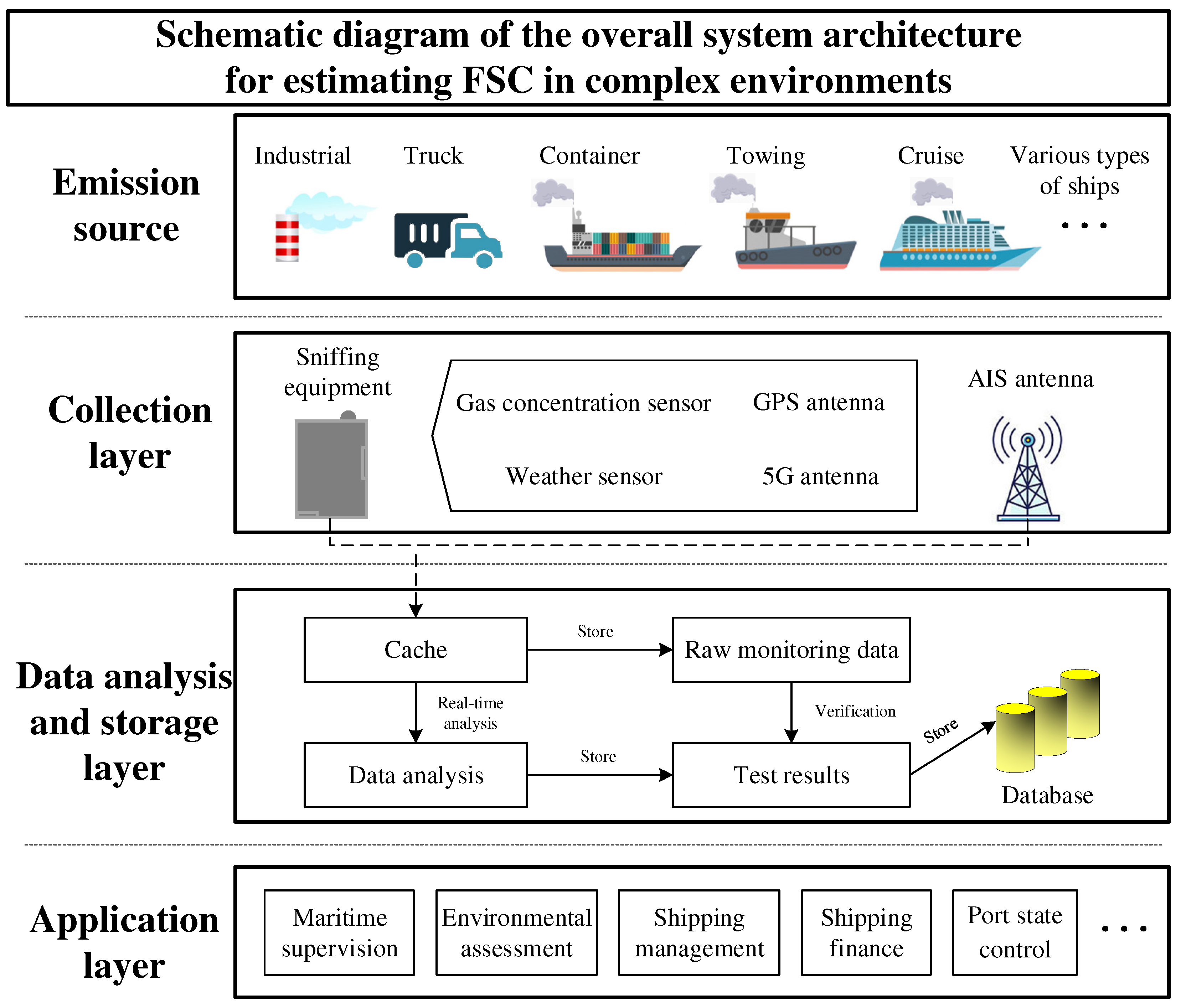
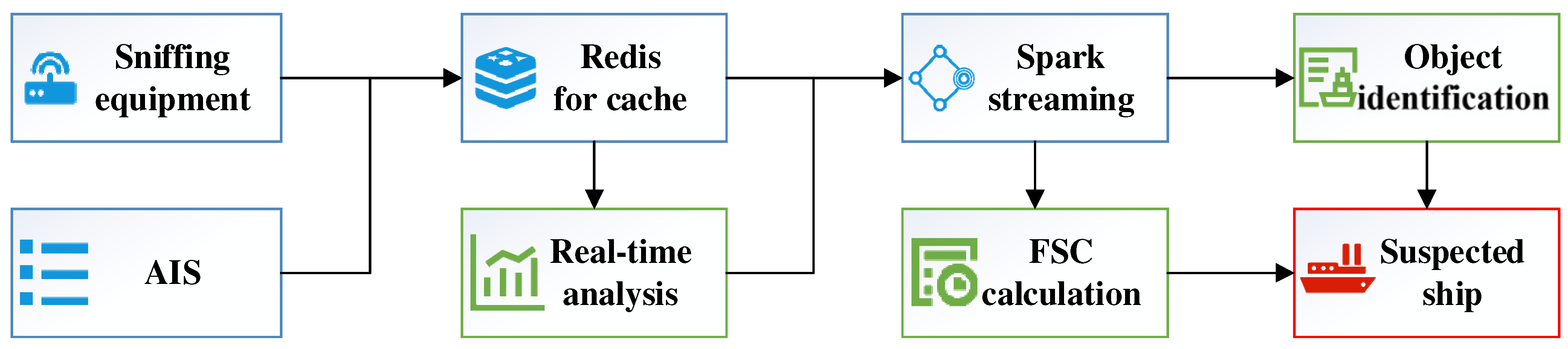
In this study, we designed the system architecture shown in
Figure 1. At the emission source level, seagoing and inland river ships berthed or maneuvered in port areas are subject to FSC monitoring. Container trucks and tugs are port enterprises that generally meet emission requirements using diesel as fuel; however, they are also very active objects in dock areas, and the exhaust gas emitted may be collected by the monitoring equipment, which interferes with FSC estimations of ships. In addition, there may be industrial emission sources around port areas that increase the background value of polluting gases in the environment.
The acquisition layer was mainly composed of an automatic identification system (AIS) base station and sniffer monitoring equipment, and an AIS antenna was responsible for collecting AIS signals broadcast in the surrounding waters to obtain information such as ship name, call sign, position, speed, and heading. The sniffer monitoring equipment mainly consisted of four modules: gas-concentration-measurement sensor module (SO2, NO2, CO2), meteorological five-element-measurement sensor module (temperature, humidity, air pressure, wind speed, and direction), GPS antenna, and 5G antenna. The real-time measured data are transmitted via the 5G network to the cloud server in the analysis and storage layers. Because the collected data were real-time data, analysis of the FSC of the ship required a period of measured values; therefore, a cache module was designed to collect the data uploaded by the acquisition layer. A real-time analysis of the data in the cache was performed to obtain the monitoring results, and the data in the cache were refreshed and written into the database at a certain time interval as the original data for subsequent verification. At the application level, the monitoring results can be associated with the route information of a ship, technical information, energy demand information, and other data sources via call signs in the AIS, which can be used in maritime supervision, environmental assessment, shipping management, shipping finance, and other applications.
In the data analysis process, FSC was calculated based on the sniffer method principle, as shown in Equation (1).
Here, FSC represents the sulphur content of the fuel; % is the percentage of mass;
S is the mass of sulphur in the fuel; and fuel is the fuel mass. The marine fuel carbon content is 87 ± 1.5% [
38]. After combustion, sulphur and fuel oil are converted into SO
2 and CO
2.
A(
S) and
A(
C) are the molar masses of sulphur and carbon, respectively, and the coefficient is 0.232 after the above parameters are substituted [
39]. R indicates the conversion of sulphur elements to sulphur oxides such as SO
3 and H
2SO
4 after combustion [
40]. SO
2 and CO
2 are diluted by wind-borne advection; however, the proportion remains unchanged within a certain range, and the difference in the sedimentation rate caused by molecular weight differences can be neglected during wind-borne diffusion. Therefore, the FSC was estimated by measuring ship plumes’ SO
2 and CO
2 concentrations. Because SO
2 and CO
2 are also present in the air, the ratio of SO
2 to CO
2 was obtained by subtracting the background value (bkg) from the peak value. In addition, owing to the difference in the sensor response time between SO
2 and CO
2, to reduce the large uncertainty caused by a single measurement value, the measured values within a period are generally integrated and summed; that is, the FSC calculation is performed using the area ratio of the peak area.
The method in Equation (1) has been widely used in UAV and aircraft platforms equipped with sniffer equipment to take the initiative to fly into the smoke plume of ship targets for measurements [
35]. There has been some research on land-based sniffer methods [
41], monitoring equipment is generally located on the shore beside a channel or on a bridge in an inland river, and generally only analyses the individual ship targets passing by the surrounding area. Although the sniffer method subtracts the background values form the peak values to identify and allocate an individual ship, it is difficult to effectively deal with the complex emission environment in the port terminal area. Therefore, this study designed a caching mechanism based on the “Redis + Spark Streaming” technology [
42] and preliminarily determined whether subsequent FSC calculations could be carried out based on measured gas concentration and AIS data to meet the computational requirements of real-time data reception and analysis. The data in the cache were then used to dynamically calculate the SO
2 to CO
2 background values to eliminate the influence of other emission sources on the monitoring effect. Subsequently, the ship plume event in the measured data was identified and the peak region needed for the sniffer was obtained. Finally, the equipment location, wind speed and direction, and AIS information were integrated to determine the ship target of the FSC result.
2.1. Monitoring Location
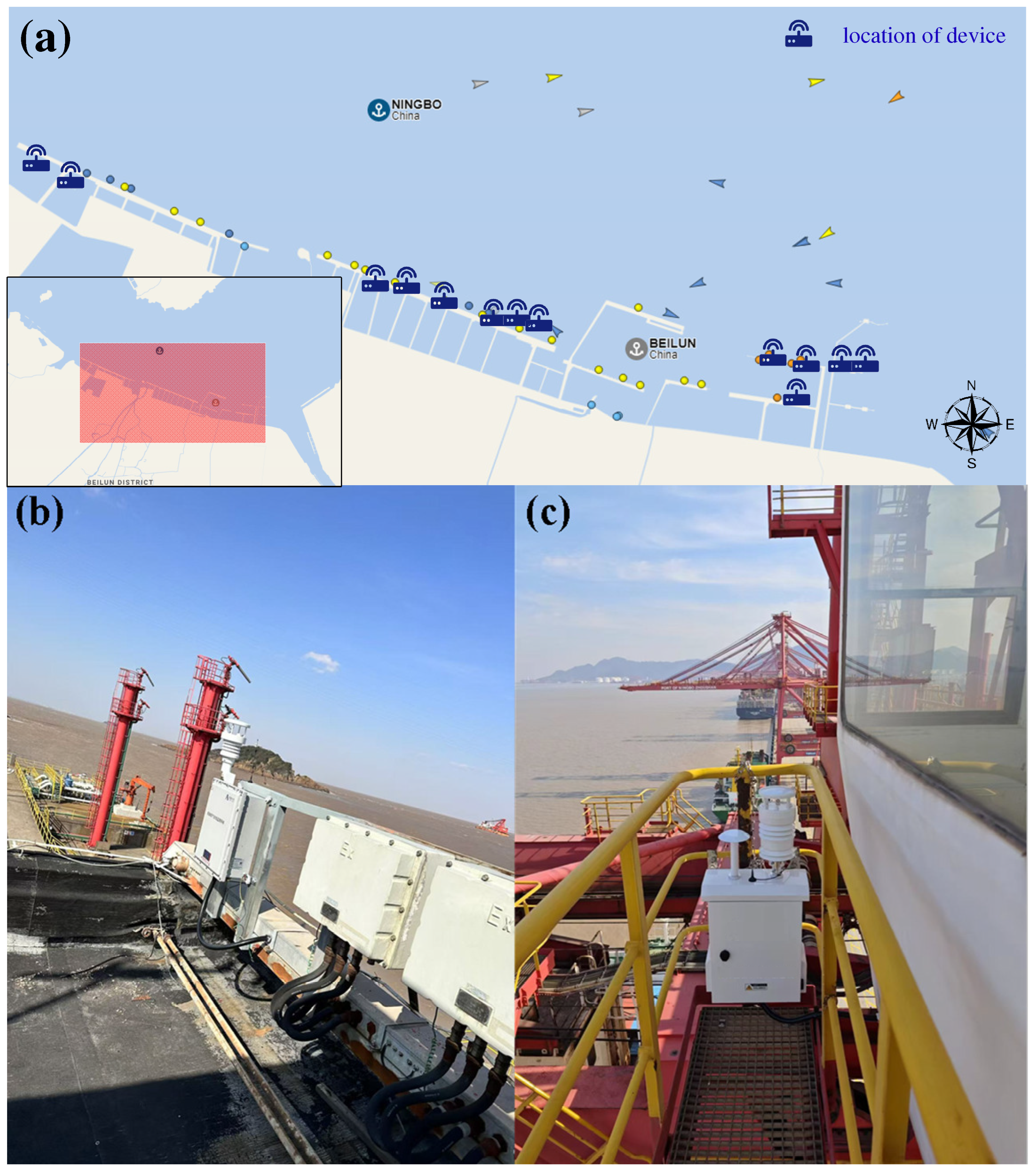
Ningbo Port is strategically located along the central section of China’s mainland coastline and serves as a significant coastal port within the southern wing of the “Yangtze River Economic Belt”. It functions as an essential hub in China’s national comprehensive transport system.
Figure 2a illustrates the installation locations of 13 monitoring devices, indicating that vessels may approach these monitoring sites. This suggests that the monitoring equipment operates within a complex environment designed to measure smoke plumes emitted by ships. The exhaust gas measurements collected at specific points may originate from multiple ship emission sources. Therefore, identifying potential emissions that exceed regulatory limits necessitates a comprehensive consideration of meteorological conditions, vessel information, and recorded gas values.
The installation positions on both the shore and bridge crane are depicted in
Figure 2b,c, respectively. In
Figure 2c, it can be observed that the left white antenna on the device is a GPS antenna; the small black antenna is designated for 5G connectivity; while the right component represents a compact weather station. When sensors detect concentration levels within the plume, these data are transmitted to a cloud computing centre via the 5G network. Notably, it was found that these installations were approximately 30–50 m from the berth, allowing for smoke plumes to disperse towards them after discharge.
Furthermore, since the equipment shown in
Figure 2b is fixed onshore and does not possess mobility features, it lacks a GPS antenna; however, its position was accurately measured during installation. Conversely, due to its mobility requirements, a GPS antenna has been integrated into the bridge crane illustrated in
Figure 2c.
The gas sensors of the sniffer equipment used to measure SO
2 and CO
2 were purchased from Shenzhen Singoan Electronic Technology Co., Ltd., Shenzhen, China (
https://www.singoan.com/ (accessed on 1 December 2018)). The SO
2 sensor was based on the electrochemical method and had a measuring range of 0–1 ppm, accuracy ≤ 10 ppb, resolution of 1 ppb, sampling rates 1 s, and a response time of ≤30 s. The CO
2 sensor was based on the nondispersive infrared analyser method and had a measuring range of 0–2000 ppm, accuracy of ≤5 ppm, resolution of 1 ppm, sampling rates 1 s, and a response time of ≤30 s. The instrument manufacturer provided these sensor characteristics, and calibration was used to ensure they were within the tolerances. Sensor calibration is required when the equipment is used daily and the time interval for sensor calibration is 3 months. The zero- and full-scales are usually calibrated by standard mixture gas. Standard mixed gases are usually “CO
2 + He” and “SO
2 + N
2”, with an accuracy < 3%.
2.2. Real-Time Detection
The data sources of ship FSC calculations were mainly collected using sniffer equipment and AIS antennas. These two data types are time-series stream data that require real-time reception and dynamic analyses. Therefore, this study selected the Redis memory database as the cache and used Spark Streaming for high-speed memory calculations (
Figure 3). After the sniffer equipment, AIS sent the data to the receiving end, and the interval (batch processing interval) was set so that the data were summarized to a certain degree and then operated together. The storage location was the Redis memory database. Via batch processing of exhaust gas concentration data, meteorological data, and AIS, it was determined whether the data of a time were suitable for the effective FSC calculation of ships. The determination rules included the following:
- (i).
Determine whether there is a ship target around the equipment according to the ship’s position from the AIS and the equipment’s position. The threshold value was set to 500 m according to experience.
- (ii).
Based on the positional relationship and meteorological data, determine whether the sniffer equipment is downwind of the ship target.
- (iii).
Determine whether there are gross errors in the tail gas concentration data or abnormal changes caused by equipment performance.
- (iv).
Confirm whether dynamic meteorological conditions, such as strong winds, rainfall, and turbulence, contribute to abnormal fluctuations in waste concentration data.
- (v).
Can a synchronized peak area of the SO2 and CO2 data be used for FSC calculation?
Then, according to the batch processing results, the measurement data that could be used for the effective FSC of the ship are sent to Spark Streaming to be decomposed into multiple Spark jobs. FSC calculations and object identification are performed in
Section 2.2,
Section 2.3 and
Section 2.4, respectively, and the acceptable ship target is finally obtained.
2.3. Background Value Recognition
After determining that the data in the cache could be used for FSC calculations, we further determined the background values using Equation (2). In some early studies, particularly those related to drones, the minimum measured value during the period before the measurement of the smoke plume was generally selected for FSC calculation. However, the sniffer monitoring equipment in the present study was in a complex dock environment, and the emission sources around the monitoring equipment (e.g., tugboats and container trucks) would have affected the background value, which is a dynamic changing process. According to Ausmeel et al. [
43], the contribution of ship emissions to the background value of a certain location in the dock area can be statistically calculated. Taking CO
2 as an example, the effect of ship emissions on the CO
2 concentration in the environment can be calculated as follows:
where CO
2,ship is the average CO
2 concentration emitted by a ship in a period; CO
2,bkg is the average background values of the selected period; n
ship,i is the number of passing ships during the selected period; t
plume,avg is the average duration of ship plume exposure; t
i is the period; and w
i is the proportion of time that the wind blows on the channel to the device location. Equation (2) can be used to calculate the average effect of ship emissions on the CO
2 concentration at the monitoring location. The background value fluctuated over time, as shown in
Figure 4. The measured CO
2 concentration emitted by the ship plume was calculated by subtracting the background value from the measured CO
2 concentration. Background SO
2 values were also determined in this manner.
2.4. Peak Region Recognition
After eliminating the effect of the background value, the measured value must be selected as the peak area for calculation, i.e., the integral interval in Equation (1) must be determined as the measurement values shown in
Figure 5a. In this study, based on experience [
27], we set the integral interval as the length of 10 data points and converted the sequence of measured values into the average sequence of 10 data points, as shown in Equation (3) and
Figure 5b. Thus, the selection of the integration interval in the gas-measured value series is transformed into the selection of the peak in the mean value series. Meanwhile, the implementation of this approach can also mitigate the effects of temporal discrepancies among sensors.
The numerator and denominator are divided by 10, where Avg(·) is the calculated function for the average measurement value within 10 consecutive data. Therefore, when the effect of R is ignored, the FSC calculation selects appropriate values for Avg(SO
2,peak), Avg(SO
2,bkg), Avg(CO
2,peak), and Avg(CO
2,bkg). Avg(SO
2,bkg) and Avg(CO
2,bkg) were calculated as described in
Section 2.2. Avg(SO
2,peak) and Avg(CO
2,peak) were positioned using second-order difference operations after converting to first difference (
Figure 5c), as shown in Equation (4) [
23].
C(t) represents the measured CO
2 concentration at time t. Using Equation (4), we can determine the peak point of the mean value series as shown in
Figure 5d. Because the time series is discrete, multiple alternative peaks of CO
2 can be obtained after setting the threshold close to zero. Similarly, SO
2 produced an alternative peak. Finally, a pair of Avg(SO
2,
peak) and Avg(CO
2,peak) was selected for the calculation of Equation (3), with the minimum time interval as the screening condition.
In addition, this avoided the effect of environmental factors or sensor jump data on the monitoring results. The time point of an abrupt change in the measurement data can be selected based on the results of the first-order difference operation, and the corresponding measurement values can be deleted. The above peak-region filtering process is illustrated in
Figure 5. It should be added that the measured values at this time already represent the SO
2 and CO
2 concentrations provided by a particular emission source, which means that interference from other sources is eliminated as much as possible, and cross-interference such as NO
2 sensors is corrected, which will be discussed in more detail in the uncertainty analysis. In addition, the response time of different sensors is different. We receive the measured values of all sensors at a frequency of 1 s at the receiving end and store them in the cache or database.
2.5. Emission Source Locking
Because of the complexity of the monitoring environment, multiple ship targets might be located around the sniffer equipment at the same time. The FSC calculated in
Section 2.4 was derived from the measurements taken by the sniffer equipment, and it was impossible to directly distinguish from which ship the detected plume was emitted. In this study, in addition to obtaining gas concentration information, the sniffer equipment was also equipped with sensors for wind speed, wind direction, air pressure, humidity, and pressure, which could obtain real-time meteorological information around the equipment. Simultaneously, maritime mobile service identification from AIS can be associated with ship power databases to obtain technical parameters, such as engine power. Based on these data, a Gaussian plume model was used to identify the emission sources.
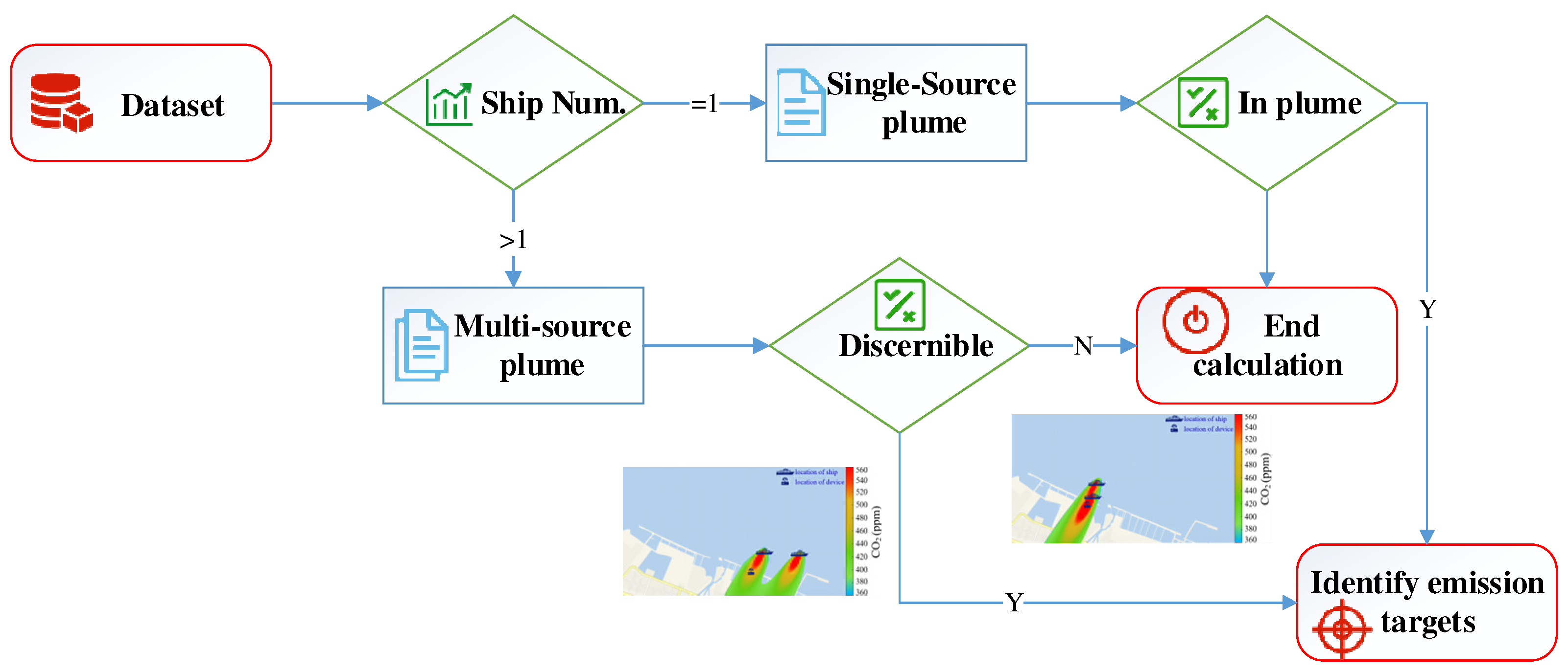
The process illustrated in
Figure 6 was designed to identify the discharge ships. A batch dataset was obtained based on the procedures described in
Section 2.2,
Section 2.3 and
Section 2.4, and a single/multiple-plume simulation model were then generated according to the number of ships around the equipment (note: distance from the ship was <500 m; this means that only ships within a 500 m radius around the equipment are considered as potential FSC estimation targets, not that emissions from ships beyond 500 m will not be detected or have no impact). If the number of ships was 1, it was further determined whether the sniffer equipment was within the plume. If the number of ships was >1, the emission values contributed by different ship targets in the equipment space could be simulated according to the smoke plume model, and the differences in the simulated values of different ships could be used to determine whether the main emission targets were sufficiently identified.
According to Jalkanen [
44], The smoke plume simulation method based on the Gaussian model is shown in Equation (5):
where C(x,y,z) is the gas concentration (CO
2 in the current study) at any point in the environment; Q is the strength of the point source (i.e., the emission rate of the gases in kg/s), which can be utilized to calculate the assessment model of ship traffic emissions; H is the effective chimney height that involves the actual chimney height plus the puff rise height. The puff rise height is calculated using the method proposed by Peng et al. [
30]. The actual chimney height is determined based on an empirical value set by the ship’s length. Specifically, when the ship’s length is greater than or equal to 30 m, the chimney height is not less than one-tenth of the ship’s length, and the minimum height is not less than 6 m. When the ship’s length is less than 30 m, the chimney height is not less than one-fifth of the ship’s length, and the minimum height is not less than 4 m;
and
are dispersion coefficients in the y and z directions, respectively, which depend on atmospheric stability; and u is wind speed, which was measured by the sniffer equipment.
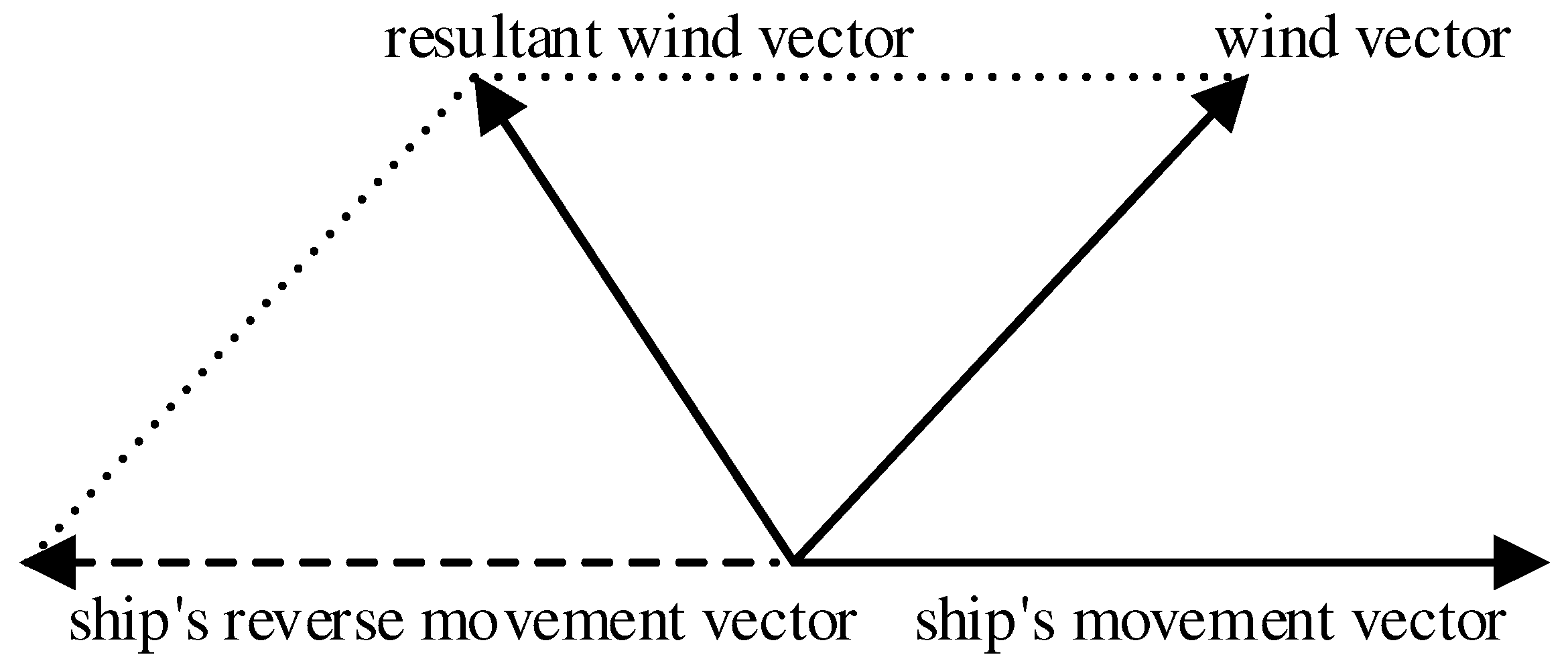
The classical Gaussian plume model does not consider the influence of the target ship’s movement; hence, the wind speed and direction from weather data could not be used directly.
Figure 7 shows that the ship’s movement vector and wind vector were generated at a certain angle to produce the ship’s reverse movement vector. The resultant wind vector is then obtained according to the rules of vector synthesis. If wind speed and direction are variable, the cloud computing centre can re-calculate the position of the ship’s plume every time it receives AIS information.
As shown in
Figure 6, when multiple ship targets contributed to the gas concentration in the monitoring equipment, it was necessary to distinguish them further based on the simulation results of the Gaussian plume. Based on the AIS information of different ships, their speed and course of navigation can be obtained. The resultant wind vector of each plume can be calculated by combining the measured wind speed and direction obtained from the sniffer equipment, thereby calculating the gas concentration contribution value of the ship’s plume to the measurement position according to Equation (5).
In this research, when a peak area is detected at a certain time point through
Section 2.2,
Section 2.3 and
Section 2.4, the FSC result can be calculated. Based on AIS information, more detailed engine parameters of the sniffer equipment’s surrounding ships are obtained to estimate the emission intensity of each target ship. Then, using Equation (5) and the local meteorological information measured by the equipment, the CO
2 gas concentration value at the sniffer equipment location due to the emissions from surrounding ships is estimated. When two or more plumes overlap at the sniffer equipment location, the maximum value is selected and compared with the other values. If the proportion of the other values does not exceed 5% of the maximum value [
44], it is considered that the value corresponding to the target ship can be ignored. Otherwise, it is considered that with the measurement data, it is difficult to pinpoint specific emission targets.
However, this method is based solely on the CO
2 estimated value of different ships. If two ships use fuels with different FSCs, the influence of the smaller CO
2 estimate value for one ship may be only 5% [
44], but would be significantly higher for SO
2 emissions. In this case, the true FSC values for different ships are impossible to estimate. This is especially the case for when the plumes of ships at berth (auxiliary engine as main emitter) are mixed with plumes from sailing ships (main engine as main emitter). Therefore, if the calculated FSC value exceeds the upper limit value, all unignorable targets are listed as potential over-limit objects, and the FSC results are temporarily assigned to these objects for subsequent verification.
2.6. Uncertainty Analysis
The uncertainty associated with FSC measurement encompasses various factors, including calculation uncertainty, emission uncertainty, gas distribution uncertainty, gas calibration uncertainty, and cross-interference uncertainty [
45]. The overall FSC uncertainty (
) can be represented by the following formula:
indicates computational uncertainty. According to Formula (3), selecting different peak and background values from the monitoring data segment during calculations can lead to deviations in the results. For SO2 and CO2, various potential peak and background values are considered sequentially, and these are compared with the measured FSC. The cumulative sum of all calculation deviations constitutes the overall computational uncertainty.
represents emission uncertainty, which arises because approximately 1% to 19% of sulphur in fuel is not fully converted into SO
2 [
46]. In this analysis, it is assumed that all sulphur present in the fuel is completely transformed into SO
2. Based on research conducted by Schlager et al. [
46], a measured FSC value of 15% is utilized to denote the uncertainty associated with individual emissions.
indicates the uncertainty in gas distribution, which is influenced by factors such as temperature and humidity, leading to a non-uniform distribution of gas within the sensor. Based on the research conducted by Mellqvist et al. [
45], we utilize 10% of the estimated FSC to represent the uncertainty associated with gas emissions.
and denote uncertainties arising from monitoring errors related to sensor calibration for two different gases. A third party evaluated the accuracy of our equipment’s gas measurements. The report indicates that the monitoring errors for SO2 and CO2 are 0.033 and 0.021, respectively.
represents cross-interference uncertainty; when sulphur oxides are discharged from a ship, nitrogen oxides may also be released into the sniffer, resulting in SO
2 exhibiting a certain degree of cross-sensitivity to NO. Therefore, it is essential to calibrate the SO
2 monitoring values against those measured for NO [
24]. According to Balzani Lööv et al., 15% of the measured FSC is employed to account for uncertainties due to single cross disturbances.
3. Experiment, Results, and Application
Based on previous studies [
23,
27,
32], we developed a continuous, low-cost, and low-power ship plume measurement system utilizing the architecture illustrated in
Figure 1. We analyzed and processed the real-time data collected by this equipment according to the analytical methods outlined in
Section 2.2,
Section 2.3,
Section 2.4 and
Section 2.5. By obtaining real-time measurements of FSC, this system is capable of providing rapid warning services for the maritime sector. In 2023, we installed this system at Ningbo Port, China, to estimate ship FSC based on measured gas concentrations. This estimation was then compared with true FSC values obtained by the maritime department during onboard inspections when oil samples were extracted, thereby verifying the practicality and effectiveness of the proposed method.
3.1. Typical Plume Data
To elucidate the calculation process of this analysis, we selected representative cases from the acquired dataset for detailed examination and explanation, as illustrated in
Figure 8a. This figure presents plume measurement data exhibiting a distinct peak value, which facilitates the calculation of the ship’s FSC. While other peak regions are evident at marked points, we opted to select the largest peak region as the calculated FSC value. This choice is predicated on the premise that a larger peak signifies a higher concentration of ship emissions in the atmosphere, thereby minimizing interference from environmental noise.
The measurement data depicted in
Figure 8b demonstrated an abrupt change; specifically, the SO
2 measurement increased from 0.01 ppm to 0.5 ppm. Such fluctuations may have resulted from either an anomalous sensor or turbulence disturbances within the environment. Additionally, there were instances of noise present in CO
2 measurements (with wave peaks exceeding 500 ppm). Consequently, these measured data could not be utilized for calculating FSC values; thus, we omitted the research methodology outlined in
Section 2.2.
Figure 8c illustrates a plume characterized by an unsynchronized peak value with SO
2 measurements fluctuating between approximately 0.008 and 0.012 ppm (indicating both low magnitude and minimal variation). The data obtained under these conditions may have been influenced by external sources of interference; for instance, when a truck passed near monitoring equipment using diesel fuel with sulphur content < 0.001% (m/m), its emitted SO
2 was negligible while CO
2 emissions remained measurable by our apparatus.
Such data were excluded from consideration during peak identification as described in
Section 2.2 and could not contribute to FSC calculations either. Although multiple simultaneous peaks of CO
2 and SO
2 appeared (as shown in
Figure 8d), significant discrepancies arose when calculating FSCs based on different peaks—likely due to monitoring equipment capturing gas emissions from several disparate sources during this timeframe.
This condition was identified and subsequently excluded following protocols delineated in
Section 2.5. Additionally, it should be noted that the peaks identified in
Figure 8 are the peaks in the mean value series, which are equivalent to the integral value within a 10 s period, according to Equation (3).
3.2. FSC Comparison Verification
From June to August 2023, we jointly verified the practical effect of this system with the maritime department, i.e., maritime law enforcement officers boarded the ship to extract fuel samples, sent them to a third-party laboratory for inspection to obtain the true value of the FSC of the ship, and compared it to the FSC estimated using this method. Eight ships were monitored (
Table 1).
Indeed, in validating with eight samples is difficult to effectively prove the accuracy and effectiveness of the proposed method from a statistical perspective. However, in the process of measuring actual ship plumes, the opportunity to conduct onboard inspection is extremely limited. This is not limited to our research, but to all ship exhaust emission measurement activities, because it requires the maritime authorities to carry out inspection within the limits of relevant regulations. The research team cannot independently decide the number and target of ships for onboard inspection, and these results were learned from the maritime authorities within the measurement period. In any case, this can to some extent demonstrate the effectiveness of our method.
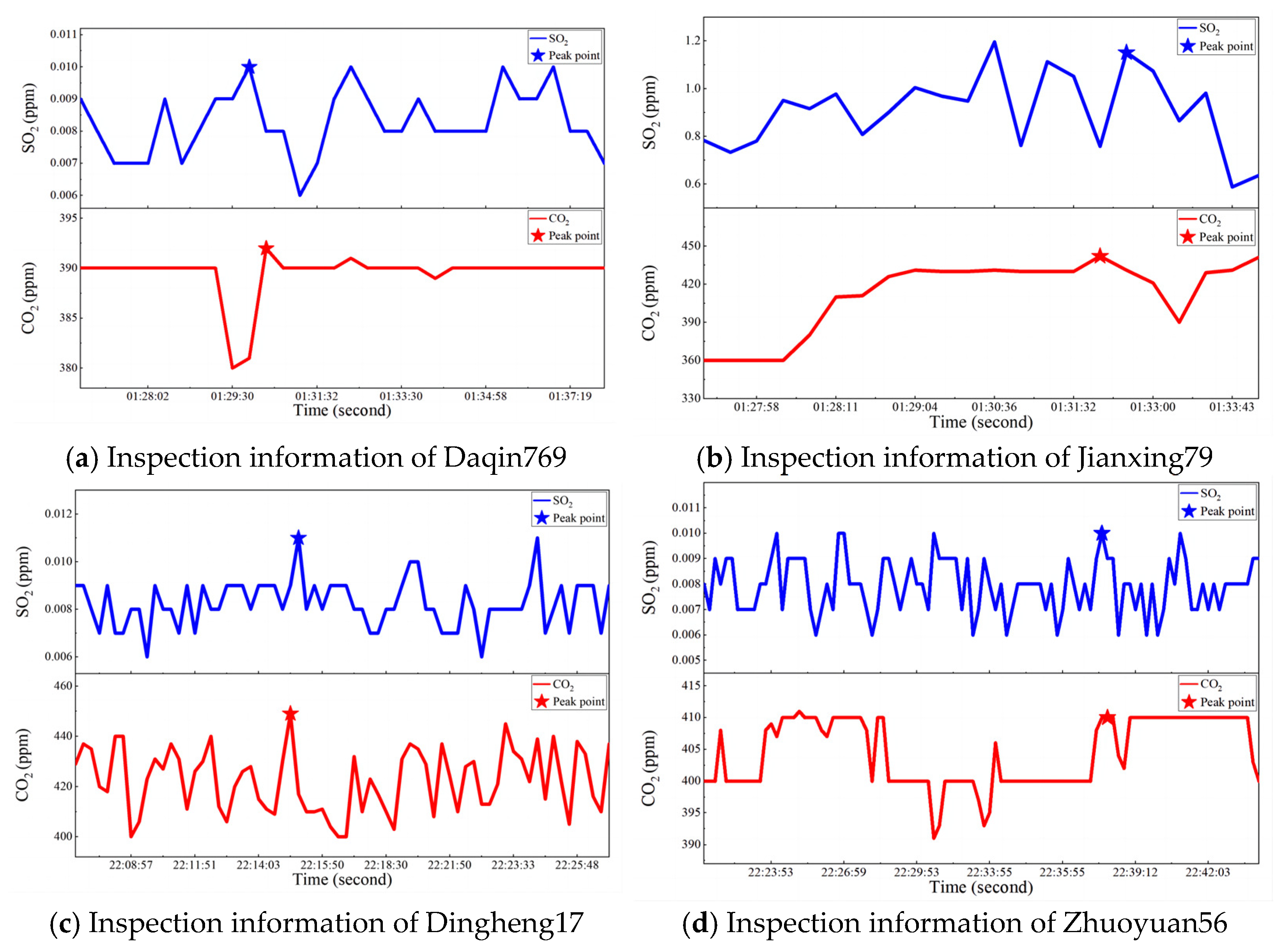
The accuracy of the Fuel Sulphur Content (FSC) calculation results at the 0.10% (m/m) and 0.50% (m/m) levels is critically important. These two values represent the upper limits of the relevant FSC restriction policy, serving as the sole indicators for determining compliance of fuel oil used by ships. Consequently, measurement accuracy at these levels directly influences the practicality of the monitoring system. As illustrated in
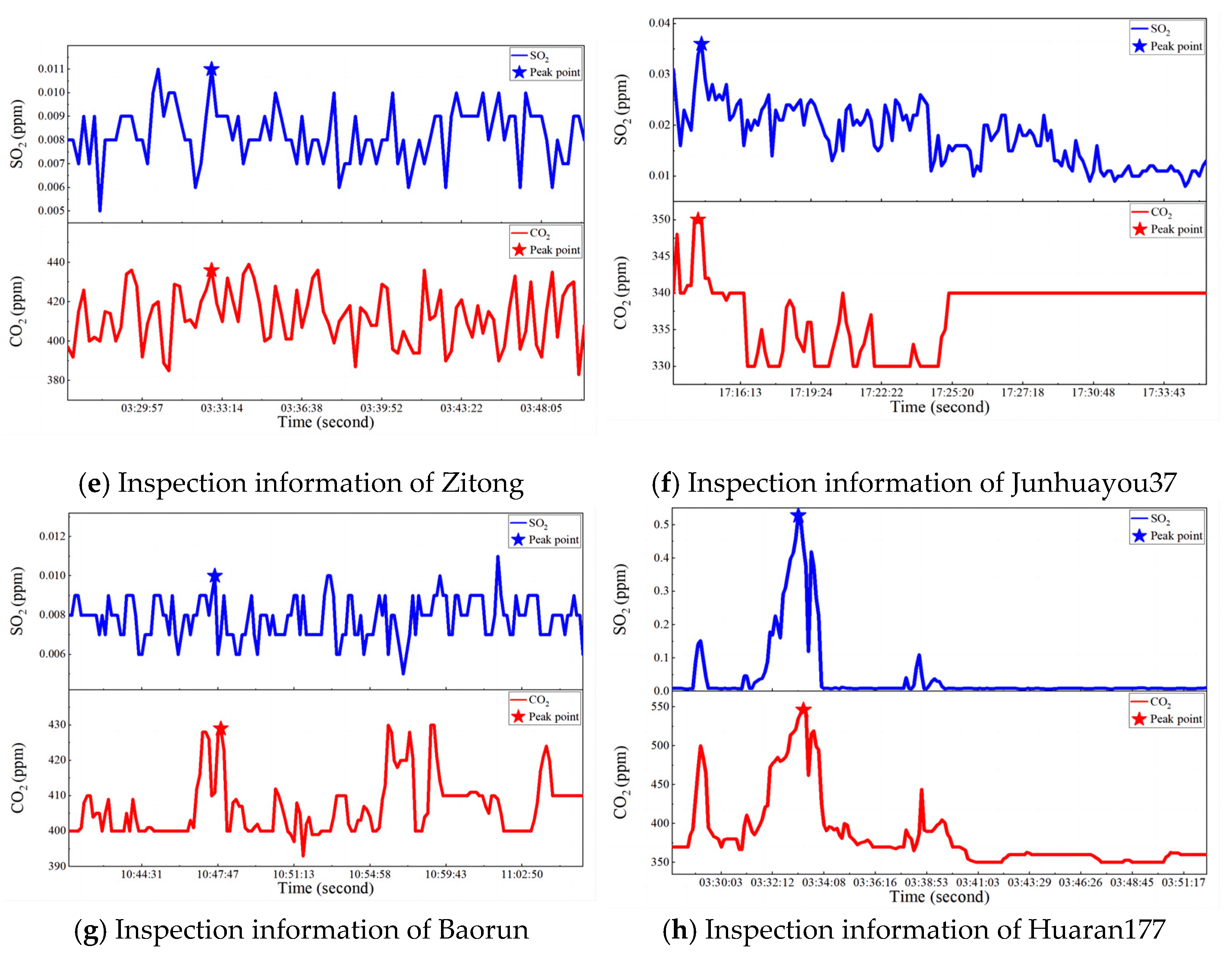
Table 1, seven ships exhibited an FSC < 0.10% (m/m), with measurements obtained from the sniffer monitoring system also indicating values below this threshold, thereby confirming that this system can accurately measure FSC at this level. It is noteworthy that measurement difficulty escalates as FSC levels decrease; thus, relative deviation tends to increase due to sensor performance limitations and environmental interferences. For instance, relative deviations observed in cases No. (a) and (f) were more pronounced; however, these calculations were derived from an FSC level of 0.01% (m/m), where the absolute value of deviation was approximately 0.06% (m/m). The measured values corresponding to these ships’ target plumes are presented in
Figure A1.
Measurement uncertainty has been calculated individually for each assessment conducted on these vessels. The average value of FSC uncertainty across these seven ships was determined to be 0.0505% (m/m). Results indicate that actual FSC values for these vessels fall within our estimated range. One ship recorded an actual FSC value of 0.498% (m/m)—very close to the upper limit of 0.50% (m/m)—while readings from sniffer monitoring equipment indicated a value of 0.5399% (m/m). Although there was some degree of deviation noted between these measurements, it remained relatively minor.
According to previous studies, deviations measured using Uncrewed Aerial Vehicles near a ship’s chimney typically remain below <0.03% (m/m) [
27,
28,
29]. The sniffer equipment utilized in this study was land-based, positioned at a considerable distance from the ship’s chimney. The resulting deviation measured 0.0419% (m/m), which is relatively significant. Overall, the deviation observed with the land-based sniffer method exceeds that of the UAV sniffer method. This finding is logical, as land-based sniffers are situated farther from ship chimneys and are more vulnerable to environmental interference. Nevertheless, they can serve an effective early warning function in practical applications.
This is because onboard inspections are carried out by the maritime authorities, of course, and they must follow certain regulatory and legal procedures. As a research team, we cannot independently decide the number and target of ships for fuel sampling on board. The number and target of onboard inspections and fuel sampling that I have learned from the maritime authorities within the measurement period include only the eight ships mentioned above.
3.3. FSC Data Statistics
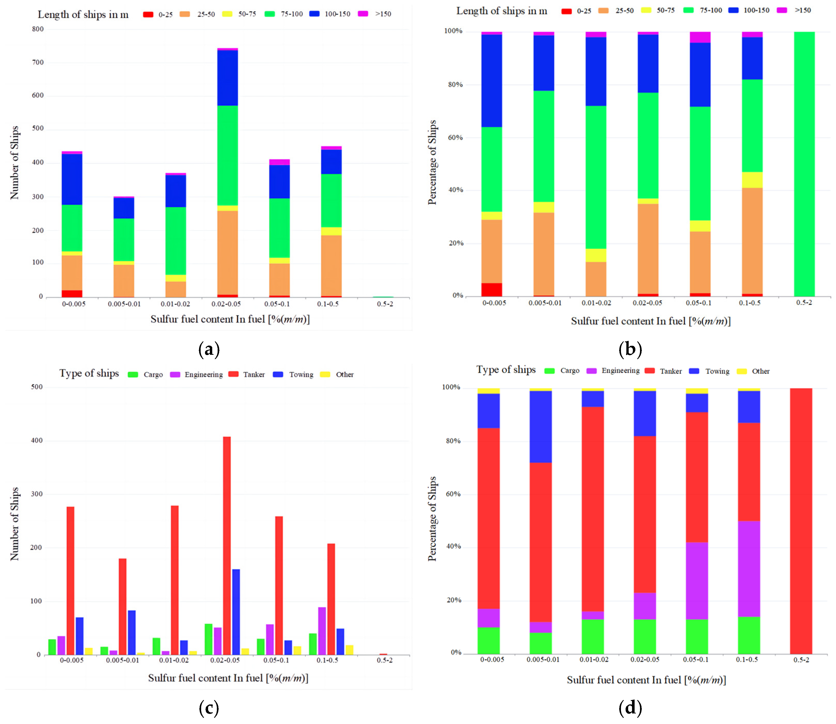
Between June and July 2023, the sniffer monitoring network deployed in the Ningbo Port area effectively monitored 2624 ship objects cumulatively. The FSC distribution was statistically analyzed according to the ship length and type, as shown in
Figure 9.
The FSC of the majority of ships was found to be less than 0.50% (m/m), with most values distributed within the range of 0.02–0.05% (m/m). Only a limited number of vessels exceeded the upper limit of 0.50% (m/m). Notably, those ships that surpassed this threshold were predominantly in the length category of 75–100 m, accounting for all instances; however, this group comprised only five vessels in total, which is insufficient to conclusively demonstrate a high violation rate among small seagoing ships. Furthermore, as illustrated in
Figure 9c,d, the primary types of ships monitored during this study were tankers, followed by towing vessels. The few ships exceeding the upper limit of 0.50% (m/m) were also identified as tankers. This observation can be attributed to our monitoring equipment being deployed at liquid cargo terminals where tankers and tugboats are primarily active.
Overall, it can be concluded that most targeted vessels within this region adhered to the ECA’s FSC limit set at ≤0.50% (m/m), with very few exceptions noted among those measuring between 75–100 m in length—specifically small seagoing ships. A significant concern arises from over 400 vessels whose FSC ranged between 0.10–0.50% (m/m). With China’s implementation of its ECA policy on the horizon, it is anticipated that adjustments will soon align the FSC limit to approximately 0.10% (m/m) for consistency with current regulations established by IMO regarding FSC limits. These seagoing vessels constituted roughly 15%, while their respective FSC levels remained below <0.10% (m/m). However, it should be noted that implementing maritime sector policies may encounter certain initial challenges.
3.4. Application Effect
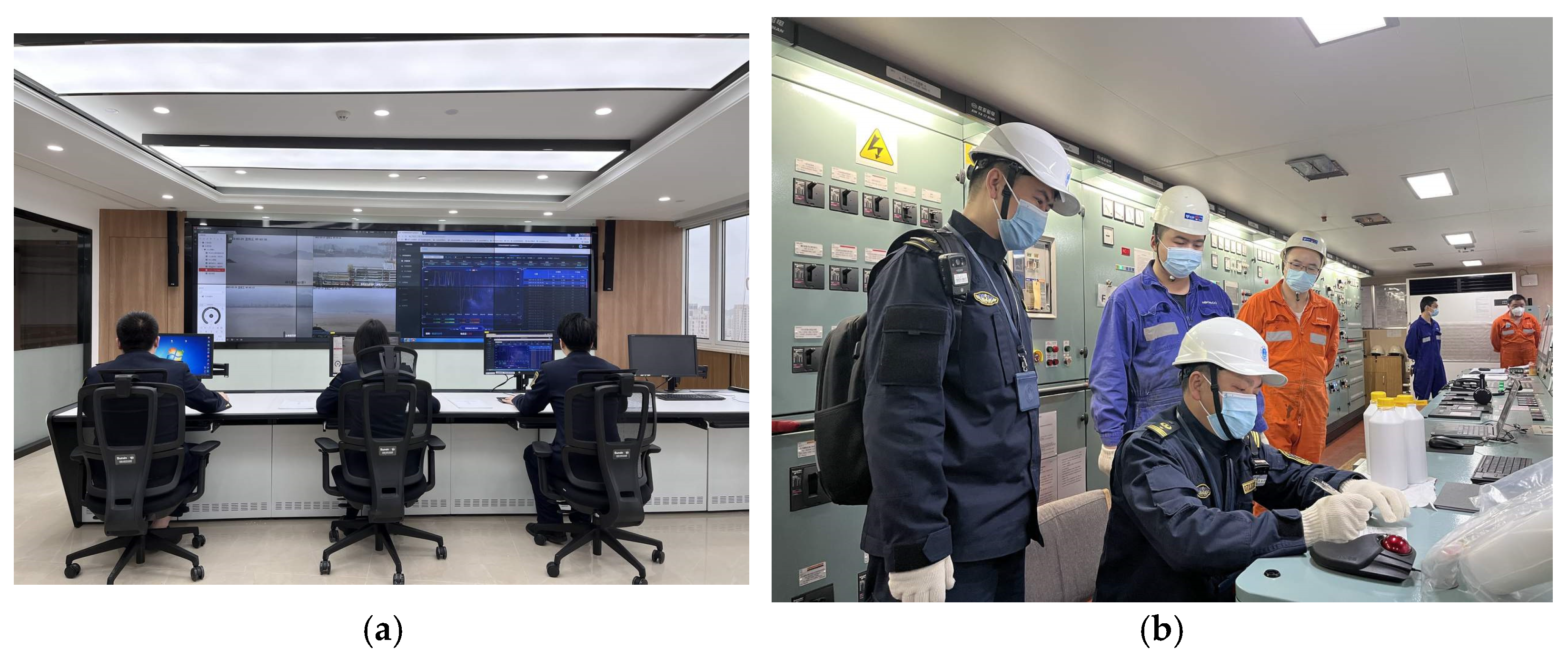
Since the system was implemented in Ningbo Port, the law enforcement efficiency of maritime personnel has significantly improved. As shown in
Figure A2a, supervisors can remotely monitor the real-time situation of ship emissions at the traffic command centre and screen suspicious ship targets according to the FSC calculated by the system. Subsequently, the supervisor boards the ship to inspect the ship fuel sample extraction, as shown in
Figure A2b. This method overcomes the disadvantages of random and uncertain ship target monitoring, significantly improving the efficiency and effectiveness of ship FSC monitoring.
In addition, our monitoring system is 7 × 24 h. Once the FSC of a ship is found to exceed the limit, it will immediately send a system notification and a short message service (SMS) or email for alarm. However, the timing of the alarm may not be appropriate for maritime authorities to arrange for the appropriate personnel to board the ship. Therefore, the maritime authorities have listed it as a priority object of observation and may arrange to board the ship for inspection at an appropriate time, or the ship may be reported to the inspectors as the next port of call for a follow up inspection.
4. Conclusions
Analyzing ship smoke plumes and calculating ship FSCs using the sniffer method is an effective ship emission control measure. However, simultaneous emissions of plumes from multiple ships and other combustion emission sources (trucks, power supply units, …) in busy dock areas pose a challenge in calculating the ship’s FSC. To address the difficulty in measuring FSC in complex port environments, a ship emission monitoring system and an FSC calculation model are proposed in this study. Using real-time monitoring, background value identification, peak value identification, and emission source contraction points, the FSC of ship targets can be effectively monitored, and the law enforcement efficiency of maritime supervision can be improved.
We conducted a field observation campaign at Ningbo Port in China and cumulatively measured 2624 ships between June and August 2023. We randomly selected eight ships to verify the accuracy of the FSC measurements, and the results showed that the system achieved accurate FSC measurements at 0.10% (m/m) and 0.50% (m/m) levels. In addition, we conducted uncertainty calculations on the FSC calculation of these ships, and the results prove the reliability of our FSC calculation method. Statistical analysis of the FSC of 2624 vessels showed a greater proportion of small seagoing vessels in the terminal area with FSCs, which may have exceeded the standard. In addition, with approximately 15% of ships using fuel oil with FSC > 0.10% (m/m), there may be future challenges in implementing more stringent FSC limits.
This study presents an efficient and remote detection method for land-based sniffing of FSC, aimed at enhancing law enforcement efficiency while minimizing the human, financial, and temporal costs incurred by maritime authorities. This approach is particularly significant in deterring the illegal use of high-sulphur ship fuels and improving air quality in port areas.
In future research, we will continue to test and optimize our methodology across various detection environments. Furthermore, we plan to incorporate additional factors such as sulphide deposition and sensor cross-sensitivity into the computational model to further enhance the accuracy of monitoring results.


