1. Introduction
Wave measurement is vital for understanding oceanic processes and managing the marine environment [
1,
2,
3,
4,
5]. It contributes to energy transfer in the ocean, affects current formation and plays a key role in sediment transport and shoreline morphology. Accurate wave data are essential for monitoring and predicting coastal erosion, sea-level rise and the broader impacts of climate change. In addition to their environmental relevance, wave conditions have practical implications for maritime safety, navigation, offshore operations and recreational activities. From supporting storm surge forecasting to informing the design of coastal defences, reliable wave monitoring is vital for protecting both human infrastructure and natural ecosystems.
Waves are generated by wind transferring energy to the ocean surface, underwater seismic activity and gravitational effects from celestial bodies [
6]. Once formed, waves may travel long distances as swells, which persist even after the wind subsides and can impact coastlines far from their origin [
7]. As waves approach shorelines, decreasing depth causes them to slow, grow in height and break, releasing energy.
To effectively analyse and communicate wave conditions, a clear understanding of the standard terminology is essential [
8,
9,
10]:
Wave height refers to the vertical distance between a wave’s crest (highest point) and the trough (lowest point).
Wave period is the time interval between successive wave crests passing a fixed point.
Wavelength is the horizontal distance between two successive wave crests.
Significant wave height is a statistical measure representing the average height of the highest one-third of waves in a given dataset.
The analysis of wave conditions depends on a combination of the previously mentioned parameters. The most evaluated metrics for assessing wave conditions are wave height and wave period, which are the primary indicators of wave energy and overall sea state.
Traditional wave monitoring technologies have been foundational in advancing our understanding of wave dynamics and remain integral to both research and practical applications. These technologies are essential for measuring key wave characteristics, such as height, period and direction, which are critical for various applications. Among the most recognised tools for wave measurement are wave buoys, which can be equipped with accelerometers, gyroscopes, wave gauges and global positioning systems (GPS) [
11,
12,
13]. These floating devices measure the vertical acceleration of the water surface, converting it into wave height data. The system also calculates wave direction and period by tracking the buoy’s motion. Some buoy designs can also employ acoustic technology, offering alternative methods for wave monitoring [
14]. Despite their widespread use, wave buoys come with certain limitations. They are expensive to deploy and maintain, and their fixed positions provide data only from specific locations.
Pressure sensors are another traditional technology used for monitoring waves, usually deployed on the seafloor or underwater platforms [
15,
16]. These sensors measure the pressure exerted by the overlying water column, which varies with wave motion. One can infer wave characteristics such as height and frequency by analysing these pressure fluctuations. Like wave buoys, pressure sensors are stationary and provide data from specific locations, limiting spatial coverage. Moreover, the absolute pressure due to the water column is higher at greater depths than at shallower depths, causing the relative pressure changes from waves to become smaller. As a result, detecting small wave-induced pressure changes becomes more challenging. This means that pressure sensors need to be calibrated for their deployment depth, and there is a correlation between the depth of installation and the resolution of wave measurements.
Remote-sensing technologies offer a valuable alternative to direct contact sensors for monitoring sea waves without physical interaction with the water surface and providing broader spatial coverage and timely insights. These methods include satellite-based systems [
17,
18,
19], cameras [
20,
21], light detection and ranging (LIDAR) [
22], radar technologies such as high-frequency (HF) radar and X-band marine radar [
23,
24], and seismometers [
25,
26]. Satellite systems provide extensive global coverage and can track large-scale phenomena, but they are limited by factors such as temporal resolution and cloud cover. Cameras, including those used for optical imaging and photogrammetry, can capture wave characteristics and patterns, though their effectiveness is influenced by lighting and weather conditions. LIDAR offers high precision and rapid data collection from airborne platforms, though its effectiveness may diminish in rough conditions. HF and X-band radar systems excel at real-time monitoring of surface waves and currents over coastal regions, but environmental factors and land interference can constrain their range. Seismometers complement these technologies by detecting microseisms generated by ocean waves, but their effectiveness is limited by the indirect nature of the measurements and potential interference from other sources of ground vibrations.
As the demand for comprehensive and real-time ocean monitoring grows, the limitations of traditional wave measurement technologies become increasingly evident. Addressing the complexities of marine environments calls for more resilient and efficient monitoring solutions. In this context, marine fibre optic cables have emerged as a promising technology, offering a novel approach to wave monitoring that can significantly enhance data collection capabilities. In fact, sensing along the marine cable length has been explored previously in the context of wave monitoring [
27,
28].
Marine fibre optic cables are extensive networks that traverse vast oceanic regions, installed initially for telecommunications purposes. One of the most compelling advantages of using marine fibre optics is the ability to leverage an extensive, pre-existing network of submarine cables. These cables traverse large portions of the ocean, including remote and deep-sea areas that are often difficult to monitor with conventional equipment, such as buoys and radar systems. Combined with advanced monitoring technologies, marine fibre optic cables offer the potential for real-time data transmission and high-precision wave measurements across different regions [
29,
30,
31]. These cables can support various sensors—from pressure sensors to other acoustic and environmental sensors—that can capture detailed information about wave height, period, direction and energy. The ability to transmit data in real time is a critical advantage, especially for applications requiring immediate responses, such as tsunami warning systems and maritime safety operations. This real-time capability allows for the prompt dissemination of information, which is crucial for decision making in dynamic and potentially hazardous environments.
As new submarine cables are laid to support growing global communications needs, there is an opportunity to design these networks with integrated monitoring technologies from the outset. This forward-looking approach allows for the scalability of monitoring efforts, enabling the expansion of monitoring capabilities in parallel with the growth of global telecommunications infrastructure. Additionally, the ability to retrofit existing cables with advanced sensors provides flexibility and adaptability, ensuring that current networks can be upgraded to support emerging monitoring needs.
This study investigates the integration of pressure sensors into a 2000 m marine cable demonstrator, deployed off the Portuguese coast as part of the Knowledge and Data from the Deep to Space (K2D) Project, to enable real-time monitoring of tidal cycles and sea wave characteristics. By developing and validating a methodology to estimate sea wave height and period at multiple depths using pressure-based measurements on the seafloor, this work advances environmental measuring technology and explores the feasibility of repurposing existing undersea infrastructure for oceanographic sensing. The results provide a valuable proof of concept for low-cost, scalable and real-time monitoring systems that can be extended to broader sensor networks for marine and climate research.
2. Materials and Methods
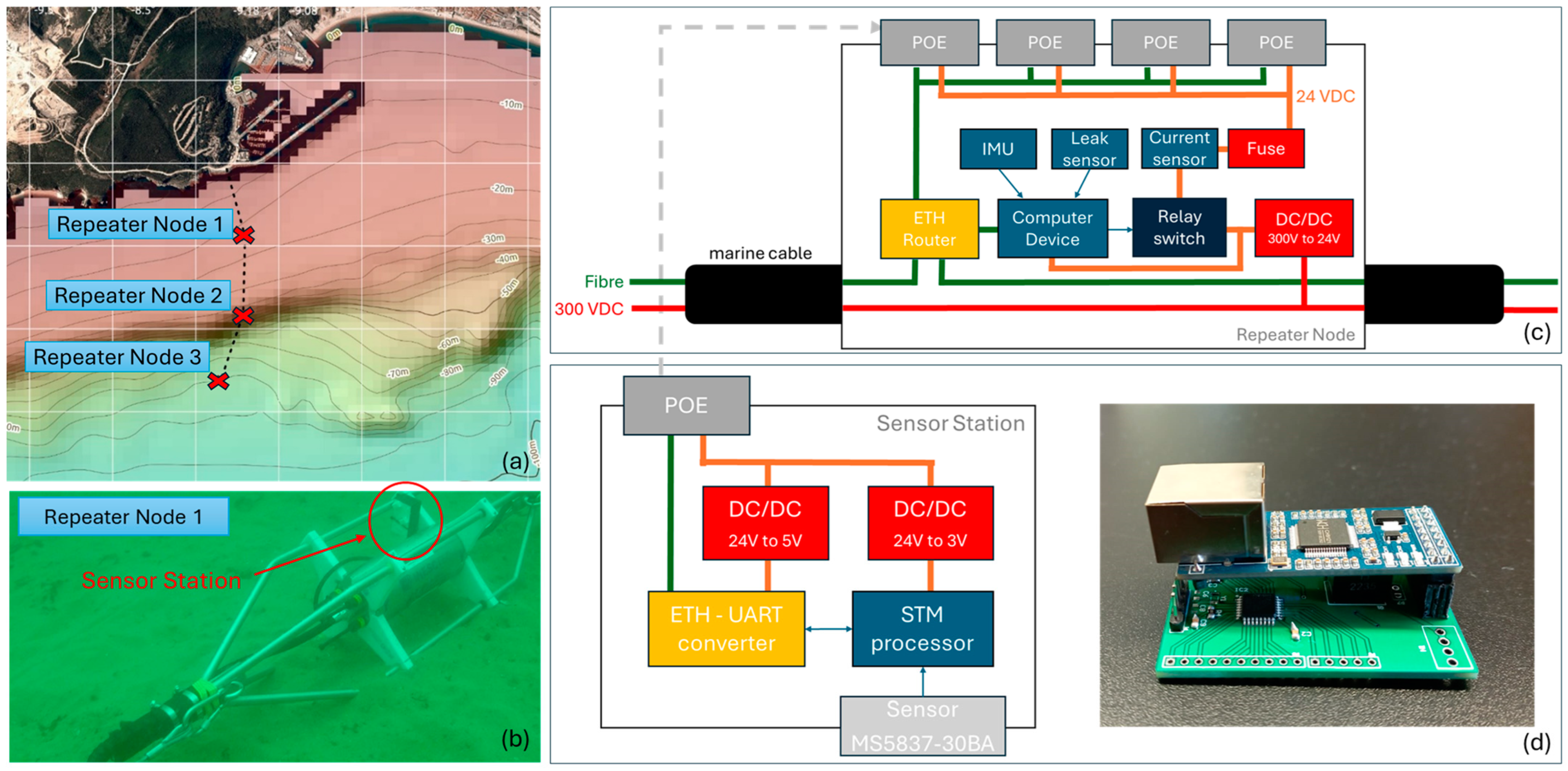
The K2D Project is a collaborative initiative between several Portuguese institutions and the Massachusetts Institute of Technology (MIT) in the USA. The project aimed to enhance the functionality of smart cables by expanding their measurement capabilities, integrating active devices and leveraging moving platforms like deep-sea autonomous underwater vehicles (AUVs) to increase the spatial coverage of measurements along the cables. In this innovative approach, each repeater serves as a hub for additional equipment, such as active devices, sensors to monitor physical, chemical and biological variables, docking stations for AUV battery charging and data exchange and acoustic beacons for AUV navigation. The K2D Project aimed to take the initial steps towards demonstrating this new vision of smart repeaters as hubs for local observatories and AUV interactions. To test and validate this concept, a wet demonstrator was designed and deployed in the summer of 2023 off the coast of Sesimbra, Portugal (38°25′59.6″ N 9°06′56.0″ W), with the support of the Portuguese Navy vessel NRP Andrómeda [
32,
33]. Considering the resources available in the K2D Project and its demonstration objectives, the final design involved the deployment of a 2000 m cable, which included three repeater nodes, each one comprising a sensor station to monitor sea waves.
2.1. Repeater Nodes and Sensor Station Design
Three repeater nodes were prepared for this demonstration, all similar in composition, with the only difference in the last node, which did not have an exit gland. The housings were designed to withstand pressures up to 120 bar (1200 m) and mechanical traction of up to 104 Newtons. To reduce the energy loss, the cable was powered with 300 volts direct current (VDC). Each of the three repeater nodes featured a sensor station, which served as a terminal for aggregating sensor data and transmitting them via the Ethernet backbone. These stations could accommodate a variety of underwater sensors, boasting advanced capabilities in signal acquisition, data processing, memory and communication.
For this study, the three sensor stations were equipped with MS5837-30BA sensors to measure water temperature (from −20 to 85 °C with 0.1 °C resolution) and pressure (0–30 bar with 0.2 mbar resolution). This low-cost and low-power sensor has been tested in previous coastal monitoring studies [
34]. The sensor stations of repeater nodes 1 and 2 were configured to provide water temperature and pressure data with a sampling period of 300 ms, and the sensor station of repeater node 3 was configured to provide these data with a sampling period of 1 s.
Each station was built with a printed circuit board that housed an STM32L056C6T6 processor, a universal asynchronous receiver/transmitter (UART) to the Ethernet converter and power circuits. The processor managed the sensing devices and utilised the UART channel to transmit the monitoring data to the converter, which then fed them into the Ethernet bus via a power over Ethernet (PoE) connector. The electronics were encapsulated in polyurethane resin to ensure the system met watertight requirements.
Figure 1 illustrates the installation of the fibre optic cable, an underwater photograph of one of the repeater nodes, the electric design of the repeater nodes and the design and printed circuit board (PCB) layout of the sensor stations.
2.2. Conversion of Data Pressure to Depth
The three sensor stations were equipped with MS5837-30BA sensors that measure absolute pressure in millibars (mbar). Absolute pressure includes both the atmospheric pressure at the surface and the pressure exerted by the water column above the sensor. To determine the depth of the water (or height of the water column) based on this reading, the following formula is applied:
where
d = depth [m];
P = pressure measured by the sensor [bar];
P0 = atmospheric pressure (1 bar);
ρ = seawater density (1025 kg/m3);
g = gravitational acceleration (9.81 m/s2).
This formula calculates the height of the water column above the sensor by subtracting the atmospheric pressure (assumed to be constant at 1 bar) from the absolute pressure measured by the sensor and accounting for the seawater density (assumed to be 1025 kg/m3) and gravitational acceleration (9.81 m/s2). The result represents the water depth in meters. By measuring pressure variations with high precision, the sensor can track changes in water depth caused by wave activity, enabling real-time monitoring of wave characteristics.
2.3. Calculation of Wave Period Using FFT
Fast Fourier transform (FFT) was utilised to calculate the wave period from the depth data. The FFT is a powerful tool for converting time-domain signals into their corresponding frequency-domain components, as expressed in the following equation:
where
D[f] = FFT of the signal (frequency-domain representation);
f = frequency (Hz);
d[n] = discrete signal of depth data (time domain);
n = index of the time-series data points;
N = total number of samples (length of d[n]).
The pressure sensor provides depth data as a time-series signal d[n], which is non-static due to continuous wave activity. The FFT is applied to this signal to decompose it into its frequency components. The resulting frequency spectrum shows the distribution of energy across different wave frequencies, allowing us to identify the dominant frequency.
The next step is to identify the dominant frequency (
), corresponding to the highest energy component in the spectrum
D[
f]. This frequency represents the most significant wave period (
). To calculate the wave period, the inverse of the dominant frequency is used:
This approach ensures that the calculated period corresponds to the waves that carry the most energy in the signal.
In addition to the wave period, the signal amplitude can also be analysed. The following equation calculates the positive half of the amplitude spectrum, where
L is the total length of the signal in terms of its discrete samples:
However, due to the non-static nature of the depth signal in the time domain, the amplitude obtained from the FFT tends to underestimate the actual value of the wave height. This underestimation occurs because the FFT assumes the signal is stationary over the time window, while the actual sea state continuously changes. Furthermore, analysing the amplitude at the dominant frequency () provides the energy associated with that frequency, neglecting the contributions from signals with different wave periods. Therefore, while the FFT can be used to calculate the significant wave period, the wave amplitude interpretation must be taken cautiously.
2.4. Wave Amplitude Estimation Algorithm
Due to the limitations of the FFT in accurately estimating wave amplitude, a custom algorithm was developed to analyse the depth variation directly from the time-domain data. This method focuses on detecting the most significant wave peaks and calculating their amplitude, thereby providing a more precise wave height estimation. The raw depth data, denoted previously as
d[
n], are pre-processed to remove local trends and fluctuations caused by tidal movements or slow changes. This is performed by computing a local average over a sliding window of 5 min and subtracting it from each data point, effectively detrending the signal. For each data point, the local average is calculated as follows:
The detrended signal is
where
avglocal = local average calculated over the sliding window;
W = data size of a 5 min sliding window (1000 points for 0.3 s sampling and 300 for 1 s);
dΔ = detrended signal with the depth variation caused solely by sea waves.
Whenever the sensor station is restarted after stopping data collection, for the initial W points, the average of the first W value is subtracted to correct the starting part of the signal.
After the signal is detrended, the next step is detecting the positive peaks corresponding to wave crests. For the given depth variation signal
, a peak must satisfy the condition of being greater than its neighbouring values, implying that it is a local maximum. Hereafter, any reference to a computed peak implies that its composition includes the depth value and its index in the time domain.
Another sliding window is applied to avoid detecting noise or minor fluctuations in the signal. This step ensures that only the highest peak within a window of 4 s points is retained (in normal conditions, wave periods of 4 s or less are not expected). The window moves across the signal, filtering out smaller peaks within each segment. This condition ensures that only local maxima (wave crests) are kept for further analysis. The process can be described as
where
peakslocal = positive peaks found in the signal;
peakscrest = higher peaks within the sliding window;
W = data size of a 4 s sliding window (13 points for 0.3 s sampling and 3 for 1 s).
After identifying all positive peaks, the algorithm selects the top third (1/3) of the highest peaks (
peakstop), following the concept of significant wave height. This is achieved by sorting the peaks in descending order:
The average value of the top third of the highest peaks is used as an estimate of the significant wave amplitude, in alignment with the statistical meaning of significant wave height (the average height of the highest one-third of waves). In addition, the highest wave amplitude in a temporal window can also be determined from the highest detected peak. These metrics are calculated as follows:
By analysing the depth variations directly in the time domain and selecting the most significant peaks, this algorithm provides a more accurate representation of wave amplitude than the FFT-based method. The results include both the significant wave amplitude, which reflects the average of the top third of wave heights, and the maximum wave amplitude, representing the largest recorded wave during the observation window.
2.5. Converting Wave Amplitude at Depth to Wave Height at the Surface
The wave amplitude measured by a pressure sensor located on the seafloor does not directly correspond to the wave amplitude at the surface, since pressure decreases exponentially with depth. This phenomenon is a well-known principle in oceanography, where the pressure field generated by surface waves decays exponentially as a function of depth. A depth-dependent correction factor must be applied to estimate the surface wave amplitude and wave height from the sensor’s data. The relationship between the wave amplitude at the sensor’s depth and the surface is given by the exponential decay equation:
where
= wave amplitude measured by the sensor at depth z;
= wave amplitude at the surface;
= attenuation factor due to depth, where k is the wave number;
z = depth of the sensor from the surface (positive in the downward direction).
This ideal equation assumes a perfect, unobstructed wave propagation environment, derived from the linear wave theory and applicable under controlled, homogeneous conditions. However, in real-world scenarios, factors such as seafloor morphology, the presence of underwater obstacles (e.g., rocks, reefs) and local oceanographic conditions may alter the attenuation of wave pressure with depth. These influences can lead to deviations from the theoretical model, necessitating the introduction of an experimental correction coefficient (
Cexp) to account for environmental factors. Thus, a practical version of the equation becomes
The coefficient Cexp is an empirically derived constant that adjusts for the influence of site-specific factors like seafloor roughness, sensor location and other hydrodynamic effects that the theoretical model does not capture. It is typically determined by calibrating the sensor data against direct surface wave measurements from buoy systems or other reliable wave monitoring equipment.
The wave number (
k) is related to the wavelength (
), which can be derived from the wave dispersion relation:
The dispersion relation is fundamental in the wave theory and links the wave period, wavelength and water depth. The wavelength can be approximated using the wave period and the depth through the following relation:
where
This equation is based on the Airy wave theory (linear wave theory), which describes how surface waves propagate over water of finite depth. However, it requires iterative methods for solving, as the equation is implicit in its own definition. This can pose challenges in terms of computational processing due to the increased complexity and processing time associated with iterations. Therefore, a practical approach is to initiate the calculation using the wavelength from the deep-water approximation (Equation (16)) and iterate from that starting point.
Finally, the wave height at the surface (vertical distance from the trough to the crest) can be calculated as twice the surface wave amplitude:
These equations are derived from the well-established principles of wave mechanics and the linearised wave theory, which are commonly applied in oceanographic studies for interpreting pressure sensor data in wave analysis. By applying these corrections, the wave amplitude and wave height can be accurately estimated from pressure data, taking into account both the sensor’s depth and the wave characteristics.
2.6. Calibration and Validation Using IPMA Forecasts
The Instituto Português do Mar e da Atmosfera (IPMA) is the primary national authority responsible for providing reliable forecasts of various oceanographic and meteorological parameters [
35], including wave characteristics such as wave height, period and direction. IPMA offers hourly predictions of these parameters for different locations along the Portuguese coast, including Sesimbra, which is essential for marine operations, research and safety. The data provided are publicly accessible and widely used in oceanographic studies and maritime industries.
IPMA’s wave forecasts are based on advanced numerical models, specifically the High RESolution WAve Model (HRES-WAM) developed by the European Centre for Medium-Range Weather Forecasts (ECMWF) [
36,
37,
38]. This model simulates the dynamics of sea surface waves using wind data, solving complex equations that account for wave generation, propagation and dissipation across various sea states. To enhance the resolution and accuracy in coastal regions, IPMA also integrates results from the AROME model [
39,
40], which provides more localised atmospheric forecasts. This combination allows for highly accurate predictions of sea wave characteristics in specific coastal regions like Sesimbra, considering local wind effects and other influencing factors.
In the initial stages of sensor deployment, the wave height and wave period data from IPMA served as ground-truth information for the calibration of our sensors. By comparing the wave characteristics recorded by our system with those predicted by IPMA, adjustments were made to align our measurements with the forecast values. Once the sensor calibration was completed, we continued using IPMA’s forecast data to validate and compare against our monitoring results. This step ensured that the in situ measurements captured by our system were consistent with established and validated models, providing confidence in the accuracy and reliability of the observed wave parameters over the monitoring period.
3. Results
The marine cable and repeater nodes were successfully deployed on 6 September 2023. Following two days of system validation and testing, the sensor stations were activated during a two-hour window to collect data.
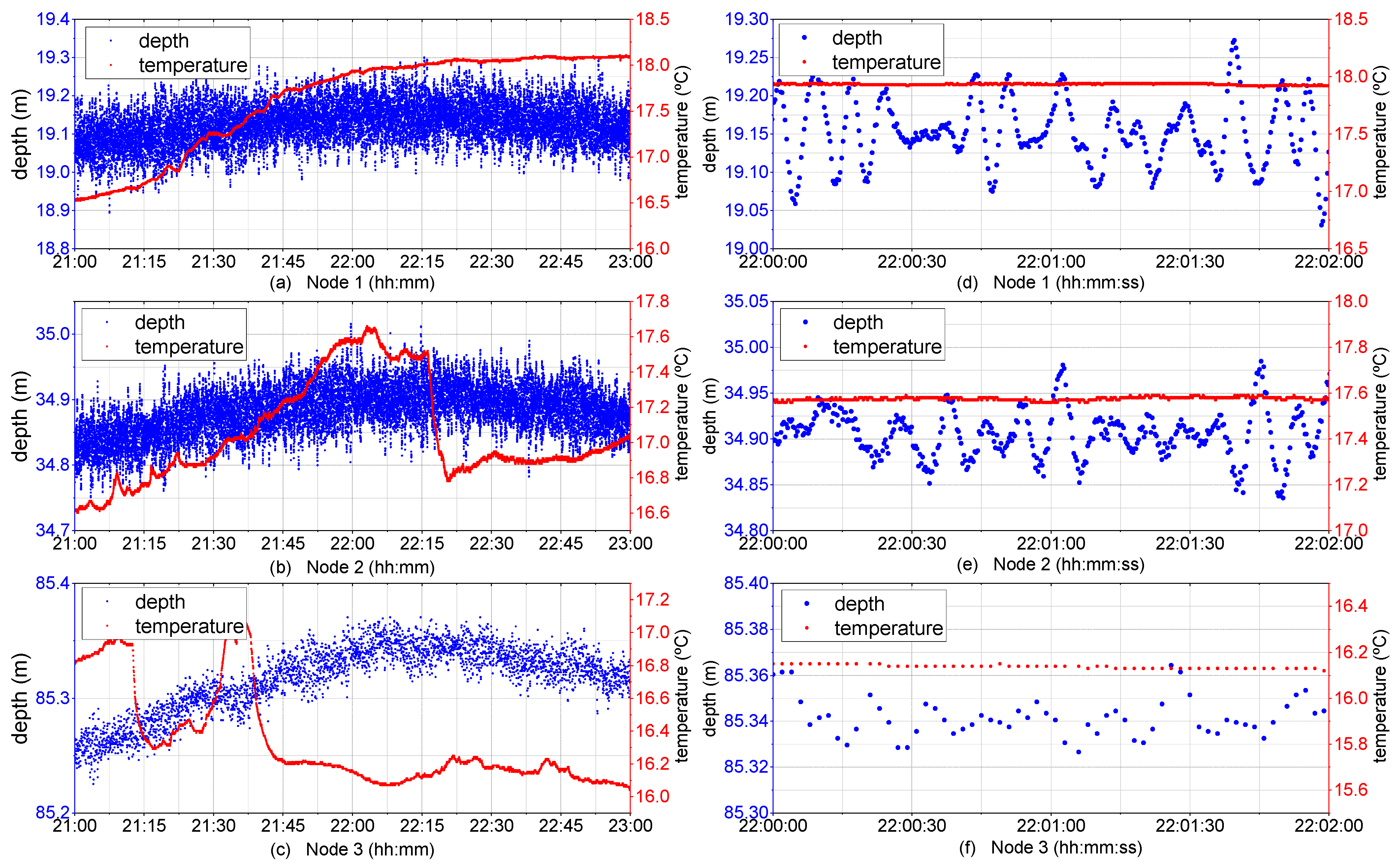
Figure 2 presents the water temperature (red circles) and depth measurements (blue circles) gathered from all three sensor stations between 21:00 and 23:00 on 8 September 2023. The temperature was directly measured by the MS5837-30BA sensor, while the depth was derived from its pressure measurements using Equation (1).
The collected data reveal that the repeater nodes 1, 2 and 3 were deployed at seafloor depths of approximately 19, 34 and 85 m, respectively. The depth signals from all three stations exhibit a slow variation in the average depth due to tidal effects. The observation window coincides with a high tide period, peaking around 22:15, which is reflected in
Figure 2a–c. Additionally, these graphs display high-frequency variations in the depth signals, corresponding to pressure fluctuations caused by wave activity.
Figure 2d–f provide a detailed insight into these variations over a 2 min interval, illustrating the propagation of sea waves. It is important to note that the wave characteristics observed are quite similar, as the repeater nodes are in the same coastal area. However, the recorded depth variations (wave amplitudes) differ: node 1 shows the largest wave amplitude (
Figure 2d), while node 3 shows the smallest (
Figure 2f). This is consistent with the expected pressure attenuation with depth, as Equation (13) describes. Another key observation is that while nodes 1 and 2 recorded data with a sampling period of 0.3 s, node 3 recorded data with 1 s. Although wave propagation is still detectable in
Figure 2f, the data are less detailed compared to
Figure 2d,e.
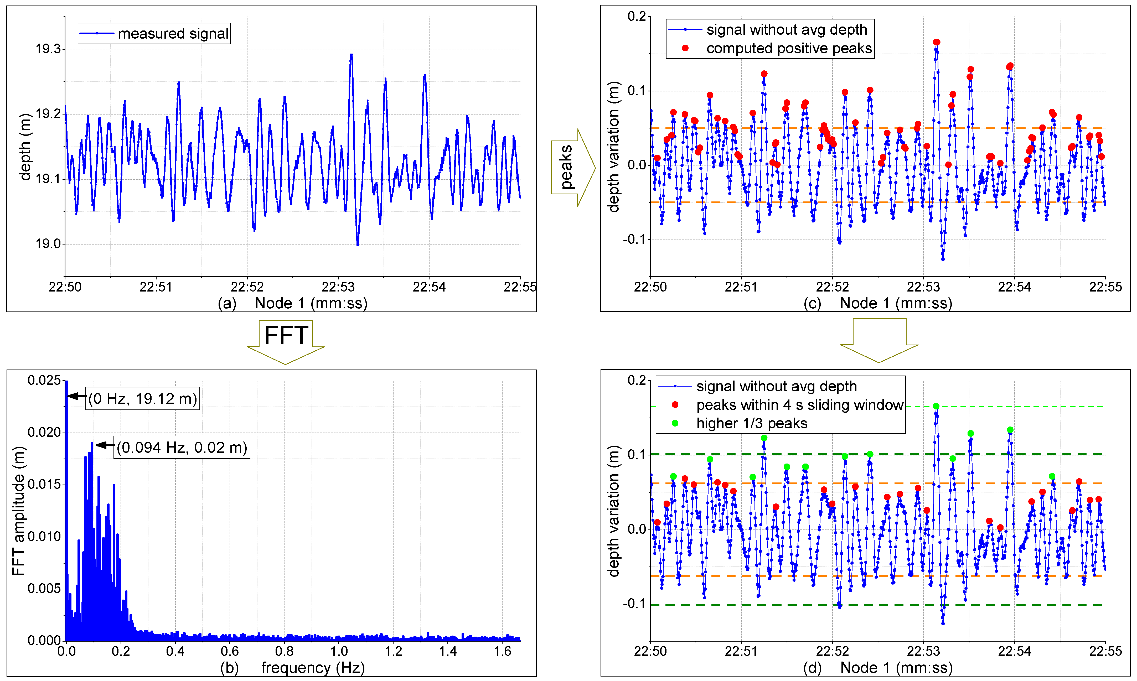
Figure 3 illustrates the step-by-step processing methods used to estimate the wave period and significant wave height from the measured depth data. The analysis spans a 5 min window, from 22:50 to 22:55, of the collected measurements from the sensor station of node 1 depicted in
Figure 2a.
In
Figure 3b, the signal is processed using an FFT to convert the time-domain signal into its frequency components, applying Equations (2) and (4). From the frequency analysis, the FFT amplitude at 0 Hz is retrieved, corresponding to the water column height (depth), along with the next most substantial frequency component (0.094 Hz or 10.64 s if using Equation (3)). However, while this is the most significant frequency, the spectrum between 0.07 and 0.18 Hz (5.5–14.3 s) also shows relevant energy. This, combined with the non-stationary nature of the depth variation signal, causes the calculated amplitude of the targeted frequency (0.094 Hz, 0.02 m) to be lower than the observed wave amplitude magnitudes seen in the depth signal of
Figure 3a.
Given that the FFT is not a precise method for estimating wave amplitude, this task is accomplished by employing the developed peaks algorithm.
Figure 3c shows the depth variation after removing the average depth of the original signal using Equations (5) and (6), and it also displays the computed positive peaks using Equation (7). For demonstration purposes, the dashed orange line illustrates the average amplitude of the detected positive peaks (0.05 m), which already offers a better estimation than the calculated FFT amplitude. In this time set, the signal appears clean; however, others may contain noise. Therefore, the 4 s sliding window is applied to remove erroneous peaks, using Equation (8), in order to only retain those corresponding to wave crests (
Figure 3d). By applying Equation (9), the highest one-third of the peaks are identified, and the significant wave amplitude (dashed dark-green line) is calculated using Equation (10).
Figure 3d highlights the difference between the values of the average wave peaks (dashed orange line, 0.062 m) and the average of the top one-third of the peaks (dashed dark-green line, 1.102 m). Additionally, using Equation (11), the algorithm can also compute the highest peaks within the time set (dashed light-green line, 0.166 m).
After validating the wave period using the FFT and determining the significant wave amplitude through the peaks algorithm, the next step involved calculating the experimental coefficient to convert the depth variations measured by the sensors into surface wave amplitude using Equation (13). The two-hour dataset presented in
Figure 2a–c was used for this calibration. The IPMA forecast for the wave period during this time window was 11 s, closely aligning with the values calculated using the FFT.
Table 1 summarises the calculated wave period, sensor depth and wave amplitude, alongside the wave period and wave height obtained from the IPMA forecast (note that wave amplitude is half of the wave height). The experimental coefficient was derived from these values. This process calibrated the sensors to accurately monitor significant wave heights, which was used in the subsequent data analysis.
After calibration, the sensor stations were activated for 58 h of continuous monitoring, from 22:00 on 12 September to 08:00 on 15 September 2023. During this period, the stations collected pressure data, which were analysed using both the FFT and peaks algorithm methods to provide hourly wave period and significant wave height estimations. Data collection was interrupted three times: from 06:00 to 07:00 on 12 September due to a power outage on land and from 08:00 to 09:00 and 10:00 to 11:00 on 13 September for maintenance. Additionally, a watertightness malfunction in the sensor of node 1 was detected, causing the respective sensor station to stop transmitting data.
Figure 4 presents the depth measurements and estimations for the average wave period and significant wave height for nodes 2 and 3 during the 58 h monitoring period.
Given the extended monitoring window,
Figure 4a,b now reveal the complete tidal cycle, showing a depth variation of approximately 2 m from low to high tides, as detected by both nodes. The depth data were processed as previously described, enabling the estimation of the dominant wave period using the FFT method and the significant wave height via the peaks algorithm. To assist in result interpretation, high tide peaks are marked with dashed black-green lines and low tide peaks with dashed light-blue lines.
Between 12 September and the night of 14 September, IPMA’s forecast wave periods ranged from 9 to 11 s, with a sudden increase to 15 s in the early hours of 15 September. Both node 2 and node 3 successfully detected this shift.
Figure 4c shows a comparison between the sensor stations’ estimations and the IPMA forecast. Although the estimated wave periods are slightly higher than the forecast, the results of node 2 show an average difference of only 1.5 s, a reasonable margin given the 1 s resolution of the IPMA forecast. On the other hand, the estimation of node 3 exhibits higher variability and error, likely attributable to the longer 1 s sampling interval used.
Regarding significant wave height, the IPMA forecast indicated a stable range between 0.8 and 0.9 m, with a slight increase to 1.1 m on the evening of 13 September. The estimations from the sensor stations do not closely align with this trend and exhibit considerable differences. It is important to note that IPMA forecasts are based on numerical models applied to extensive maritime regions. While wave periods are generally expected to remain consistent within a localised area, the same cannot be said for wave heights. This discrepancy arises because forecasts are primarily made for open sea conditions, where wave heights are typically smaller. Nevertheless, they tend to increase as waves approach the coast—where the marine cable was installed. Therefore, both results and forecasts regarding wave height should be interpreted cautiously.
Figure 4d illustrates that the average values of the estimations from both nodes align with the forecast. However, their raw values exhibit variations not observed in the forecast. A detailed analysis of the estimations reveals a consistent pattern between both nodes, where wave height significantly increases during flood tide and decreases just before reaching high tide. This phenomenon is commonly observed in coastal regions, where wave heights tend to be higher during flood and/or high tides and lower during ebb and/or low tides. Accordingly, the results suggest that during the monitored period, both nodes recorded an increase in wave height attributed to tidal waves, in contrast to wind waves. Regarding the estimations for the wave period, node 3 shows a more significant variance than node 2, which can be attributed to the differing sampling periods and the increased depth, making it more challenging to capture wave propagation effectively.
4. Discussion
The results presented in this study highlight several key insights regarding the capabilities and performance of the deployed sensor stations for wave monitoring in coastal areas using marine cable infrastructure. We validated the monitoring system’s effectiveness through the combination of pressure data analysis, the FFT for wave period estimation and the peaks algorithm for significant wave height estimation.
The data collected in this study relied on the MS5837-30BA sensor. Despite being deployed at different depths (19 m, 34 m and 85 m for nodes 1, 2 and 3, respectively), the sensor stations consistently recorded tidal fluctuations with an amplitude of approximately 2 m, aligning well with expected tidal cycles. Despite the varying depths, the coherence of the pressure data across all three nodes demonstrates the accuracy and reliability of the MS5837-30BA sensor in capturing both short-term wave fluctuations and longer tidal cycles. Additionally, the fact that this is a low-cost sensor further underscores its advantage for extended monitoring applications in marine environments. Its affordability combined with its precision makes it a viable solution for large-scale deployments, particularly in projects with limited budgets or those requiring multiple sensing locations.
Beyond tidal monitoring, the pressure data also enabled the estimation of sea wave characteristics, particularly the wave period and wave height. While the wave period estimates closely aligned with the IPMA forecasts—showing an average difference of 1.5 s for node 2—the wave height estimations displayed more significant variation. However, the coherence in the variations detected by nodes 2 and 3, as well as the patterns observed concerning tidal cycles, provides confidence in the measurements. The link between tidal cycles and wave height was obvious, with both nodes consistently recording higher wave heights during flood tides. This phenomenon is well documented in coastal hydrodynamics, where tidal currents can amplify or dampen wave energy, but it is not reflected in the IPMA forecasts. This discrepancy is likely due to the difference between the numerical models used for open-water forecasts and the localised conditions at the sensor station sites, which are closer to the shore. These findings highlight the importance of considering spatial variability in wave height caused by factors such as wave shoaling, reflection and diffraction as waves approach shallow waters—conditions that numerical models may not fully capture. As a result, the experimental coefficients derived during the calibration process using IPMA’s wave height forecasts may also not be entirely accurate. Future calibration and validation efforts should take this into account and explore alternative ground-truth sources, such as local surface buoys or ADCPs, to provide more precise wave height estimations.
Another important outcome of this work is the relationship between depth, sampling period and the performance of the wave estimation process. As anticipated, the sensor at node 3, positioned at a depth of 85 m, encountered greater difficulty in detecting wave propagation compared to the shallower nodes 1 and 2. This highlights the attenuation of pressure signals with depth, which makes accurate wave height estimations increasingly challenging at deeper locations. Moreover, the difference in sampling periods—0.3 s for node 2 and 1 s for node 3—also contributed to the discrepancies observed in wave period and amplitude estimations. The lower sampling frequency at node 3 likely resulted in higher variance in the recorded data, particularly in wave period estimations. These findings emphasise the importance of higher sampling frequencies at deeper installations to better capture wave propagation dynamics and improve estimation accuracy.
Even though the primary focus of this work was not water temperature, the sensor stations, equipped with the MS5837-30BA sensor, successfully captured temperature data throughout the monitoring period.
Figure 2 highlights a temperature gradient from node 1 to node 3, demonstrating a decrease in temperature with increasing depth, which is characteristic of thermal stratification in marine environments—warmer temperatures near the surface and cooler conditions at the seafloor. Additionally,
Figure 4 reveals local fluctuations in water temperature during the ebb and flood tides, with node 2 showing an increase in temperature during both cycles, while node 3 experienced a rise in temperature predominantly during flood tides. These patterns suggest the potential influence of ocean currents during tidal cycles in the region, which could be mapped in greater detail by increasing the spatial resolution with additional sensor nodes. Although water temperature data were not directly relevant to the wave characteristic estimations, they demonstrate the versatility and potential of smart marine cables for comprehensive ocean monitoring.
The integration of sensors into marine cable infrastructure opens new opportunities for tracking a variety of oceanographic parameters. Advanced computational processing, including artificial intelligence and machine learning, can enhance data interpretation by identifying patterns, detecting anomalies and improving predictive modelling. These technologies enable the real-time processing of vast datasets, allowing for the extraction of valuable insights into ocean dynamics. By leveraging AI-driven analytics, marine cables can evolve into intelligent monitoring networks, autonomously adapting to environmental changes and expanding their role in global ocean observation systems. With the vast network of submarine cables already in place, providing reliable power supply and broadband capacity for real-time data transmission via optical fibre, smart marine cables represent a promising frontier for next-generation ocean monitoring systems. This infrastructure can be leveraged to develop a more extensive and detailed understanding of ocean dynamics, including parameters such as temperature, pressure, salinity and wave activity, transforming marine cables into multi-purpose monitoring platforms that can contribute significantly to both scientific research and environmental management.
5. Conclusions
This study investigates the potential of integrating sensor technology into marine cable infrastructure for real-time oceanographic monitoring, demonstrating successful measurements of tidal cycles and wave characteristics using the MS5837-30BA pressure sensor. A 2000 m marine cable demonstrator, deployed off the coast of Sesimbra, Portugal, was equipped with three active repeater nodes. These nodes supported various subsystems, including AUV operations, soundscape processing and oceanographic monitoring. Each repeater node, installed at different depths, was outfitted with sensor stations that effectively captured the expected tidal depth variations. Data collected from these stations were consistent and coherent across the nodes, validating the utility of these low-cost sensors in marine monitoring applications, where scalability and affordability are essential.
The primary focus of this work was on monitoring sea wave characteristics. The hourly wave period was estimated through FFT analysis of the collected pressure data. A custom algorithm was developed to detect wave crests and estimate both significant and maximum wave height. The results were promising, with wave period estimates closely aligning with forecasts. The observed correlation between tidal cycles and wave height—particularly the increase in wave heights during flood tides—demonstrated the system’s sensitivity to coastal hydrodynamics. While wave height estimates showed greater deviations from forecasts, this was likely due to the spatial variability of wave heights as waves approach the coast, a factor that numerical models designed for open waters often fail to capture. This underscores the importance of localised monitoring to complement and refine large-scale models, especially in coastal regions. Additionally, the study underscored the challenges associated with deep-water sensor installations, where both pressure signal attenuation and lower sampling rates introduced higher variances in the data. Complementary use of an experimental coefficient was introduced using forecast data to calibrate the sensor stations. This highlights the need for optimised sensor configurations, including higher sampling frequencies, to ensure accurate wave characteristic estimations in deeper waters.
Tidal and sea condition monitoring is critical for both coastal and open-sea applications. Along the coast, accurate tidal data can inform beach management, coastal erosion prevention and marine traffic control, ensuring safer navigation and port operations. In open waters, real-time tidal monitoring can potentially improve tsunami detection and early warning systems. This dual utility underscores the value of sensor-integrated marine cables for a broad range of maritime operations, from safety to environmental protection. Overall, this study demonstrates the wider potential of integrating monitoring stations into submarine cable infrastructure. With their extensive reach, power availability and data transmission capacity, smart marine cables offer a transformative opportunity for future oceanographic monitoring. These systems could extend beyond wave and tide measurements to monitor a wide range of environmental parameters, providing a more comprehensive and high-resolution understanding of ocean dynamics. The successful application of sensors in marine cables in this study paves the way for scalable, real-time ocean monitoring solutions that can support both scientific research and environmental management, contributing to more informed decision making for the sustainable use of marine resources.
Author Contributions
Conceptualisation, T.M. and J.L.R.; methodology, T.M. and J.L.R.; software, T.M.; validation, all authors; formal analysis, T.M.; investigation, T.M.; resources, M.S.M.; data curation, T.M.; writing—original draft preparation, T.M.; writing—review and editing, all authors; visualisation, all authors; supervision, M.S.M. and L.M.G.; project administration, M.S.M.; funding acquisition, M.S.M. All authors have read and agreed to the published version of the manuscript.
Funding
This work was funded by the project K2D: Knowledge and Data from the Deep to Space under reference POCI-01-0247-FEDER-045941, co-financed by the European Regional Development Fund (ERDF) through the Operational Programme for Competitiveness and Internationalisation (COMPETE2020) and by the Portuguese Foundation for Science and Technology (FCT) under the MIT Portugal Program.
Data Availability Statement
The original contributions presented in the study are included in the article. Further inquiries can be directed to the corresponding author.
Acknowledgments
The authors wish to express their gratitude to the commander and crew of the NRP Andromeda from the Portuguese Navy for their support during the installation of the marine cable demonstrator.
Conflicts of Interest
The authors declare no conflicts of interest.
Abbreviations
The following abbreviations are used in this manuscript:
| AUV | Autonomous Underwater Vehicle |
| ECMWF | European Centre for Medium-Range Weather Forecasts |
| FFT | Fast Fourier Transform |
| GPS | Global Positioning System |
| HF | High Frequency |
| HRES-WAM | High RESolution WAve Model |
| IPMA | Instituto Português do Mar e da Atmosfera |
| K2D | Knowledge and Data from the Deep to Space |
| LIDAR | Light Detection and Ranging |
| NRP | Navio da Republica Portuguesa |
| PCB | Printed Circuit Board |
| PoE | Power over Ethernet |
| UART | Universal Asynchronous Receiver/Transmitter |
| VDC | Volts Direct Current |
References
- Li, Z.; Tang, T.; Li, Y.; Draycott, S.; van den Bremer, T.S.; Adcock, T.A.A. Wave loads on ocean infrastructure increase as a result of waves passing over abrupt depth transitions. J. Ocean Eng. Mar. Energy 2023, 9, 309–317. [Google Scholar] [CrossRef]
- Xu, J.; Gong, J.; Li, Y.; Fu, Z.; Wang, L. Surf-riding and broaching prediction of ship sailing in regular waves by LSTM based on the data of ship motion and encounter wave. Ocean Eng. 2024, 297, 117010. [Google Scholar] [CrossRef]
- van Wiechen, P.P.J.; de Vries, S.; Reniers, A.J.H.M. Field observations of wave-averaged suspended sediment concentrations in the inner surf zone with varying storm conditions. Mar. Geol. 2024, 473, 107302. [Google Scholar] [CrossRef]
- Baleani, C.A.; Menéndez, M.C.; Vitale, A.J.; Amodeo, M.R.; Perillo, G.M.E.; Piccolo, M.C. Assessing the role of tidal cycle, waves, and wind as drivers of surf zone zooplankton on a temperate sandy beach. Reg. Stud. Mar. Sci. 2024, 73, 103455. [Google Scholar] [CrossRef]
- Thompson, M.E.; Atkinson, A.; Watterson, E.; Naderi, N.; Loehr, H.; Baldock, T.E. A camera based method for assessing surf amenity of submerged nearshore structures in a wave basin by quantifying wave breaking. Ocean Eng. 2023, 286, 115606. [Google Scholar] [CrossRef]
- Aravind, P.; Amrutha, M.M.; Kumar, V.S. Ocean wave dynamics in the coastal area of the central west coast of India and its variability. Ocean Eng. 2021, 227, 108880. [Google Scholar] [CrossRef]
- Ahn, S. Modeling mean relation between peak period and energy period of ocean surface wave systems. Ocean Eng. 2021, 228, 108937. [Google Scholar] [CrossRef]
- Curto, D.; Franzitta, V.; Guercio, A. Sea Wave Energy. A Review of the Current Technologies and Perspectives. Energies 2021, 14, 6604. [Google Scholar] [CrossRef]
- Caloiero, T.; Aristodemo, F.; Ferraro, D.A. Annual and seasonal trend detection of significant wave height, energy period and wave power in the Mediterranean Sea. Ocean Eng. 2022, 243, 110322. [Google Scholar] [CrossRef]
- Sadeghifar, T.; Lama, G.F.C.; Sihag, P.; Bayram, A.; Kisi, O. Wave height predictions in complex sea flows through soft-computing models: Case study of Persian Gulf. Ocean Eng. 2022, 245, 110467. [Google Scholar] [CrossRef]
- Marimon, M.C.; Tangonan, G.; Libatique, N.J.; Sugimoto, K. Development and evaluation of wave sensor nodes for ocean wave monitoring. IEEE Syst. J. 2015, 9, 292–302. [Google Scholar] [CrossRef]
- Bender, I.C.; Guinasso, J.L.; Walpert, J.N.; Howden, S.D. A Comparison of Methods for Determining Significant Wave Heights—Applied to a 3-m Discus Buoy during Hurricane Katrina. J. Atmos. Ocean. Technol. 2010, 27, 1012–1028. [Google Scholar] [CrossRef]
- Babanin, A.V.; Verkeev, P.P.; Krivinsky, B.B.; Proshchenko, V.G. Measurement of wind waves by means of a buoy accelerometer wave gauge. Phys. Oceanogr. 1993, 4, 399–407. [Google Scholar] [CrossRef]
- Pedersen, T.; Siegel, E.; Wood, J. Directional wave measurements from a subsurface buoy with an acoustic wave and current profiler (AWAC). In Proceedings of the OCEANS 2007, Vancouver, BC, Canada, 29 September–4 October 2007. [Google Scholar] [CrossRef]
- Zhou, B.; Zhang, X.; Wan, X.; Liu, T.; Liu, Y.; Huang, H.; Chen, J. Development and Application of a Novel Tsunami Monitoring System Based on Submerged Mooring. Sensors 2024, 24, 6048. [Google Scholar] [CrossRef]
- D’Asaro, E. Surface Wave Measurements from Subsurface Floats. J. Atmos. Ocean. Technol. 2015, 32, 816–827. [Google Scholar] [CrossRef]
- Ponce de León, P.; Bettencourt, J.H.; Ringwood, J.V.; Benveniste, J. Assessment of combined wind and wave energy in European coastal waters using satellite altimetry. Appl. Ocean Res. 2024, 152, 104184. [Google Scholar] [CrossRef]
- Stopa, J.E. Seasonality of wind speeds and wave heights from 30 years of satellite altimetry. Adv. Space Res. 2021, 68, 787–801. [Google Scholar] [CrossRef]
- Ponce de León, S.; Bettencourt, J.H. Composite analysis of North Atlantic extra-tropical cyclone waves from satellite altimetry observations. Adv. Space Res. 2021, 68, 762–772. [Google Scholar] [CrossRef]
- Benetazzo, A.; Barbariol, F.; Bergamasco, F.; Torsello, A.; Carniel, S.; Sclavo, M. Stereo wave imaging from moving vessels: Practical use and applications. Coast. Eng. 2016, 109, 114–127. [Google Scholar] [CrossRef]
- Sallam, O.; Feng, R.; Stason, J.; Wang, X.; Fürth, M. Stereo vision based systems for sea-state measurement and floating structures monitoring. Signal Process. Image Commun. 2024, 122, 117088. [Google Scholar] [CrossRef]
- Nouguier, F.; Grilli, S.T.; Guérin, C.A. Nonlinear ocean wave reconstruction algorithms based on simulated spatiotemporal data acquired by a flash LIDAR camera. IEEE Trans. Geosci. Remote Sens. 2014, 52, 1761–1771. [Google Scholar] [CrossRef]
- Dankert, H.; Rosenthal, W. Ocean surface determination from X-band radar-image sequences. J. Geophys. Res. Ocean. 2004, 109, 4016. [Google Scholar] [CrossRef]
- Johnson, J.T.; Burkholder, R.J.; Toporkov, J.V.; Lyzenga, D.R.; Plant, W.J. A numerical study of the retrieval of sea surface height profiles from low grazing angle radar data. IEEE Trans. Geosci. Remote Sens. 2009, 47, 1641–1650. [Google Scholar] [CrossRef]
- Ardhuin, F.; Balanche, A.; Stutzmann, E.; Obrebski, M. From seismic noise to ocean wave parameters: General methods and validation. J. Geophys. Res. Ocean. 2012, 117, 5002. [Google Scholar] [CrossRef]
- Ferretti, G.; Barani, S.; Scafidi, D.; Capello, M.; Cutroneo, L.; Vagge, G.; Besio, G. Near real-time monitoring of significant sea wave height through microseism recordings: An application in the Ligurian Sea (Italy). Ocean Coast. Manag. 2018, 165, 185–194. [Google Scholar] [CrossRef]
- Höttges, A.; Smaadahl, M.; Evers, F.M.; Boes, R.M.; Rabaiotti, C. Dynamic Wave Measurement with a High Spatial Resolution Distributed Fiber Optic Pressure Sensor. IEEE Sens. J. 2024, 24, 22387–22396. [Google Scholar] [CrossRef]
- Arkwright, J.W.; Underhill, I.D.; Maunder, S.A.; Jafari, A.; Cartwright, N.; Lemckert, C. Fiber optic pressure sensing arrays for monitoring horizontal and vertical pressures generated by traveling water waves. IEEE Sens. J. 2014, 14, 2739–2742. [Google Scholar] [CrossRef]
- Pereira, E.; Tieppo, M.; Faria, J.; Hart, D.; Lermusiaux, P. Subsea Cables as Enablers of a Next Generation Global Ocean Sensing System. Oceanography 2023, 36, 70–71. [Google Scholar] [CrossRef]
- Howe, B.M.; Arbic, B.K.; Aucan, J.; Barnes, C.R.; Bayliff, N.; Becker, N.; Butler, R.; Doyle, L.; Elipot, S.; Johnson, G.C.; et al. Smart cables for observing the global ocean: Science and implementation. Front. Mar. Sci. 2019, 6, 434290. [Google Scholar] [CrossRef]
- Chen, C.F.; Chan, H.-C.; Chang, R.-I.; Tang, T.-Y.; Jan, S.; Wang, C.-C.; Wei, R.-C.; Yang, Y.-J.; Chou, L.-S.; Shin, T.-C.; et al. Data demonstrations on physical oceanography and underwater acoustics from the MArine Cable Hosted Observatory (MACHO). In Proceedings of the 2012 Oceans-Yeosu, Yeosu, Republic of Korea, 21–24 May 2012. [Google Scholar] [CrossRef]
- Cruz, N.A.; Silva, A.; Zabel, F.; Ferreira, B.; Jesus, S.M.; Martins, M.S.; Pereira, E.; Matos, T.; Viegas, R.; Rocha, J.; et al. A Demonstrator for Future Fiber-Optic Active SMART Repeaters. In Proceedings of the OCEANS 2024-Singapore, Singapore, 15–18 April 2024. [Google Scholar] [CrossRef]
- Duarte, R.; Zabel, F.; Silva, A.; Jesus, S.M. Soundscaping Using a Smart Cable Prototype Off the Coast of Portugal. In Proceedings of the OCEANS 2024-Singapore, Singapore, 15–18 April 2024. [Google Scholar] [CrossRef]
- Baptista, J.P.; Matos, T.; Lopes, S.F.; Faria, C.L.; Magalhaes, V.H.; Vieira, E.M.F.; Martins, M.S.; Goncalves, L.M.; Brito, F. A four-probe salinity sensor optimized for long-term autonomous marine deployments. In Proceedings of the OCEANS 2019-Marseille, Marseille, France, 17–20 June 2019. [Google Scholar] [CrossRef]
- Monteiro, M.J.; Couto, F.T.; Bernardino, M.; Cardoso, R.M.; Carvalho, D.; Martins, J.P.A.; Santos, J.A.; Argain, J.L.; Salgado, R. A Review on the Current Status of Numerical Weather Prediction in Portugal 2021: Surface–Atmosphere Interactions. Atmosphere 2022, 13, 1356. [Google Scholar] [CrossRef]
- Janssen, P.; Bidlot, J.-R.; Abdalla, S.; Hersbach, H. Progress in Ocean Wave Forecasting at ECMWF, ECMWF Tech. Memo. 2005, 27. Available online: https://www.ecmwf.int/sites/default/files/elibrary/2005/10187-progress-ocean-wave-forecasting-ecmwf.pdf (accessed on 25 March 2025).
- Bidlot, J.-R. Present status of wave forecasting at ECMWF. In Proceedings of the Workshop on Ocean Waves, Reading, UK, 25–27 June 2012; Available online: https://www.ecmwf.int/en/elibrary/73712-present-status-wave-forecasting-ecmwf (accessed on 25 March 2025).
- Reikard, G.; Pinson, P.; Bidlot, J.R. Forecasting ocean wave energy: The ECMWF wave model and time series methods. Ocean Eng. 2011, 38, 1089–1099. [Google Scholar] [CrossRef]
- Brousseau, P.; Seity, Y.; Ricard, D.; Léger, J. Improvement of the forecast of convective activity from the AROME-France system. Q. J. R. Meteorol. Soc. 2016, 142, 2231–2243. [Google Scholar] [CrossRef]
- Seity, Y.; Brousseau, P.; Malardel, S.; Hello, G.; Bénard, P.; Bouttier, F.; Lac, C.; Masson, V. The AROME-France Convective-Scale Operational Model. Mon. Weather Rev. 2011, 139, 976–991. [Google Scholar] [CrossRef]
| Disclaimer/Publisher’s Note: The statements, opinions and data contained in all publications are solely those of the individual author(s) and contributor(s) and not of MDPI and/or the editor(s). MDPI and/or the editor(s) disclaim responsibility for any injury to people or property resulting from any ideas, methods, instructions or products referred to in the content. |
© 2025 by the authors. Licensee MDPI, Basel, Switzerland. This article is an open access article distributed under the terms and conditions of the Creative Commons Attribution (CC BY) license (https://creativecommons.org/licenses/by/4.0/).


