High-Precision Surfacing Position Prediction for Underwater Gliders via Coordinate Transformation

Abstract

The accurate prediction of the surfacing position of underwater gliders (UGs) is critical for mission success and cost-effective retrieval. However, current state-of-the-art (SOTA) methods often rely on complex multi-model integrations or large volumes of ocean current data, thereby increasing operational costs and system complexity. In this study, we systematically introduce—for the first time—a coordinate-transformation-based prediction framework, originally applied in other navigation contexts, into the UG surfacing-position-prediction task. By projecting both the glider’s entry and surfacing positions into a Universal Transverse Mercator (UTM) planar coordinate system and treating the resulting displacement as the prediction target, we avoid dependence on heavily parameterized current models, simplify the training process, and maintain robust predictive accuracy. Our approach combines common machine learning predictors (e.g., AdaBoost, LGBM, gradient boosting, random forest, decision trees) instead of advanced deep learning architectures, thus reducing computational overhead. Experiments on two real-world sea trial datasets (containing 2159 and 1456 profiles, respectively) show that, compared with direct regression approaches, this method improves positioning accuracy by up to 50% within a 500-meter range, yet requires minimal multi-source data. Overall, this study integrates the concept of coordinate transformation into the task of predicting the surfacing position of underwater gliders, effectively streamlining the method without sacrificing accuracy. The result is a highly flexible and cost-effective approach, providing theoretical support for future optimizations of underwater glider navigation systems.

1. Introduction

Autonomous underwater vehicles (AUVs) are robot devices with autonomous navigation and are widely used in fields such as ocean exploration, environmental monitoring, and underwater surveying. AUVs can perform complex tasks, such as seabed mapping and environmental data collection, without human intervention [1,2,3,4,5]. Due to their high maneuverability and adaptability, AUVs are increasingly valued for application in deep-sea and extreme environments.

In the design and control of AUVs, precise modeling is crucial. Traditional modeling methods often rely on physical models and empirical formulas [6,7,8]; however, these methods may have limitations when dealing with complex fluid dynamics and environmental changes. Therefore, in recent years, machine learning (ML) techniques have been introduced into AUV modeling and control to enhance their performance and adaptability [9,10,11].

The authors of [12] indicate that artificial neural networks (ANNs) are used to model adaptive trajectory tracking control schemes to address the issues of unknown asymmetric actuator saturation and various unknown dynamics. Specifically, researchers utilize neural networks to relate the hydrodynamics of complex AUVs to the derivatives of the desired tracking speeds, thereby improving the stability and responsiveness of the control system. Additionally, the author of [13] mentions the adoption of a bilateral adaptive control scheme that incorporates radial basis function neural networks to achieve force and position coordination in the remote operating system of underwater vehicles. This approach effectively responds to external disturbances and uncertainties, enabling precise position tracking. These applications demonstrate that machine learning can significantly enhance the control accuracy of AUVs and their adaptability in complex environments.

An underwater glider is a specific type of AUV that primarily glides through the water by changing its buoyancy and attitude, utilizing the buoyancy and gravity in the water for efficient underwater movement. Underwater gliders are typically used for long-duration ocean monitoring and data collection, offering high endurance. The unique buoyancy-driven mechanism of underwater gliders provides them with significant advantages in deep-sea exploration and environmental monitoring [14,15,16,17]. However, this buoyancy-driven mechanism inherently restricts the glider’s speed, rendering it particularly susceptible to fluctuations in ocean currents. Such sensitivity can result in significant deviations from the intended trajectory, influenced by various environmental factors. Furthermore, the relatively simplistic dynamic structure of gliders, while beneficial in terms of reducing maintenance requirements, concurrently diminishes their control capabilities in intricate marine environments, thereby complicating the task of adhering to the desired path. Consequently, the accurate prediction of the glider’s surfacing position becomes critically important. Enhanced precision in surfacing position predictions not only increases the likelihood of successful glider missions but also mitigates the expenditure of time and resources in ocean observation endeavors. This is essential for the effective operation of gliders within complex marine settings.

By contrast, large errors in surfacing position prediction can have serious practical consequences. For instance, if a glider surfaces far from its expected location, search-and-recovery teams may fail to promptly locate it, potentially leading to mission failure. In such cases, the glider and the valuable data it carries would be lost. Even when recovery is possible, substantial prediction errors can greatly increase mission costs: vessels may have to search wide areas, thus consuming extra time and fuel and causing the overall operational efficiency to suffer. In extreme scenarios, a missed glider recovery due to inaccurate surfacing estimates could turn a routine retrieval into an urgent, costly search mission.

However, current state-of-the-art surfacing prediction methods face significant technical hurdles in real-world deployments. Many approaches based on detailed dynamic modeling or multi-model data fusion require large volumes of high-quality oceanographic data (e.g., current profiles) and carefully tuned parameters. This heavy data dependence can be problematic, since obtaining and updating such data in real time is often impractical. Deep learning models have shown promise, but complex network structures demand considerable computational resources and may not run fast enough for real-time use on resource-limited platforms. Some hybrid strategies combine physics-based models with machine learning or multiple learning models together to improve accuracy, but these systems tend to be intricate and difficult to maintain. Moreover, training or predicting directly in geographic latitude–longitude coordinates introduces nonlinear distortion issues, as the Earth’s curved surface does not translate linearly to distance; this geodetic nonlinearity can degrade prediction accuracy if not properly handled. In summary, existing mainstream methods often struggle with high data requirements, high model complexity, poor real-time performance, and geographic coordinate nonlinearity, which collectively hinder their utility in operational glider missions.

In light of these challenges, this study aims to develop a more practical and robust surfacing position prediction approach that achieves high precision while minimizing deployment complexity and cost. We are particularly motivated to address the nonlinearities of geodetic coordinates and the over-reliance on complex models. To this end, our method introduces a coordinate transformation technique coupled with a lightweight predictive model. By projecting the glider’s entry and surfacing locations into a planar coordinate system (e.g., the Universal Transverse Mercator, UTM) and predicting the surfacing displacement in that coordinate frame, we transform the problem into a more linear one. This strategy avoids the need for heavily parameterized ocean current models and simplifies the learning task, since the planar displacement is easier for a model to learn than raw latitude–longitude differences. The use of a single, lightweight ML model (instead of an ensemble of multiple models) further reduces computational load and algorithmic complexity, ensuring the solution can run in real time on limited hardware. In essence, our approach seeks to improve prediction accuracy through coordinate frame simplification while lowering the implementation and maintenance costs associated with deployment.

Building on previous work and cross-domain insights, this study proposes a displacement prediction framework for underwater gliders based on coordinate transformation. The proposed approach substantially streamlines the prediction pipeline without sacrificing accuracy: a one-time conversion of coordinates provides a cleaner, linear displacement feature for model training, and a single-model prediction yields results comparable to more complex multi-model methods. We validate the effectiveness of this approach using two sets of real sea trial data from different ocean regions, demonstrating that the coordinate transformation method can significantly improve surfacing position accuracy and stability across various scenarios. The results show that our method can achieve higher precision with lower complexity, which in turn reduces mission costs and improves the reliability of glider retrieval.

The structure of the paper is as follows: Section 2 reviews the current research status and challenges related to the positioning or trajectory prediction of underwater gliders, elucidating the shortcomings of existing methods and research gaps. Section 3 introduces the dataset and the coordinate transformation-displacement prediction method used in the experiments, including model principles and hyperparameter selection. Section 4 presents comparative experimental results of several machine learning algorithms on the real sea trial dataset, discussing error distribution and stability. Section 5 further analyzes the applicability of the method concerning issues such as the span of marine areas and ocean current modeling based on the experimental results. Section 6 summarizes the main contributions and shortcomings of this research and discusses future work directions.

2. Related Work

In this section, we review and analyze existing studies related to trajectory prediction for underwater gliders, both domestically and internationally, highlighting the strengths and limitations of current methods and clearly defining the critical issues addressed by this research. To facilitate reader comprehension, this chapter is specifically structured into the following subsections:

Section 2.1 summarizes representative studies from other domains where coordinate transformations have been successfully utilized for trajectory prediction tasks, highlighting the potential advantages and insights of coordinate transformations for addressing geographical nonlinearities.

Section 2.2 provides a detailed analysis of existing trajectory prediction approaches specifically applied to underwater gliders, emphasizing their limitations in terms of data dependence, model complexity, and real-time operational constraints.

Section 2.3, based on the analyses presented in the preceding two subsections, further explores the motivation and potential benefits of integrating coordinate transformation methods into underwater glider trajectory prediction, clearly identifying the innovative starting point and rationale of the present study.

Section 2.4 summarizes the primary innovations and technical methodologies proposed in this study, clearly illustrating the specific implementation strategy and expected outcomes of combining coordinate transformation with machine learning techniques.

2.1. Trajectory Prediction with Coordinate Frame Transformations in Other Domains

Trajectory forecasting has benefited from coordinate frame transformations in several domains, allowing complex motion patterns to be represented more simply and predicted more accurately. In maritime navigation, for example, vessel trajectory prediction can be improved by converting global latitude–longitude data into a locally planar coordinate system. Jurkus et al. demonstrate that using a Universal Transverse Mercator (UTM) projection and modeling a ship’s motion as successive Cartesian displacements yields significantly better accuracy: about a 30% reduction in position error compared to predictions in raw geographic coordinates [18]. This highlights how an appropriate coordinate transformation (e.g., from spherical to planar coordinates) can simplify learning the motion dynamics of surface ships. Likewise, in autonomous driving, it is common to predict vehicle paths in a road-aligned coordinate frame rather than the global frame. By transforming trajectories into a curvilinear coordinate system attached to the road (often called Frenet coordinates), researchers have managed to constrain and regularize the prediction task. Lee et al. converted vehicle trajectories into lane-aligned curvilinear coordinates and reported that the data distribution became much more compact, enabling more data-efficient learning and yielding feasible future trajectories that respect road geometry [19]. In fact, representing a car’s position in Frenet coordinates (with longitudinal distance along the road and lateral offset) is more intuitive and structurally constrained than using absolute Cartesian positions [20]. This approach has been adopted in many driver trajectory prediction models to improve both accuracy and generalization as the model can focus on deviations relative to the road instead of having to learn the road geometry itself. Similarly, mobile robotics and navigation systems routinely employ local coordinate frames attached to the robot or the environment to simplify path planning and tracking. For instance, a wheeled robot often uses a robot-centric coordinate system (with the robot’s center as the origin and the heading direction as the x-axis) for real-time motion control, while global coordinates are used only for higher-level planning [21]. This separation of frames makes it easier to model the robot’s kinematics and dynamics during short-term navigation. In summary, across these domains—from ships to self-driving cars to mobile robots—transforming trajectories into a well-chosen local or projected coordinate frame is a proven strategy. It can flatten complex geometry, isolate relevant motion components, and ultimately lead to models that are both more accurate and more amenable to deployment (due to reduced complexity or an easier incorporation of domain constraints).

2.2. Underwater Glider Trajectory Prediction: Existing Methods and Limitations

Underwater gliders (UGs) pose a particularly challenging case for trajectory and surfacing prediction because they operate without GPS or radio positioning while submerged. Their navigation is essentially dead reckoning, which accumulates error over time due to unknown ocean currents and other disturbances. In fact, a glider has no external reference frame underwater and limited onboard sensing for orientation, so its estimated position can drift substantially [22].

Early approaches to UG navigation and surfacing prediction relied on deterministic models of glider motion combined with environmental information. For example, Chang et al. developed a real-time guidance method that assimilates forecasts from an ocean circulation model to predict how currents will carry a glider, adjusting its path accordingly [23]. By coupling the glider’s kinematic model with external ocean model predictions, their system could guide the vehicle closer to intended waypoints. Stuntz et al. further showed that integrating short-term ocean current predictions with prior knowledge (e.g., terrain-based navigation) can drastically reduce navigational drift in long deployments [24]. Their hybrid method was able to localize an underwater glider to within 100 m of its true position over a 2 km path, an accuracy on the order of five times higher than standard dead reckoning alone. However, such physics-based or data-assimilative approaches come with practical drawbacks: they depend heavily on external data feeds (high-fidelity ocean models, detailed bathymetric maps) and sophisticated onboard computation. This dependency can be problematic in practice: global ocean models may not be available in real time for all regions, and relying on extensive prior maps or sensor fusion increases the complexity and deployment cost of the system.

In recent years, data-driven methods have been explored for UG surfacing point prediction, but they too face limitations. A notable example is the work by Zhang et al. [25], who proposed a combination forecasting model that fuses multiple machine learning predictors (including support vector regression and neural networks) to estimate a glider’s surfacing point. In their approach, ocean current data from the HYCOM were used as an external feature to inform the prediction, and meta-heuristic optimization (a genetic algorithm and particle swarm optimization) was applied to tune the models for better accuracy. While this combined model outperformed individual predictors at various prediction horizons, the overall accuracy remained modest: the mean absolute error of the predicted surfacing location was on the order of 0.9–1.0 km, even after optimization. Such error magnitude indicates difficulty in capturing all the environmental uncertainties.

To summarize and compare these methods more clearly,

Table 1. Comparison of Different UG Trajectory Prediction Methods.

Method	Data Dependency	Model Complexity	Accuracy (MAE)	Real-Time Capability
Chang et al. [23] (physics-based)	High (external ocean data)	Mid	∼0.8 km	Low
Stuntz et al. [24] (hybrid)	High (bathymetry + model)	High	∼100 m	Low
Zhang et al. [25] (ML ensemble)	High (HYCOM + tuning)	Very High	∼0.9–1.0 km	Very Low
This work (CT + ML)	Low (glider sensor only)	Low	∼200–300 m	High

lists representative UG prediction approaches along with their characteristics.

As the table indicates, most previous models achieved accuracy in the range of hundreds of meters to over a kilometer but are computationally intensive and reliant on external data. By contrast, the approach proposed in this study demonstrates significantly lower data dependency and complexity while still achieving competitive or superior prediction accuracy and being suitable for real-time use.

Another concern is computational complexity and real-time capability. The combination model above involves running multiple sub-models and an optimization routine, which is not feasible on the limited computing hardware of a glider in the field. In general, existing UG prediction methods tend toward high model complexity (e.g., deep or ensemble models with many parameters) and often need external inputs like current profiles, which hinders their real-world deployment. Many cannot operate onboard in real time due to either reliance on shore-based data processing or the need to await external data uploads at each surfacing.

In summary, although prior studies have made progress in UG trajectory prediction using both physics-based data assimilation and machine learning, they often struggle with one or more of the following: (a) complex model structures that are hard to implement on resource-constrained platforms, (b) heavy dependence on external environmental data (currents, maps) that may be unavailable or imperfect, and (c) prediction accuracy in the field, which is still in the hundreds-of-meters range. These limitations motivate the search for a simpler, more robust approach that can yield higher precision without extensive overhead.

2.3. Motivation for Applying Coordinate Transformations to Underwater Gliders

The success of coordinate frame transformations in other domains suggests a promising avenue to improve underwater glider predictions. Notably, unlike surface vehicles or robots, underwater gliders have not yet widely exploited local coordinate simplifications in their prediction models. We posit that transforming the glider trajectory prediction problem into a more convenient coordinate frame can address several of the aforementioned challenges. First, a suitable coordinate transformation can decouple the glider’s motion into more predictable components. For instance, instead of predicting latitude and longitude directly (which involves the nonlinear coupling of Earth’s curvature and current-induced drift), one could predict the glider’s displacement in a local planar frame or along certain axes aligned with its motion. By doing so, the complex effect of ocean currents might be captured as a simpler additive term or angle in the transformed space, much as road curvature was implicitly handled by the Frenet frame in autonomous driving [19]. This has the potential to reduce model complexity, since the learning algorithm can focus on the glider’s motion relative to a reference frame that moves with it or with dominant currents, rather than learning the intricacies of geodetic coordinates. Second, a coordinate-transformed model can improve prediction accuracy by stabilizing the input–output relationships. Past vessel prediction research has shown that even basic neural networks dramatically improve their forecast accuracy once the input trajectory is expressed in a physically meaningful projection [18]. We anticipate a similar benefit for gliders: using a glide-relative or current-relative coordinate system may turn a highly nonlinear trajectory (in global coordinates) into a pattern that a simpler model can fit with high precision. Third, this approach enhances deployability. A model operating in a glider’s local frame could rely primarily on the glider’s own sensor data (inertial measurement unit, depth, compass) to update its state in the chosen coordinate system without requiring continuous feeds from external ocean models. This self-contained prediction framework aligns with the constraints of real deployments, where communication is intermittent and computational resources are limited. In fact, coordinate transformations are computationally lightweight (just algebraic conversions), so they add minimal overhead while potentially obviating the need for complex data assimilation.

In light of these considerations, our work introduces a high-precision surfacing prediction method for underwater gliders based on a coordinate transformation strategy. The idea is to leverage the proven advantages of local coordinate modeling—as seen in surface ship and autonomous vehicle trajectory predictions—and transfer them to the underwater domain. To our knowledge, this is an innovative application in the UG context. By framing the prediction task in a transformed coordinate space tailored to the glider’s motion, we aim to achieve superior accuracy with a more tractable model.

2.4. Contributions of This Study

This study addresses the challenges of nonlinear distortion when modeling underwater gliders (UGs) directly in the WGS84 latitude–longitude coordinate system, as well as the high implementation and maintenance costs of relying on multiple or complex coupled models to improve accuracy. To overcome these limitations, an innovative coordinate transformation approach is proposed: the initial and surfacing positions of the glider are first projected onto a UTM plane, the planar displacements are predicted, and the results are then transformed back into latitude–longitude. This process effectively alleviates lat–lon non-linearity during training and requires only a single round of projection and inverse projection, substantially reducing errors while balancing high accuracy and low complexity. Experiments on two real-world sea trial datasets (comprising 2159 and 1456 samples) demonstrate that this method significantly enhances prediction accuracy and stability across multiple machine learning algorithms (e.g., AdaBoost, LGBM, gradient boosting, RF, DT), exhibiting strong generalizability and scalability. In doing so, it provides an efficient and user-friendly solution for localizing underwater gliders upon surfacing.

3. Materials and Methods

This chapter mainly introduces the sea trial data and feature descriptions used in the study, the displacement prediction method based on coordinate transformation, the selection of model hyperparameters, and the error evaluation criteria, providing comprehensive technical and data support for subsequent experiments and result analysis. Section 3.1 explains the collection and main features of the glider sea trial data. Section 3.2 details the prediction method proposed in this paper. Section 3.3 lists the parameters selected for the model and the methods used for parameter tuning. Section 3.4 defines the metrics used to quantify prediction accuracy and stability.

3.1. Underwater Gliders’ Surfacing Position Data and Prediction Dataset

The surfacing position data of underwater gliders refers to the position data obtained by GPS when the glider first surfaces after gliding through a profile. These data are crucial for the underwater glider’s execution of ocean observation tasks, as they directly relate to the glider’s positioning accuracy and the success rate of the mission. They also help to optimize the navigation trajectory and ensure the safe recovery of the glider. The surfacing position data are a very important part of the underwater glider’s navigation trajectory. If the interval between two profiles is short, the line connecting the surfacing positions can be considered to correspond to the glider’s navigation trajectory. In each underwater glider profile, the controllable navigation parameters include the pitch angle ${\theta }_n$, heading angle $H_n$, net buoyancy $M_n$, and diving depth $D_n$, where the subscript n indicates the nth profile. These parameters affect the glider’s motion trajectory and surfacing position; a detailed description can be found in the research referenced as [26]. For weakly driven underwater gliders, in addition to the set navigation parameters, the surfacing position is also significantly influenced by the ocean currents within the profile. This current is referred to as the deep mean flow, which cannot be directly obtained through flow measurement sensors but can be estimated at the end of each cycle based on the glider’s navigation parameters, the navigation time within the profile, and the actual surfacing position [27,28]. Therefore, the surfacing position is not only related to the entry position and navigation parameters but is also closely related to the deep mean flow.

Additionally, regarding the surfacing position, since it can be corrected by GPS after one cycle in practical applications, this paper only considers the prediction of surfacing positions for a single cycle. Therefore, when the machine learning models proposed in this paper are used for prediction, the inputs and outputs represent historical features related to the position. Specifically, the input is $X_n=[a_n,b_n,H_n,{\theta }_n,M_n,D_n,u_n,v_n]$, and the output is $Y=y_{n+1}$, $y_n=[c_n,d_n]$, where a and b represent the longitude and latitude of the entry position; $\theta$ and H represent the pitch angle and heading angle, respectively; M and D represent the net buoyancy and diving depth, respectively; u represents the eastward average current speed; v represents the northward average current speed; and c and d represent the longitude and latitude of the surfacing position. The subscript n denotes the n-th profile, representing the model’s predicted information, specifically, the location information of the next profile.

To validate the proposed research, we used two sets of sea trial data for underwater gliders provided by the Shenyang Institute of Automation, Chinese Academy of Sciences, which manufactured all the gliders.

The first dataset consists of observation data from eight underwater gliders deployed in Palau and parts of Indonesia between 22 March and 29 April 2021. These correspond to A008, A009, J007, J008, K009, K011, K019, and K020, with a total of 2159 data samples, averaging a distance of 4.08 km per profile. The second dataset consists of observation data from three underwater gliders deployed in the South China Sea from mid-July to the end of September 2019. These correspond to J019, J020, and J021, with a total of 1456 data samples, averaging a distance of 3.695 km per profile. In these sea trial data, the depth-averaged current data contain some invalid entries, represented by −1 or 1.

3.2. Displacement Prediction Model Based on Coordinate Transformation

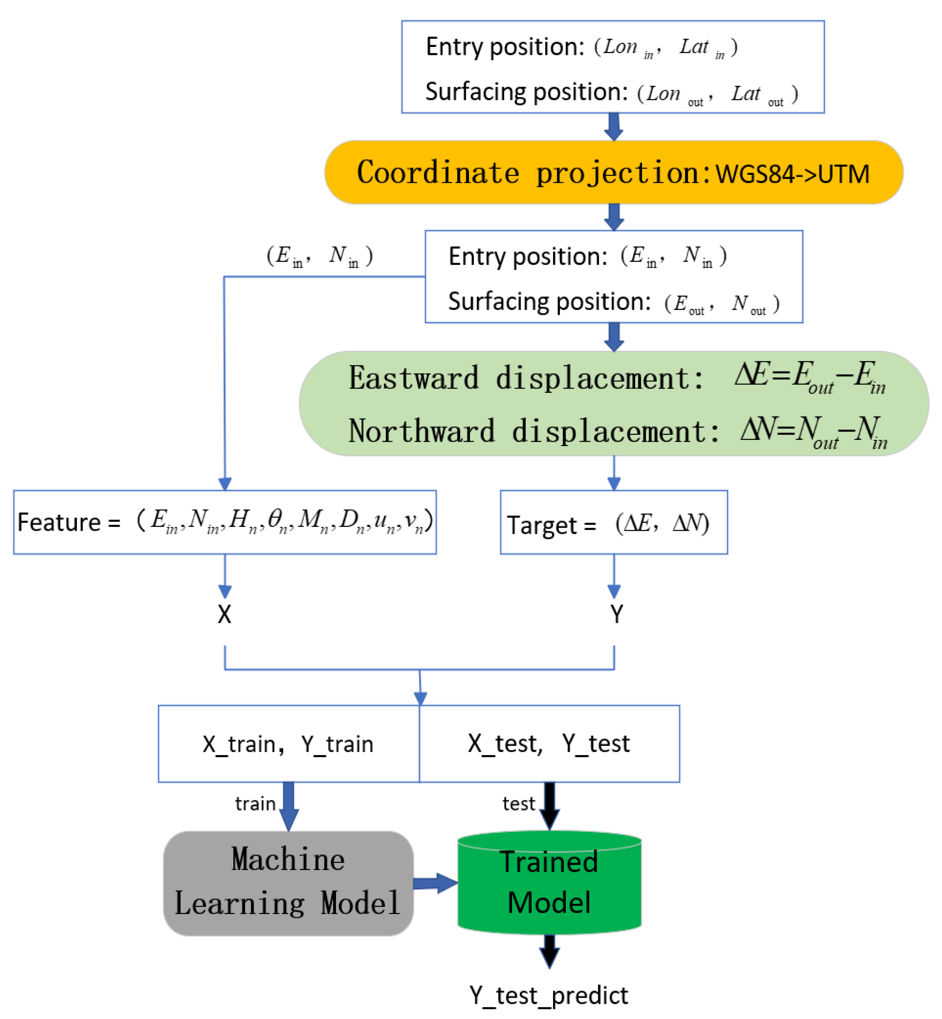
In early predictions of the surfacing position of underwater gliders, most approaches either performed regression directly in geographic coordinates (latitude and longitude) or relied on complex physical modeling of ocean currents. These methods often require precise estimates of ocean currents, and latitude and longitude still exhibit nonlinearity over small ranges. In other fields (such as ship trajectories or autonomous driving), considerable research has been conducted using UTM projection to simplify geographic distortion and combine it with machine learning for displacement prediction. However, there is still a lack of systematic validation and practical application in predicting the surfacing position of underwater gliders. Therefore, this paper applies the “coordinate transformation + data-driven prediction” approach for the first time in the context of glider surfacing position prediction, making corresponding improvements by considering the weak driving characteristics of underwater gliders and the features of profile data, as illustrated in Figure 1.

For ocean areas on the scale of tens of kilometers, converting latitude and longitude to the UTM coordinate system can reduce geographic nonlinear distortion and facilitate regression in meters. In each profile, assuming that the entry position $(E_{in},N_{in})$ and the surfacing position $(E_{out},N_{out})$ of the glider correspond to the transformed UTM coordinates, we define

$$\begin{array}{c}\Delta E=E_{out}-E_{in}\end{array}$$

(1)

$$\begin{array}{c}\Delta N=N_{out}-N_{in}\end{array}$$

(2)

where $\Delta E$ and $\Delta N$ represent the eastward and northward displacements of the glider for a profile, respectively. By taking $(\Delta E,\Delta N)$ as the prediction targets, we can avoid the coordinate distortion associated with directly regressing latitude and longitude.

In the existing literature on fields like shipping and autonomous vehicles (e.g., [18,19,20,21]), researchers often employ deep learning to regress the displacement of projected coordinates. In contrast, while this paper continues the overarching approach of “coordinate projection + regression to predict displacement”, it does not directly apply the deep learning framework. Instead, considering the weak driving characteristics of underwater gliders and the limited data scale, we have selected relatively lightweight and efficient machine learning algorithms such as AdaBoost, LGBM, and random forest. The specific process is as follows:

1.

Training Phase

Based on the previous steps, we obtain the entry position and motion displacement in the UTM coordinate system. Then, the transformed entry position is combined with the control parameters and ocean current velocities mentioned in Section 3.1 to form the input features, with the motion displacement as the prediction target. Machine learning algorithms are used for regression training.

2.

Prediction Phase

When the new profile entry coordinates are provided, they are combined with other feature data and input into the trained model to predict the displacement. Finally, the predicted displacement is added back to the UTM coordinates of the entry point and then converted back to geographic coordinates to obtain the predicted latitude and longitude of the surfacing point.

The implementation was carried out in Python (version 3.10) within the PyCharm 2023.1 Community Edition environment.

Through the above steps, this paper continues the approach of “coordinate projection + displacement regression” without using deep networks, achieving a balance between prediction accuracy and implementation simplicity. The following sections will combine actual sea trial data to further validate the effectiveness and applicability of this method.

3.3. Hyperparameter Selection

In this study, we employed five machine learning models and carefully selected their respective hyperparameters.

Taking the RF model as an example, max_depth indicates the maximum depth of the tree, and the max_features parameter controls the number of features that can be used for each decision tree at each split. n_estimators represents the number of base estimators, and its selection and quantity directly affect the model’s performance and computational efficiency. Increasing the number of base estimators typically improves model accuracy but also increases computational overhead. Therefore, selecting appropriate base estimators and their quantity is an important hyperparameter tuning task in practice.

A base estimator refers to the basic model or algorithm used in ensemble learning. These models can be various types of machine learning algorithms, such as decision trees, support vector machines, etc. The main idea of ensemble learning is to improve overall model performance and reduce the risk of overfitting by combining the predictions of multiple base learners. In this study, we use the decision tree model as the base learner for AdaBoost. And in

Table 2. Key parameters of the model used for direct latitude and longitude prediction in the first dataset.

Model	Parameter Value
	max_depth	max_features	n_estimators	learning_rate
DT	59	1.0	-	-
RF	400	1.0	100	-
AdaBoost	19	-	71	1.0
GB	4	-	217	0.188
LGBM	-	-	277	0.12

‘-’ denotes missing or unavailable parameters.

,

Table 3. Key parameters of the model used for displacement prediction based on coordinate transformation in the first dataset.

Model	Parameter Value
	max_depth	max_features	n_estimators	learning_rate
DT	49	0.86	-	-
RF	178	0.58	24	-
AdaBoost	12	-	56	0.948
GB	5	-	209	0.163
LGBM	-	-	97	0.168

‘-’ denotes missing or unavailable parameters.

,

Table 4. Key parameters of the model used for direct latitude and longitude prediction in the second dataset.

Model	Parameter Value
	max_depth	max_features	n_estimators	learning_rate
DT	100	1.0	-	-
RF	596	1.0	138	-
AdaBoost	21	-	300	0.99
GB	6	-	298	0.197
LGBM	-	-	26	0.032

‘-’ denotes missing or unavailable parameters.

and

Table 5. Key parameters of the model used for displacement prediction based on coordinate transformation in the second dataset.

Model	Parameter Value
	max_dept	max_features	n_estimators	learning_rate
DT	39	0.703	-	-
RF	132	0.565	26	-
AdaBoost	6	-	169	0.504
GB	3	-	65	0.137
LGBM	-	-	147	0.137

‘-’ denotes missing or unavailable parameters.

, the max_depth corresponding to ADA refers to the max_depth of the base learner it employs.

The learning_rate is an important hyperparameter in optimization algorithms that determines the step size at each parameter update. It plays a crucial role in training machine learning models, especially in neural networks and gradient descent methods. A learning rate that is too high may cause the model to oscillate around the optimal solution or even fail to converge, while a learning rate that is too low can slow down convergence, increase training time, and potentially lead to local optima. Therefore, selecting an appropriate learning rate is a critical factor in optimizing model performance.

We employed Bayesian optimization to adjust the model parameters in order to achieve optimal predictive performance. In Table 2 and Table 3, we provide the main parameters used for the first set of data when employing the direct latitude and longitude prediction method and the displacement prediction method based on coordinate transformation. In Table 4 and Table 5, we present the main parameters used for the second set of data when utilizing both methods.

3.4. Error Evaluation Criteria

In this study, to comprehensively evaluate the performance of each model in predicting the surfacing position of underwater gliders, we adopted five commonly used error evaluation criteria: MAE, RMSE, MAPE, Accuracy, and MDE. These metrics provide performance evaluations from different dimensions, allowing for a more comprehensive understanding of the model’s performance in practical applications. MAE serves as an intuitive indicator of the deviation between predicted and actual values. A lower MAE value indicates higher prediction accuracy of the model. The calculation formula for this metric is

$$MAE={\displaystyle \frac{1}{n}}\sum _{i=1}^n|y_i-{\widehat{y}}_i|$$

(3)

RMSE places greater weight on larger prediction errors by amplifying the errors’ squares, making it a strict metric. A lower RMSE indicates that the model performs well in overall data predictions, especially in handling potentially large errors. The calculation formula for this metric is

$$RMSE=\sqrt{{\displaystyle \frac{1}{n}}\sum _{i=1}^n{(y_i-{\widehat{y}}_i)}^2}$$

(4)

MAPE, usually expressed as a percentage, provides perspective on the size of the error relative to the actual value. A smaller MAPE indicates higher prediction accuracy. The calculation formula for this metric is

$$MAPE={\displaystyle \frac{1}{n}}\sum _{i=1}^n\left|{\displaystyle \frac{y_i-{\widehat{y}}_i}{y_i}}\right|\times 100$$

(5)

Accuracy indicates the proportion of correctly predicted samples to the total number of samples. The calculation formula for this metric is

$$ACCURACY={\displaystyle \frac{T}{T+F}}\times 100$$

(6)

Here, T represents the number of samples where the distance between the predicted exit position and the actual exit position is less than 500 m. F represents the number of samples where the distance between the predicted exit position and the actual exit position is greater than 500 m.

MDE is a metric for assessing the haversine distance error between predicted values and actual values. The calculation formula for this metric is

$$MDE={\displaystyle \frac{1}{n}}\sum _{i=1}^n\left|haversine(y_i,{\widehat{y}}_i)\right|$$

(7)

The selection of these metrics ensures that we can evaluate and compare the prediction performance of models from different angles, with each metric providing unique insights that enable us to assess the accuracy and reliability of the models in predicting surfacing positions in detail.

4. Results

This section presents a detailed evaluation of the proposed coordinate-transformation-based displacement prediction (CT) method versus the direct latitude–longitude prediction (LL) approach across two real-world underwater glider datasets. Both datasets are described in Section 3.1. In each dataset, 4/5 of the data is randomly selected as the training set, while the remaining 1/5 is used as the testing set. The training set is used to train the machine learning models, and the testing set is used to evaluate the results. The experiments adopt five commonly employed machine learning models (AdaBoost, LGBM, gradient boosting, random forest, and decision trees). We report results using the error metrics specified in Section 3.4 (MAE, RMSE, MAPE, Accuracy, and MDE), offering insights into the predictive performance and robustness of each approach.

Table 6. Prediction error of the surfacing position for the first dataset.

Model	AdaBoost	DT	GB	LGBM	RF
Method	LL/CT	LL/CT	LL/CT	LL/CT	LL/CT
MAE	0.009/0.0028	0.0125/0.0039	0.0154/0.0039	0.0074/0.0025	0.0086/0.0027
RMSE	0.015/0.004	0.0224/0.0058	0.0184/0.0052	0.0118/0.0037	0.0154/0.004
MAPE (%)	0.0053/0.0021	0.0074/0.003	0.0081/0.0027	0.004/0.0019	0.0052/0.0021
Accuracy (%)	21.578/64.965	13.689/48.724	0.696/43.619	25.522/68.213	28.074/67.517
MDE (km)	1.73/0.5	2.41/0.69	2.69/0.68	1.4/0.45	1.67/0.49

and

Table 7. Prediction error of the surfacing position for the second dataset.

Model	AdaBoost	DT	GB	LGBM	RF
Method	LL/CT	LL/CT	LL/CT	LL/CT	LL/CT
MAE	0.0067/0.0023	0.0085/0.0028	0.0055/0.0022	0.0108/0.0066	0.0066/0.0028
RMSE	0.0092/0.0031	0.012/0.0076	0.0076/0.0033	0.0163/0.0111	0.0094/0.0131
MAPE (%)	0.0066/0.0022	0.008/0.0025	0.0052/0.002	0.0118/0.0071	0.0064/0.0033
Accuracy (%)	19.931/72.852	13.402/73.196	25.773/74.914	1.375/21.306	19.588/83.162
MDE (km)	1.14/0.39	1.48/0.5	0.95/0.39	1.86/1.17	1.14/0.52

summarize the numerical outcomes. For visual clarity, we have bolded the CT results, while Figure 2, Figure 3, Figure 4 and Figure 5 illustrate representative predictions and error distributions. To make the prediction results more intuitive and the data visualization more appealing, we slice each predicted dataset by selecting 1 data point for display every 20 data points.

The remainder of this chapter is organized as follows: Section 4.1 explains the testing objectives and design approach; Section 4.2 discusses the prediction results from various aspects.

4.1. Testing Objectives and Design Approach

All experiments in this paper are based on real sea trial data, with the aim to comprehensively evaluate the differences and advantages of the proposed “displacement prediction method based on coordinate transformation” compared to the traditional “regression directly on latitude and longitude”. By testing on two sets of data collected from different marine areas, different glider platforms, and different time periods, we can assess the generalization ability and robustness of this method under actual sea conditions. Specifically, we perform the following:

1.

Validate the Effectiveness of Coordinate Transformation

In actual operations, glider routes often span long distances, and factors such as ocean currents, posture, and instrument accuracy can lead to cumulative errors. Converting latitude and longitude to UTM coordinates and performing regression solely on horizontal displacement can effectively mitigate geographic nonlinear distortions, thus validating the practicality of this approach in real marine environments.

2.

Compare the Performance of Multiple Models

Various common machine learning algorithms (such as AdaBoost and LGBM) will be selected for comparative experiments, which will not only test whether this method is dependent on specific models but also evaluate the adaptability of different algorithms under real sea conditions.

3.

Evaluate Accuracy and Stability

We have chosen multiple error metrics, including MAE, RMSE, and MAPE, and calculated the accuracy within a 500 m threshold to quantify the algorithm’s positioning accuracy and predictive stability under various environmental disturbances.

4.2. Discussion

This section discusses the “Coordinate Transformation Displacement Prediction (CT)” and “Direct Latitude-Longitude Regression (LL)” in terms of accuracy, stability, and practical applicability based on the experimental results. The discussion is as follows:

1.

Comparison of Prediction Accuracy

Table 6 lists the prediction errors for Dataset 1 (2159 samples), while Table 7 shows the results for Dataset 2 (1456 samples). In each case, we randomly split 80% of the data for training and the remaining 20% for testing; hence, the results reflect out-of-sample prediction capability. Notably, all five machine learning models consistently achieve lower MAE and RMSE under the CT strategy compared to LL-based predictions. For instance, in Table 6, the random forest (RF) model’s MAE drops from 0.0086 (LL) to 0.0027 (CT) in Dataset 1. A similar pattern is observed in Table 7, where the LGBM model’s MDE decreases from 1.86 km (LL) to 1.17 km (CT) in Dataset 2, indicating that the coordinate transformation framework effectively mitigates certain nonlinear effects inherent to raw latitude–longitude coordinates. Moreover, Accuracy (defined as the proportion of predictions within 500 m of the actual surfacing location) also exhibits significant improvements. In Table 6, the accuracy for RF on Dataset 1 increases from 28.074% (LL) to 67.517% (CT), demonstrating that more than 67% of the samples fall within the 500 m threshold once displacement-based prediction is employed. Such findings confirm that modeling displacement in the UTM system is advantageous for capturing small-scale spatial variations.

2.

Qualitative Analysis of Prediction Results

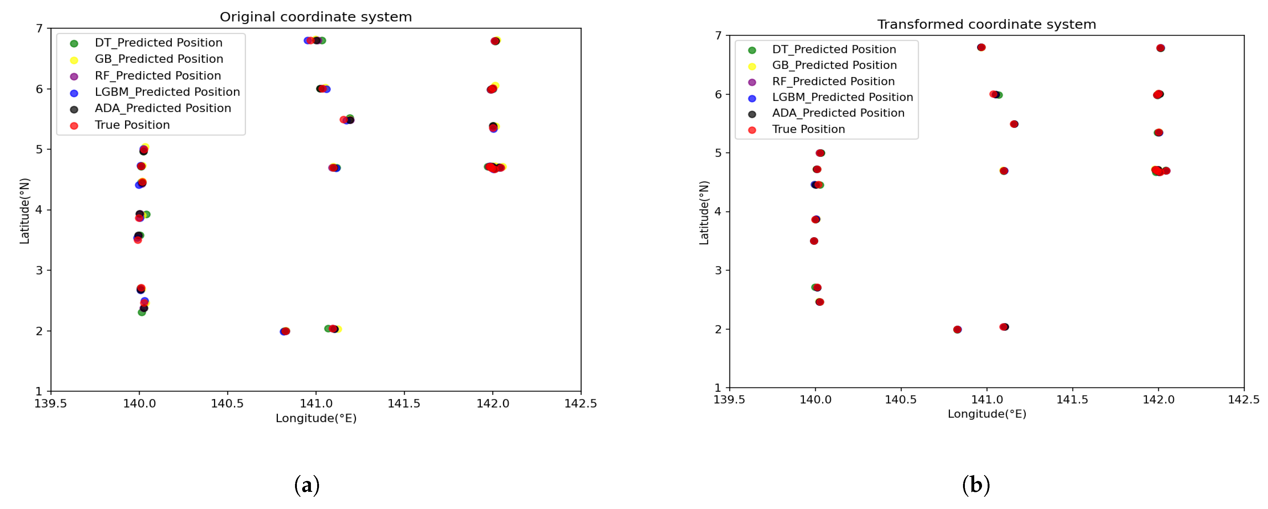
Figure 2 and Figure 3 illustrate the predicted surfacing positions in both LL and CT modes for Datasets 1 and 2, respectively. For clarity, only every 20th data point is plotted. In Figure 2a, predictions using LL coordinates tend to deviate more prominently from the true positions, especially in the middle portion of the trajectory. By contrast, in Figure 2b, the CT-based predictions exhibit trajectories that closely track the actual measured surfacing locations. This improvement can be attributed to the fact that UTM-based displacement simplifies positional shifts into near-linear relationships, thereby helping each model learn more consistent motion patterns. 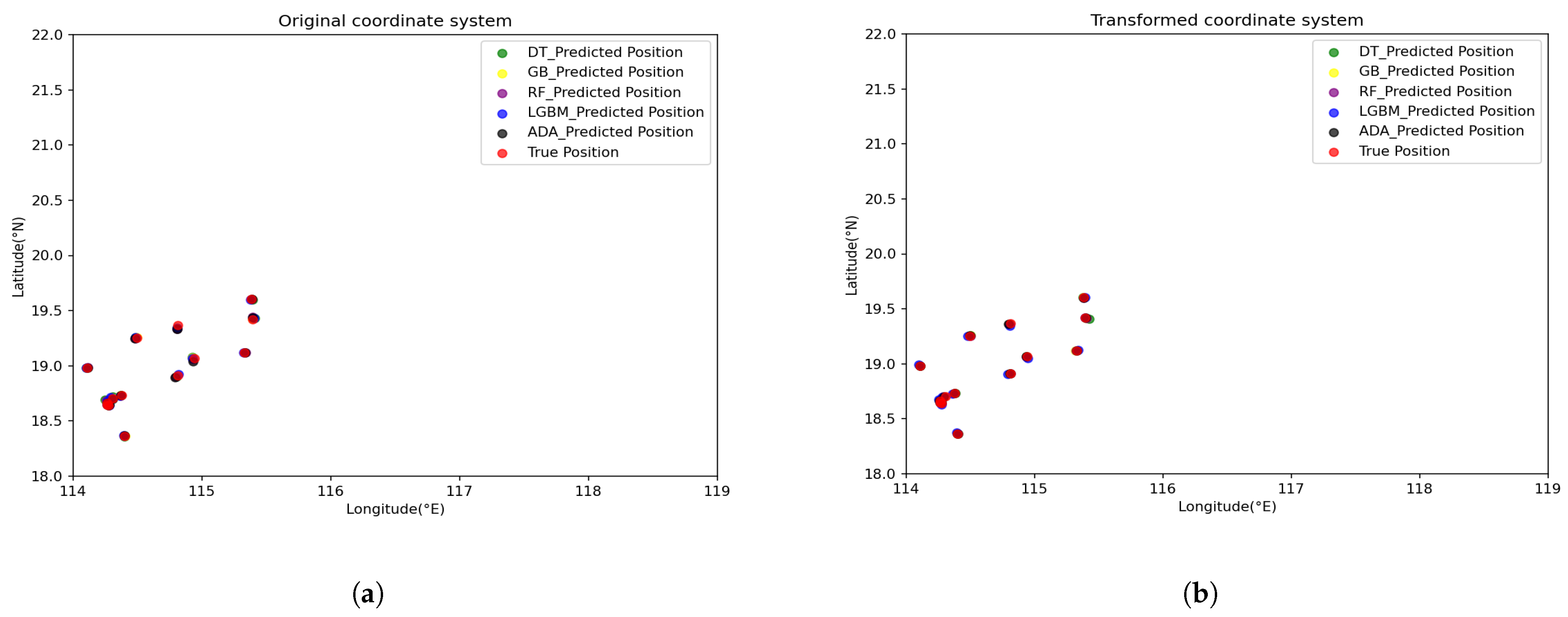Figure 3a,b present similar visual contrasts for Dataset 2. Notably, the AdaBoost and LGBM curves remain consistently near the ground truth in the CT setup (Figure 3b), whereas the LL-based approach (Figure 3a) shows larger mismatches and more variability. These qualitative observations align with the quantitative outcomes in Table 6 and Table 7, reinforcing the conclusion that CT-based displacement modeling generally improves surfacing position prediction.

3.

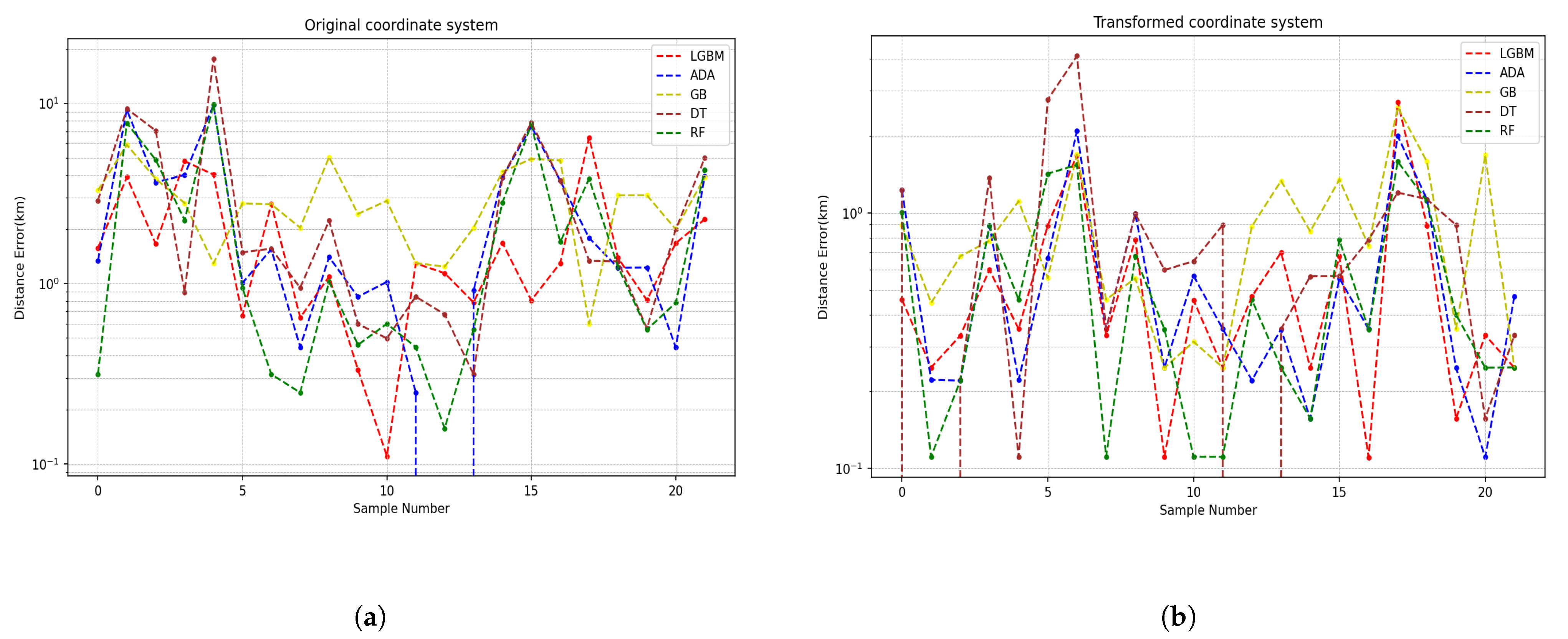
Error Distributions and Model Stability

To further investigate how errors are distributed across varying scales, Figure 4 and Figure 5 plot the log-scaled distance errors for each method. As shown in Figure 4a (Dataset 1), LL-based approaches exhibit broader error spreads, occasionally exceeding 2 km, whereas CT-based methods cluster more tightly at less than 1 km (Figure 4b). A similar trend is observed in Figure 5 for Dataset 2, highlighting that, even though certain outliers remain, the CT-based methods tend to compress the distribution of errors toward lower magnitudes. In particular, AdaBoost, DT, and GB demonstrate relatively stable performance for both datasets, while LGBM and random forest (RF) show somewhat greater fluctuation. Such patterns suggest that transforming coordinates to a planar system reduces the complexity of learning direct latitude–longitude relationships, thus enabling the data-driven models to better capture displacement trends. Additionally, the consistent performance across multiple algorithms indicates that the improvement is not strictly tied to a specific model type but rather to the coordinate transformation mechanism itself.

4.

Summary of Key Observations

In the study, we significantly improved the accuracy of predictions using the coordinate transformation (CT) method. In both datasets, all five models had notably lower errors (MAE, RMSE, and MDE) when predicting in the UTM displacement space compared to using raw latitude and longitude. In some cases (for example, using random forest on Dataset 1), the accuracy rate (within 500 m) can be doubled. Furthermore, the coordinate transformation method demonstrates consistent robustness across various learning algorithms (such as AdaBoost, LGBM, gradient boosting, random forest, and decision trees), indicating that the performance improvement primarily stems from the simplification of the coordinate space rather than the complexities of specific models. Log-scale error plots show that extreme error values (e.g., >2 km) are significantly reduced under the CT strategy, confirming that coordinate transformation diminishes the impact of geographic distortions in small operational areas. Although the transformation from WGS84 to UTM adds a preprocessing step, it is straightforward to implement using commonly available libraries (such as pyproj) and consistently yields better prediction accuracy, reflecting a favorable trade-off between preprocessing complexity and predictive performance.

5. Discussion

In this chapter, we undertake a deeper examination of the experimental results comparing the coordinate-transformation-based displacement prediction method (CT) and the direct latitude–longitude regression (LL). Section 5.1 discusses the experimental outcomes of both approaches, providing an in-depth analysis of their differences in prediction accuracy and stability. It also uses model error distributions to explore the strengths, weaknesses, and possible sources of error for each algorithm. Section 5.2 focuses on the practical significance of these findings and how to maximize the benefits of improved accuracy in real-world deployments, particularly in reducing sea-trial recovery efforts, operational costs, and reliance on multi-source ocean data. Section 5.3 shifts the perspective to error analysis and contrasts model performance under different sea conditions or profile circumstances. It summarizes potential environmental and model-related factors leading to prediction errors and proposes possible strategies for mitigating those errors.

5.1. Comparison of Prediction Methods (CT vs. Direct LL)

Our experiments clearly show that the coordinate transformation (CT) approach outperforms direct latitude–longitude (LL) prediction across all tested models. In both datasets, using CT drastically improved accuracy (percentage of predictions within 500 m of true surfacing location) and reduced error metrics relative to the LL method. For example, in Dataset 1 the random forest model’s accuracy roughly doubled from about 28% with direct LL to 67.5% with CT, and in Dataset 2 it jumped from 19.6% to 83.2%. Similar gains were observed for other models (AdaBoost, gradient boosting, etc.), with CT often boosting accuracy by factors of 2–4. These results underscore that projecting positions into a planar coordinate system (UTM) makes the prediction task easier for learning algorithms. By contrast, models trained directly on geodetic coordinates struggled to achieve high accuracy—in some cases yielding <20–30% accuracy—indicating their difficulty in learning the nonlinear relationship between input features and the glider’s surfacing point in raw latitude–longitude space.

The superior performance of CT can be explained by the geometric simplification it provides. Latitude and longitude values change nonlinearly with position and suffer from distortion over even small areas. In other words, a given linear distance in one part of the region does not correspond to the same change in lat/long in another part, which makes it hard for machine learning models to learn consistent patterns. Additionally, using raw lat/long means that the model has to implicitly account for the Earth’s curvature; the angular measurements can introduce errors if treated in a Cartesian way. These factors lead to complex, nonlinear relationships that data-driven models find hard to capture. The CT method addresses this by converting geographic coordinates into a Universal Transverse Mercator plane, where distance relationships are more linear and uniform. In our approach, the glider’s dive and surfacing coordinates are transformed to UTM; the model then predicts the displacement in this planar space, which is essentially a linear “residual” vector, and finally the prediction is converted back to latitude–longitude. This way, the model only needs to learn a relatively straightforward mapping in a Euclidean space, avoiding the highly nonlinear mapping of raw coordinates. The result is a notable boost in predictive accuracy and robustness for all models. For instance, without CT, even advanced models often missed the surfacing point by over 500 m (yielding low accuracy percentages), whereas with CT, most predictions fell well below that threshold (reflected in much higher accuracy percentages). We also saw that CT greatly shrinks extreme errors: the worst-case surfacing location errors (outliers of 1–2 km) observed with direct LL were largely eliminated under CT.

Another important observation is that this performance gain from CT was consistent regardless of the complexity of the model. Both simple models (e.g., a single decision tree) and more sophisticated ensemble methods benefited from the coordinate transformation to a similar degree. This suggests that it is the feature space transformation driving the improvement, rather than any particular tuning of a complex model. In fact, even the simplest model tested (decision tree) with CT outperformed more complex models using raw coordinates, highlighting how much easier the learning problem becomes after removing geographic distortions. The CT approach thus provides a strong “foundation” that allows even basic algorithms to achieve high accuracy. It is also worth noting that the added preprocessing step is minimal: conversion between WGS84 lat/long and UTM can be performed with standard libraries (e.g., pyproj in Python) and involves negligible computational cost. This small overhead is well justified by the accuracy gains: a favorable trade-off between preprocessing complexity and predictive performance. In summary, the CT method proved to be a consistently better approach for surfacing position prediction, effectively handling issues of nonlinearity and scale that handicap the direct LL method.

5.2. Error Analysis

Although all models improved with coordinate transformation, their relative performance varied between scenarios, indicating that certain models are better suited for specific conditions. Overall, ensemble methods tended to perform more reliably than a single decision tree. AdaBoost exhibited the most robust performance across both datasets, emerging as the best overall model in terms of low error and high accuracy. For instance, AdaBoost achieved 72.9% accuracy in Dataset 2 (within 500 m)—one of the highest scores—and maintained low mean errors in both cases. Random forest was similarly strong, particularly excelling in Dataset 2 (over 83% accuracy). In contrast, the standalone decision tree model had more variable results: in the more complex environment of Dataset 1, it only reached 48.7% accuracy (significantly lower than any ensemble), indicating it underfit the intricacies of that scenario. Interestingly, in Dataset 2, even the single tree’s accuracy ( 73.2%) was on par with AdaBoost, suggesting that the underlying pattern in that dataset was simpler or more linear, allowing a simple model to capture it. This reveals that scenario complexity plays a role: when the mapping from inputs to surfacing displacement is relatively straightforward (perhaps due to more consistent ocean currents or shorter distances), simpler models can suffice, whereas more complex conditions benefit from ensemble learning.

We also observed some anomalies that warrant analysis. The LightGBM (LGBM) model, for example, had inconsistent performance between the two datasets. In Dataset 1, LGBM with CT was among the top performers (≈68% accuracy), but in Dataset 2 its accuracy with CT dropped to only 21%, far below the other models. This poor outcome in the second scenario suggests LGBM might have been more sensitive to the training data characteristics or noise. One possibility is that LGBM overfit some spurious patterns in the smaller Dataset 2 (which had fewer samples) or struggled with the higher proportion of invalid/missing current readings in that dataset. A telltale sign is the much larger mean distance error for LGBM: even after CT, its average prediction error in Dataset 2 was about 1.17 km, compared to 0.3–0.5 km for the other methods. This implies LGBM had a few significant outlier errors (e.g., predicting a surfacing point off by >1 km), drastically reducing its within-500 m accuracy. In contrast, AdaBoost and random forest seem to have generalized better and avoided such large mistakes in that same scenario. This difference may come down to how each algorithm handles variance and outliers: random forest averages many decorrelated trees, which can smooth out odd predictions, and AdaBoost, by reweighting errors, can be robust if its base learners focus on the more common patterns. LGBM (and the other gradient boosting implementation) might have zeroed in on a particular feature combination that coincidentally led to a big error on certain test cases. These findings highlight the need for careful model tuning and validation in each deployment scenario; an algorithm that is best in one region or dataset might not be universally best without adjustment.

Beyond model choice, it is important to consider broader sources of prediction error. The results and error distributions of Table 6 and Table 7 indicate that most residual errors after CT are on the order of a few hundred meters, but some outliers remain. Key factors contributing to these prediction errors likely include the following:

1.

Environmental variability

Unmodeled changes in ocean currents or turbulence between the glider’s dive and surfacing can introduce errors. Our features included depth-averaged current estimates, but these may not capture sudden shifts or vertical current shear that the glider experiences. For instance, if a glider encounters an unforeseen lateral current pulse, the actual surfacing point could deviate beyond what the model expected based on past averages. Such unpredictable ocean dynamics set a limit on attainable accuracy for any purely data-driven model.

2.

Sensor and input noise

Small errors in measuring or recording the input features (e.g., the glider’s heading, pitch, or the depth-averaged current) will propagate to the prediction. If the compass or inertial navigation on the glider has drift, the input position and heading may be off, leading the model to predict a slightly incorrect displacement. Similarly, the current estimates provided to the model might be noisy (especially if “−1” or “1” were used to flag invalid data and not perfectly filtered out), which could mislead the prediction for that profile.

3.

Model limitations

Even with CT, the machine learning models have finite capacity and were trained on finite data. They may struggle with profiles that fall outside the training distribution. For example, a very atypical combination of dive angle, buoyancy, and current that was not seen before could yield a larger error. A single decision tree is especially prone to erratic predictions if a test sample follows a path in the tree that was supported by few training data. Ensemble methods mitigate this but can still err if the underlying signal is weak. Additionally, our models treated each dive-surfacing cycle independently; any temporal dependencies (e.g., slowly varying currents) had to be inferred indirectly, so sudden regime changes could lead to errors until the model “catches up” in retraining.

To mitigate these errors, several strategies can be considered. First, improving data quality and feature engineering can help: for instance, filtering or interpolating any missing/invalid current readings would give the models more reliable inputs, and incorporating additional sensors (if available), like an onboard Doppler velocity log or a wave height estimate, could account for factors that are currently unmodeled. Second, one could use an ensemble of prediction models and cross-check their outputs; if one model (say, LGBM) predicts an outlier location while others cluster elsewhere, the system could flag low confidence in that prediction and default to a more robust method. Another mitigation approach is imposing physical constraints or bias correction. Since we know a priori that the glider cannot stray beyond a certain distance given its speed and dive duration, an extremely large predicted displacement could be adjusted or bounded. Likewise, if a particular glider consistently shows a bias (like always undershooting eastward displacement due to unmodeled currents), a simple linear bias correction could be applied to the predictions. Lastly, continued retraining and model adaptation with new data will reduce errors: as the glider conducts more missions in an area, the model can be updated to learn any new patterns (for example, seasonal changes in current), thereby continuously refining the predictive accuracy. If the operational area expands, an adaptive strategy might involve partitioning the area into smaller zones and applying separate coordinate transformations or models in each to maintain the assumption of locally linear displacements and avoid projection error buildup. Indeed, our findings indicated that, for regions on the order of tens of kilometers, a single UTM projection was effective and introduced negligible error, but for substantially larger expanses, using multiple local coordinate frames could be a prudent way to keep errors low.

5.3. Implications of Results

The improvements in prediction accuracy demonstrated by the CT approach carry significant practical implications for underwater glider operations. High-precision surfacing point forecasts translate directly into more efficient and reliable glider recovery. In field operations, knowing the surfacing location within a few hundred meters means a recovery vessel can plan its approach much more precisely, saving time and fuel that would otherwise be spent searching a wide area. For example, reducing the typical surfacing error from about 1–2 km down to 0.3–0.5 km effectively shrinks the search circle to less than a tenth of its original area. This can cut down on retrieval efforts and costs substantially, especially when managing fleets of gliders. Moreover, improved accuracy enhances mission safety: the glider is less likely to drift into hazardous areas (rocky coastlines, shipping lanes) unexpectedly, and if it does, the operators have a precise prediction to act upon (e.g., dispatching recovery before it reaches danger). In scenarios where multiple gliders or AUVs are deployed, high prediction accuracy also facilitates coordination and tracking, as each vehicle’s position can be anticipated with confidence.

A key advantage of our method is its minimal reliance on external oceanographic data. Many state-of-the-art approaches for predicting AUV/UG trajectories incorporate outputs from regional ocean models, satellite data, or multi-sensor data streams to account for currents and environmental forces. While effective, those multi-source approaches increase operational complexity and may not always be feasible in real time or in every location. In contrast, our CT-based prediction uses only the glider’s internally recorded metrics (past position, heading, dive parameters, and a depth-averaged current estimate derived from the glider’s drift) and achieves comparable or better accuracy without needing dense ocean model inputs. The reduced dependency on multi-source data has several benefits for real-world deployment:

1.

Deployable in data-sparse regions

The glider can be sent to remote areas where we lack detailed ocean model coverage or live data feeds. The prediction framework will still function because it learns from the glider’s own measurements. This autonomy is crucial for long-duration missions in the open ocean or under-ice deployments where external data access is limited.

2.

Lower operational overhead

There is no need to gather, transmit, and process large volumes of environmental data for input. This simplifies the support infrastructure and reduces communication requirements (which is important if the glider has limited bandwidth to shore). For instance, we avoid having to continuously update the glider with ocean current forecasts from a remote server.

3.

Robustness to model errors

Relying on complex ocean models can introduce failure points if those models are inaccurate or misaligned with local conditions. By not depending on them, our method circumvents this issue: it learns the effective ocean influence directly from the glider’s movement. This means that if the actual currents deviate from climatology or forecasts, our predictor can still adapt (given enough training data from that environment). In essence, the glider’s own experience feeds the prediction, making it self-contained and adaptive to the local ocean dynamics.

Furthermore, the CT approach’s strong performance with simpler machine learning models makes it well-suited for real-time or onboard implementation. Since it does not require heavy computation, a glider’s onboard computer or a lightweight field laptop could run the prediction algorithm to estimate the surfacing point before the glider actually surfaces. This opens up possibilities for closed-loop operational strategies, for example, if a predicted surfacing point is too close to a hazard, the glider (or operators) could be alerted in advance to adjust course or terminate the dive early. The robust accuracy we achieved means such decisions can be made confidently, improving the glider’s autonomous capabilities. Overall, these results demonstrate a significant step towards more cost-effective and reliable glider missions, where high precision is achieved with elegant simplifications instead of complex data requirements.

6. Conclusions

In this section, we summarize the theoretical contributions, practical significance, limitations, and future work of this paper, and we also introduce the machine learning model that achieved the lowest prediction error. The specific content is as follows:

1.

Theoretical Contributions

This study advances the understanding of underwater glider surfacing position prediction by reframing the problem through a coordinate transformation approach. Instead of predicting geographic latitude–longitude coordinates directly, positions are projected into a planar Universal Transverse Mercator (UTM) coordinate system and the surfacing displacement vector is predicted, effectively overcoming the nonlinear challenges of direct latitude–longitude regression. This novel application of coordinate transformations (introduced here for the first time in the underwater glider domain) enables machine learning models to capture motion patterns more consistently, as the UTM-based displacement simplifies spatial relationships into a near-linear form that is easier to learn. As a result, the proposed framework demonstrates that changing the coordinate frame can substantially improve predictive performance without relying on complex, multi-source ocean current models. These contributions deepen the theoretical insight into surfacing position prediction, highlighting the impact of coordinate framing on model accuracy in marine navigation contexts.

2.

Practical Significance

Practically, the coordinate transformation method yields notable improvements in prediction accuracy while reducing dependence on extensive oceanographic data. Experiments on two real-world sea trial datasets showed that this approach can improve surfacing position accuracy by up to 50% within a 500 m range compared to direct latitude–longitude regression, all with minimal reliance on multi-source ocean data. By employing relatively simple machine learning models (e.g., decision trees and boosting ensembles) instead of complex deep learning architectures, the method also runs with lower computational overhead. These efficiencies make the approach well-suited for resource-constrained environments, such as on-board glider systems with limited processing power or missions where detailed ocean current inputs are unavailable, all without sacrificing predictive precision. In summary, the proposed solution offers a more cost-effective and data-efficient strategy for high-precision glider navigation.

3.

Best Performing Model

Among the machine learning models evaluated, AdaBoost emerged as the best-performing model, achieving the highest predictive accuracy and lowest error rates across both datasets. For instance, on the second dataset AdaBoost attained a mean absolute error of approximately 0.0023 (in transformed UTM coordinates), which was significantly lower than that of the other algorithms, and even improved upon its own performance from the first dataset. AdaBoost also achieved the highest accuracy in terms of geospatial precision, with about 72.85% of predicted surfacing locations falling within 500 m of the true position in Dataset 2. This outpaced models like random forest, LightGBM, and gradient boosting, underscoring AdaBoost’s strength in capturing the glider’s nonlinear displacement patterns. The superior performance of AdaBoost can be attributed to its ensemble learning mechanism, which combines multiple weak learners to better generalize the underlying motion dynamics, giving it a distinct advantage over the other models in this study.

4.

Limitations

Despite the promising results, several limitations of this study should be acknowledged. First, the models were developed and tested on a limited set of sea trial datasets, which may not encompass the full spectrum of environmental variability (such as different current regimes, wave conditions, and seafloor topographies) that underwater gliders can encounter. These environmental factors were not explicitly incorporated into the prediction features, so the model’s performance could degrade if deployed in conditions that diverge significantly from those seen in training. Second, the scope of this work was restricted to conventional machine learning algorithms, and we did not evaluate more complex approaches like deep learning or hybrid physics–ML models; this leaves open the possibility that advanced models might further improve prediction accuracy. These constraints imply that caution is needed in generalizing the findings; the current model’s generalizability to different regions, seasons, or extreme ocean conditions remains unproven. Overall, additional validation with more diverse data and scenarios is necessary to fully establish the robustness of the proposed method.

5.

Future Work

Building on this research, several avenues for future work are suggested. One direction is to integrate advanced deep learning techniques to capture more complex spatiotemporal patterns in glider dynamics: for example, multi-modal neural networks with attention mechanisms could be employed to fuse various data sources and potentially uncover synergies between the coordinate transformation approach and learned representations. Another important extension is to incorporate richer environmental and contextual features into the model—such as real-time current measurements, wave state information, or other oceanographic data—to enhance the model’s robustness and adaptability across diverse operational conditions. Additionally, conducting real-world deployment trials with underwater gliders would be valuable to evaluate the approach in operational settings. Such field experiments can provide insight into the method’s performance over prolonged missions and help identify practical issues (e.g., onboard computational constraints or integration with glider control systems), guiding further refinements. By pursuing these directions, future research can further improve surfacing position prediction and facilitate the transition of this technique from simulation to reliable field deployment.