
Spatio-Temporal Prediction of Surface Remote Sensing Data in Equatorial Pacific Ocean Based on Multi-Element Fusion Network


Abstract
1. Introduction
- (1)
- A multi-element fusion network model based on ConvLSTM and an attention mechanism is proposed, which includes the multi-element input layer, 3D convolutional layer, attention fusion layer, ConvLSTM layer, and single-element prediction output layer. The 3D convolution can better extract the spatio-temporal information of the elements, and the attentional mechanism can fuse the hidden features of multiple elements in the prediction of the SST, and the use of encoding and decoding ConvLSTM enables the spatio-temporal features of the SST to be better learned.
- (2)
- Prediction accuracy experiments with multiple-element inputs and feature fusion were designed to analyze the effects of different elemental inputs on the prediction performance of the multi-element fusion model using the prediction results. A comparative analysis with other benchmark model prediction results was also conducted to evaluate the model performance according to different indicators.
- (3)
- The prediction effect of the multi-element fusion network model for the equatorial Pacific Ocean was analyzed, and the prediction ability of the model for the SST in El Niño and La Niña years was verified.
2. Methods and Models
2.1. Multi-Element Data Sources
2.2. Methods
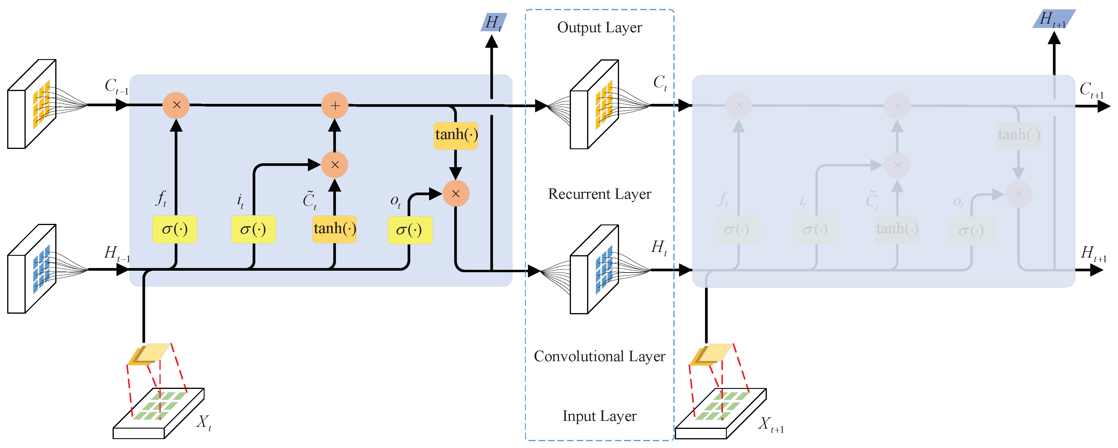
2.2.1. ConvLSTM Network
2.2.2. Correlation Analysis of Multiple-Source Marine Environmental Elements
2.2.3. Multi-Element Fusion Network Model
- (1)
- Multi-Element Input Layer:The types of multi-element input include the SST, SLA and SSW. Firstly, the multi-element data are subjected to a maximum–minimum normalization process to standardize the multi-element data, eliminate the order-of-magnitude differences between various marine environmental element data due to the differences in numerical ranges and units of measurement and scale the data to a reasonable range of intervals so as to improve the training efficiency and make it easier for the model to converge. The normalization process equation is as follows:where is the data in the interval [0, 1] after normalization, and are the maximum and minimum values of the original data in the region and is the original data.Finally, the normalized data are fed into the 3D convolutional layer. The input shapes of the SST, SLA and SSW are denoted by (None, timesteps, rows, cols, 1), where None, timesteps, rows, cols and 1 denote the number of samples, the input timestep, the rows of the data matrix, the columns of the data matrix and the number of channels.
- (2)
- 3D Convolutional Layer:The function of the 3D convolutional layer is to extract the hidden temporal and spatial information of the elements by using Conv3D units. A Conv3D unit is a 3-dimensional convolution process, which completes the convolution kernels and the element values at the corresponding position obtained by first multiplying the product before summation, by moving the 3 × 3 × 3 convolution kernels in the 2-dimensional image plane and the 3rd-dimensional depth direction. Table 2 shows the parameter settings of Conv3D, and a 3-dimensional convolution operation is performed for each of the 3 elements, using 40 filters, so the data shape is (None, timesteps, rows, cols, 40).
- (3)
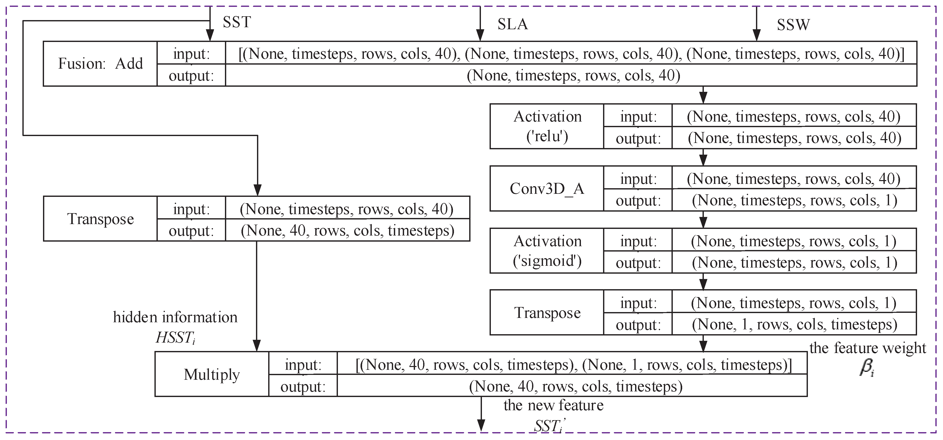
- Attention Fusion Layer:The attention fusion layer mainly utilizes the attention mechanism to fuse the correlated features among the three multi-elements of the SST, SLA and SSW and reassign feature weights to the predicted SST elements to generate new weighted features. In this case, the attention mechanism assigns different weights to all input feature sequences, and the different feature attention weights are jointly determined by the degree of correlation between the model input features and the network output. During the training process, the attention mechanism continuously matches important information with higher weights and filters out invalid information that can be ignored with lower weights. As the training times accumulate, the attention weight matrix used for information matching is continuously optimized, and the trained neural network parameters become more usable.This workflow is divided into two parts, as shown in Figure 4. In one part, hidden information about the SST, , is obtained using the Transpose unit. In the other part, the feature weight of multiple elements (SST, SLA and SSW) is obtained through the continuous use of the Add, ReLU, Conv3D_A, Sigmoid and Transpose units, where Table 2 shows the functional description and parameter settings of the module units. Finally, and are multiplied to obtain the new feature ’, the data shape of which is (None, 40, rows, cols, timesteps).
- (4)
- ConvLSTM Layer:The function of the ConvLSTM layer is to further extract features, and it mainly captures long time sequence dependencies, augments the time taken to generate target lengths and remembers and stores information. The structure of the ConvLSTM layer is shown in Figure 3, and the functional description and parameter settings are shown in Table 2. The output is obtained through the continuous application of the Transpose, 2 ConvLSTM 2D, Conversion and 2 ConvLSTM 2D units, and the data shape is (None, targetsizes, rows, cols, 32).
- (5)
- Single-Element Prediction Output Layer:The fully connected layer maps the extracted features to the output space using a nonlinear transformation and then visualizes the prediction results through inverse normalization. The inverse normalization equation is as follows:where the symbolic interpretation is the same as in Equation (7), and is the visualization of the true prediction at each position, i, in the [rows, cols] region. The shape of the output prediction result is represented by (1, targetsizes, rows, cols, 1), where targetsizes represent the number of days directly predicted for the output.
2.3. Evaluation Indicators
3. Results
3.1. Prediction Accuracy Experiments with Multi-Element Input and Feature Fusion
- (1)
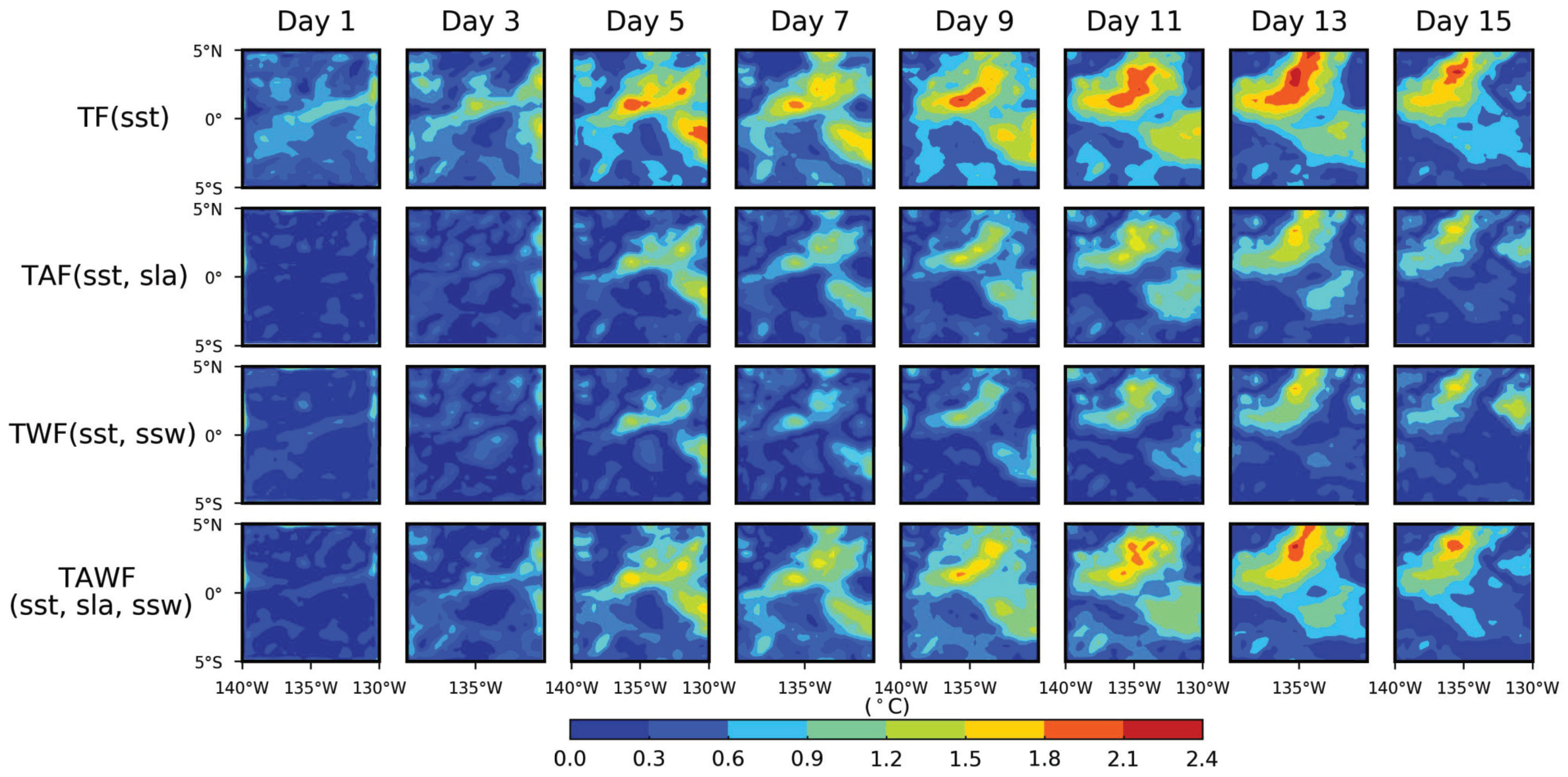
- TF(sst): Input the SST and predict the output SST.
- (2)
- TAF(sst, sla): Input the SST and SLA and predict the output SST.
- (3)
- TWF(sst, ssw): Input the SST and SSW and predict the output SST.
- (4)
- TAWF(sst, sla, ssw): Input the SST, SLA and SSW and predict the output SST.
3.1.1. Experiments on Analyzing Historical Input Lengths and Predicted Output Lengths
3.1.2. Experiments on Analyzing Multi-Element Fusion Methods Under Different Element Inputs
- (1)
- Location A: In Figure 5, the location with the highest real SST in the real 1-day data.
- (2)
- Location B: In Figure 5, the location with the lowest real SST in the real 1-day data.
- (3)
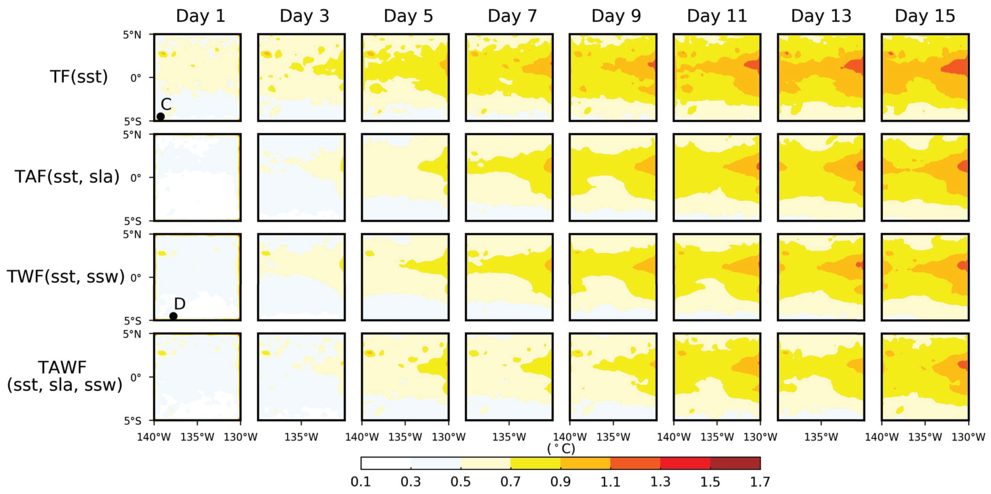
- Location C: In Figure 7, the location with the smallest Poi_RMSE in the 1-day TF(sst) model.
- (4)
- Location D: In Figure 7, the location with the smallest Poi_RMSE in the 1-day TWF(sst, ssw) model.
3.2. Comparative Analysis with Other Model Prediction Results
- (1)
- Multi-Channel LSTM [38]: The encoder and decoder are built using two LSTM layers, respectively, and depending on the elements of the multi-channel inputs, we can obtain LSTM and Multi-LSTM.
- (2)
- Multi-Channel ATT-LSTM: By introducing an attention mechanism to a multi-channel LSTM foundation, the corresponding ATT-LSTM and Multi-ATT-LSTM models can be obtained.
- (3)
- ConvLSTM [37]: Using a single-element model with only an SST input and two ConvLSTM2D layers to build an encoder and decoder, respectively, we can obtain ConvLSTM. We can also obtain CNN+ConvLSTM by adding a CNN layer.
- (4)
- ATT-ConvLSTM [43]: A channel attention mechanism is introduced to fuse multi-element inputs based on ConvLSTM to obtain ATT-ConvLSTM-Fusion. It is worth noting that the channel attention mechanism is different from the attention mechanism used in the TWF(sst, ssw) model proposed in this paper.
- (5)
- LICOM [55]: The global ocean circulation model developed by the Institute of Atmospheric Physics of the Chinese Academy of Sciences is numerically solved using a finite difference method under the given initial and boundary values and is applied to short- and medium-term marine environmental forecasting.
3.3. Prediction Experiment for Equatorial Pacific Ocean
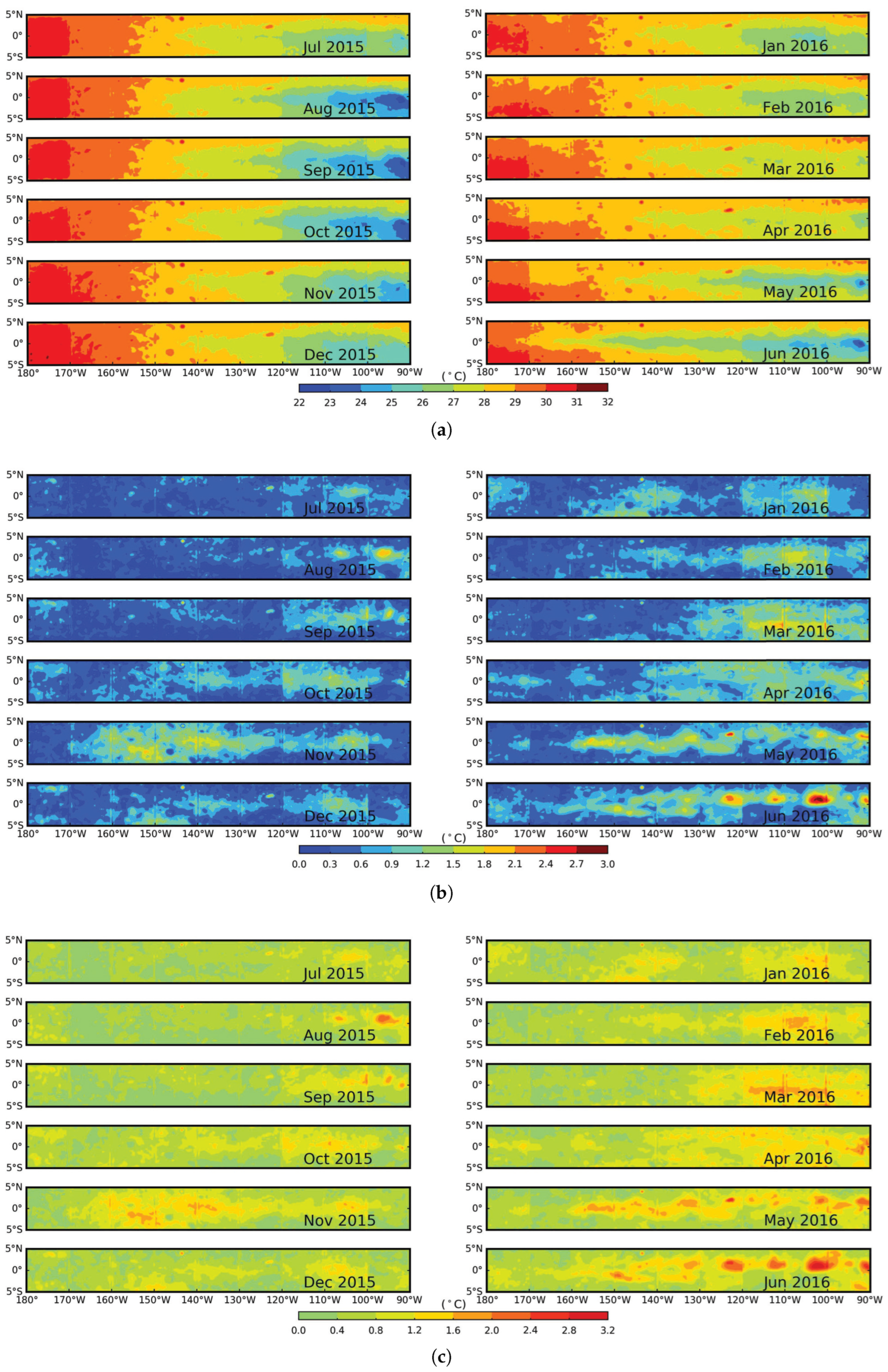
3.3.1. Prediction Experiments for the Equatorial Pacific Ocean in El Niño Years
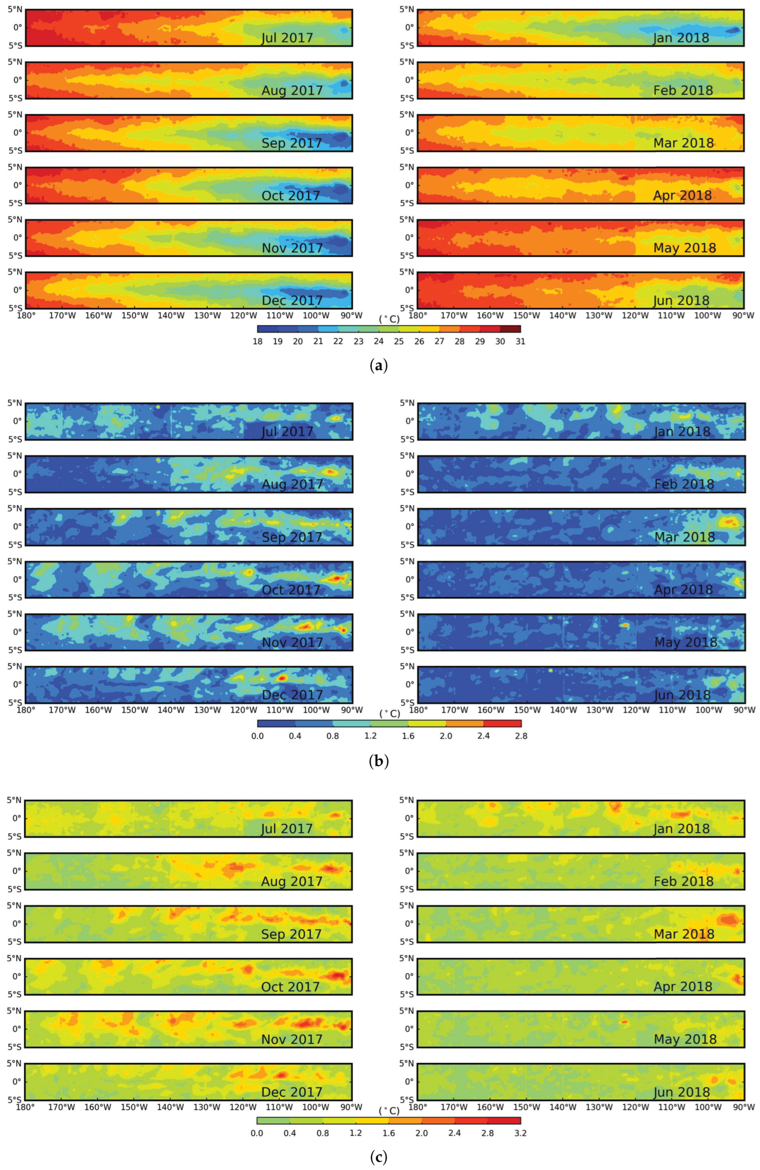
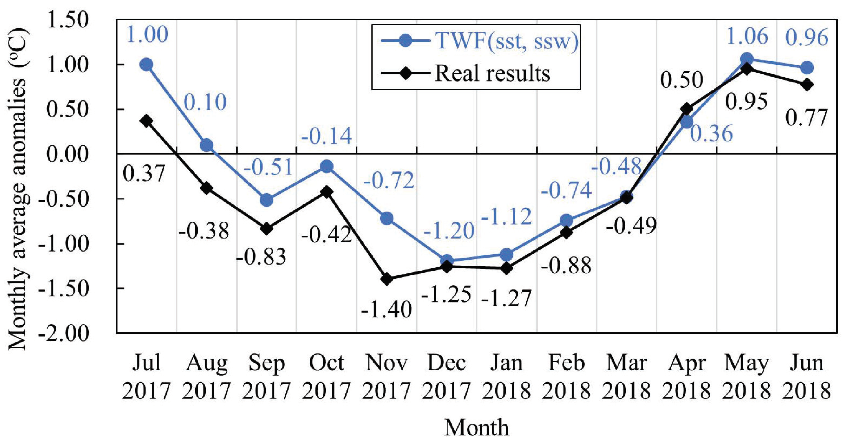
3.3.2. Prediction Experiments for the Equatorial Pacific Ocean in La Niña Years
4. Discussion
5. Conclusions
- (1)
- The accuracy of the model was evaluated using the RMSE and PACC. The TWF(sst, ssw) model had the smallest Reg_RMSE.mean of 0.4748 °C, and the results for the Reg_RMSE.mean were as follows: TF(sst) > TAWF(sst, sla, ssw) > TAF(sst, sla) > TWF(sst, ssw). The prediction accuracy of the model was affected by the multi-element inputs. The two-element fusion model using the SSW and SLA as the multi-element inputs had smaller prediction errors than the SST single-element model and even smaller prediction errors than the three-element fusion model. Here, the TWF(sst, ssw) model had the best prediction ability.
- (2)
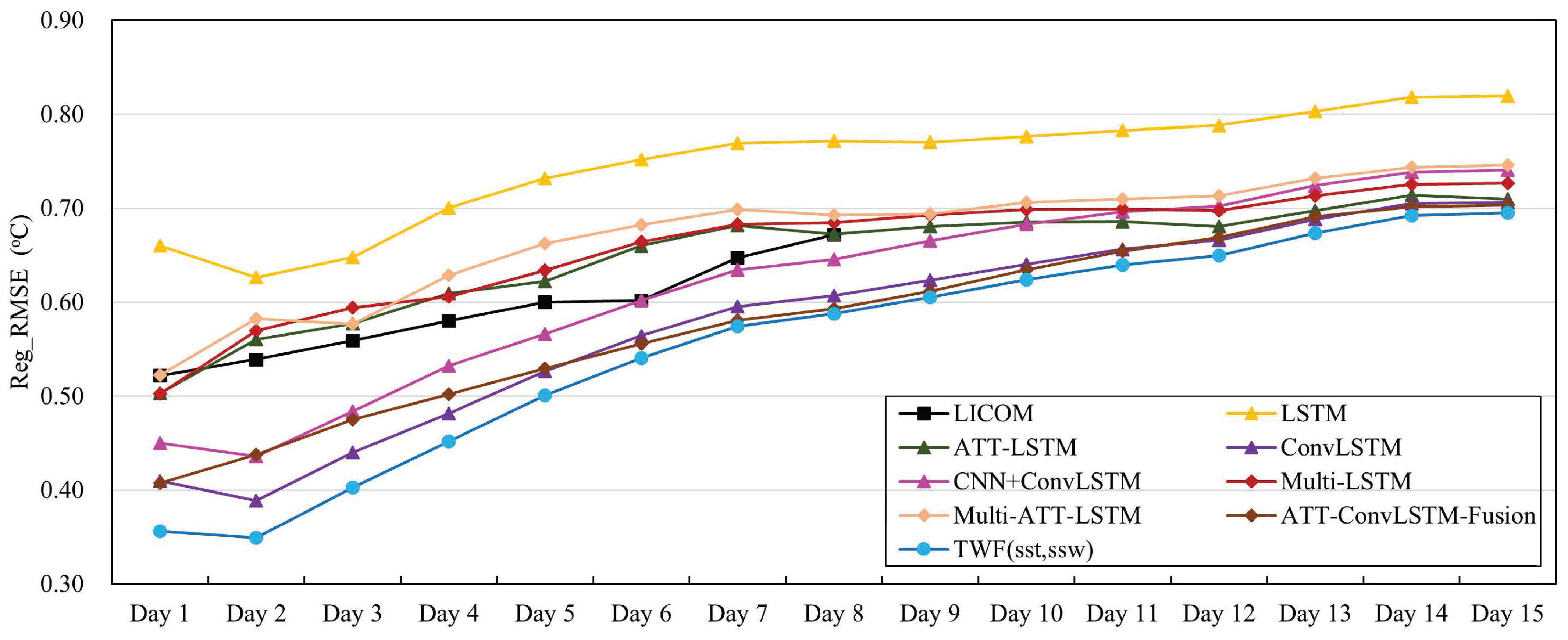
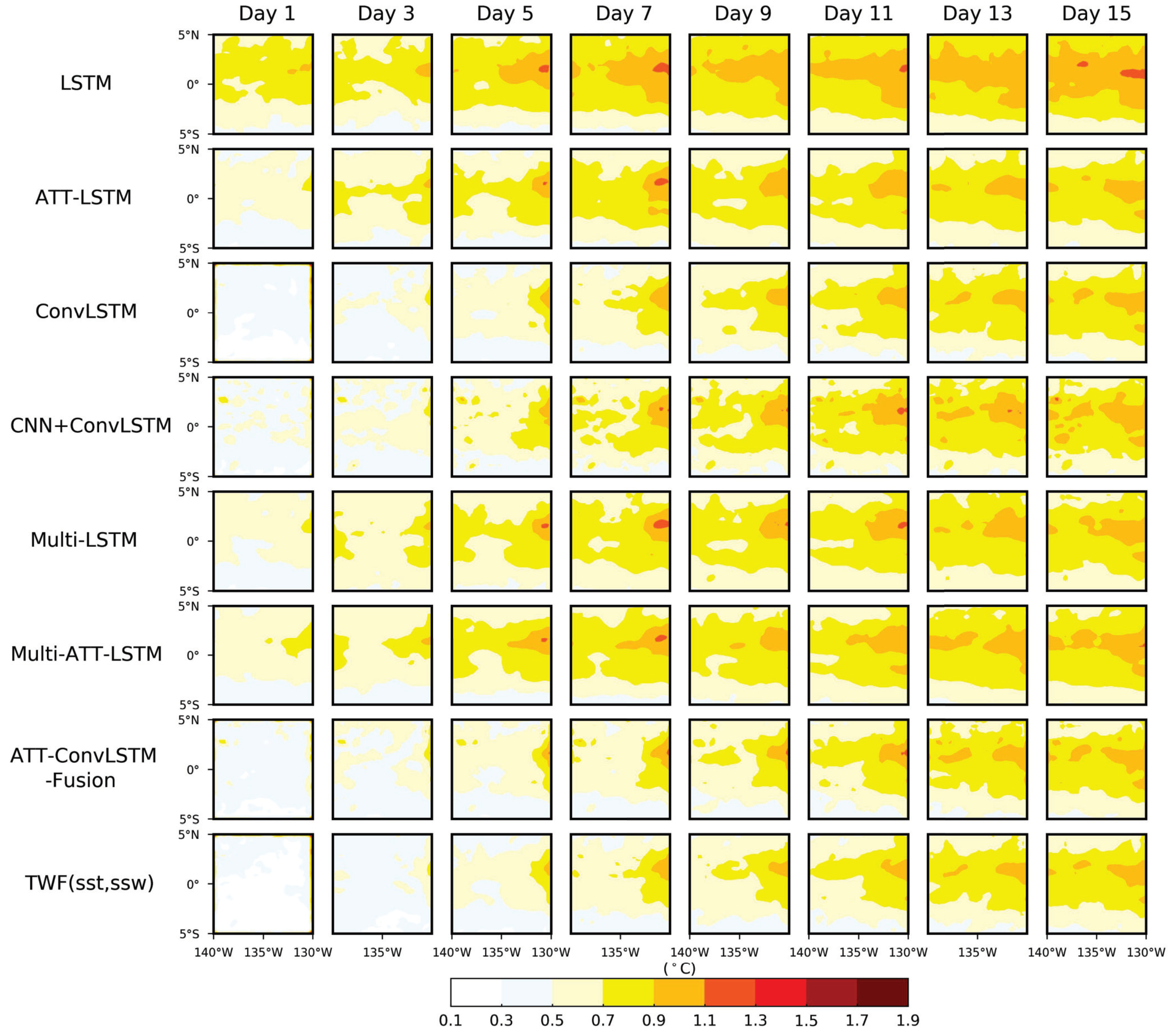
- The TWF(sst, ssw) model was compared with other benchmark models. The Poi_RMSE in the region with a latitude range of 0–5° N was larger than the Poi_RMSE in the region with a latitude range of 0–5° S among all the models. The TWF(sst, ssw) model had the smallest Reg_RMSE and the highest Reg_PACC on every day. Statistically, this indicates the superiority of the TWF(sst, ssw) model. Meanwhile, adding convolutions or ConvLSTM when building the model could effectively reduce the regional prediction error and improve the regional prediction accuracy.
- (3)
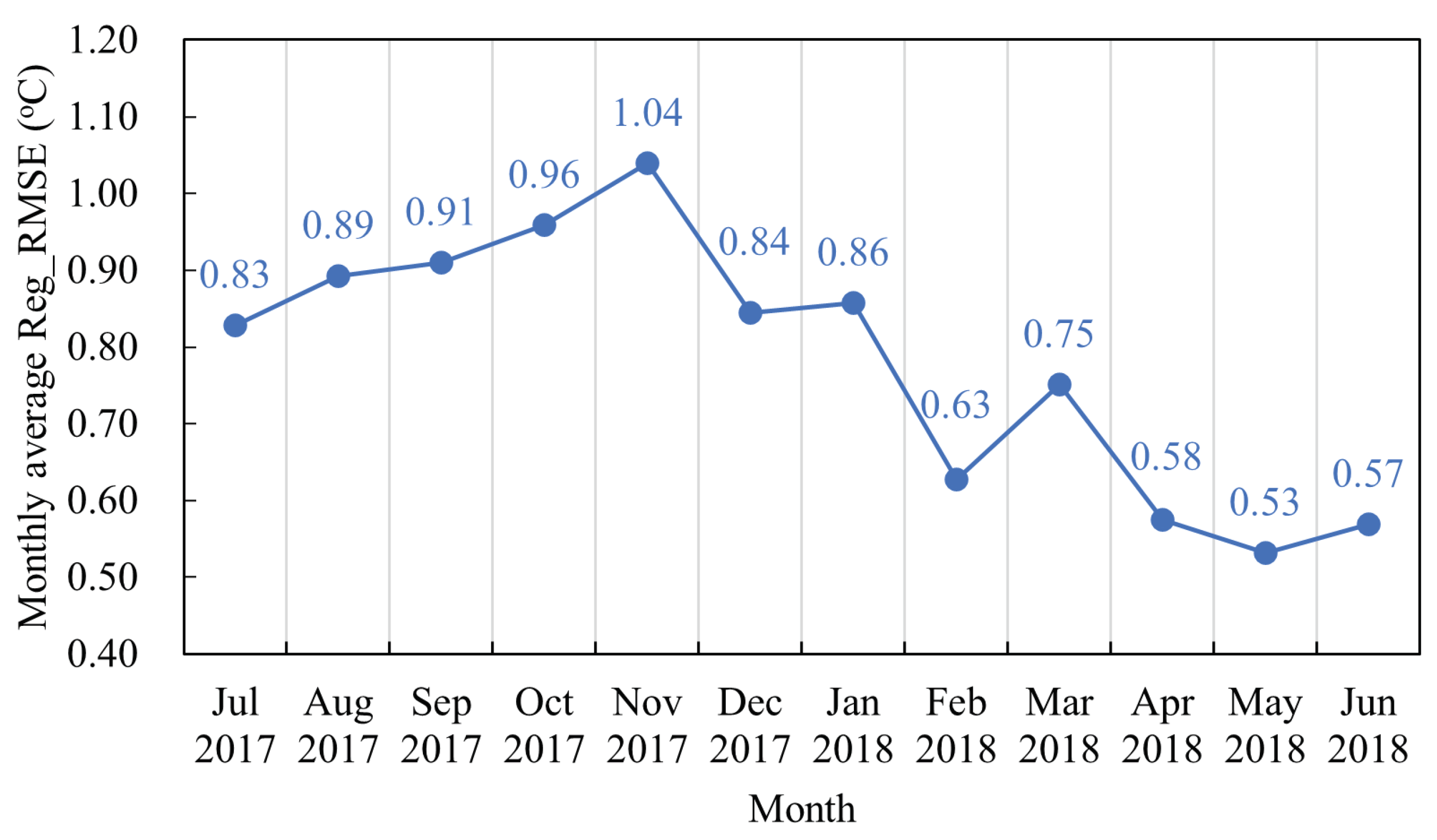
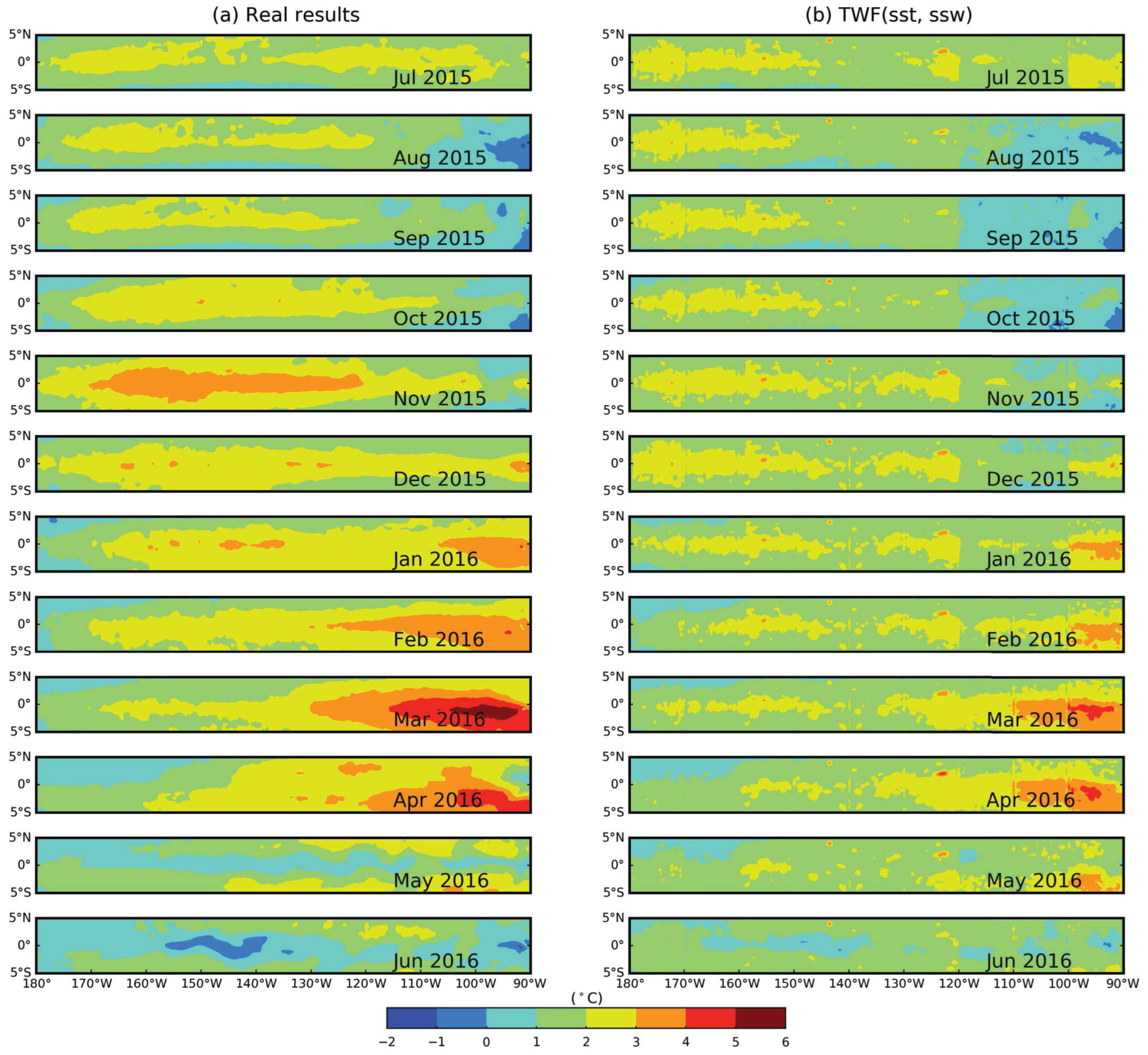
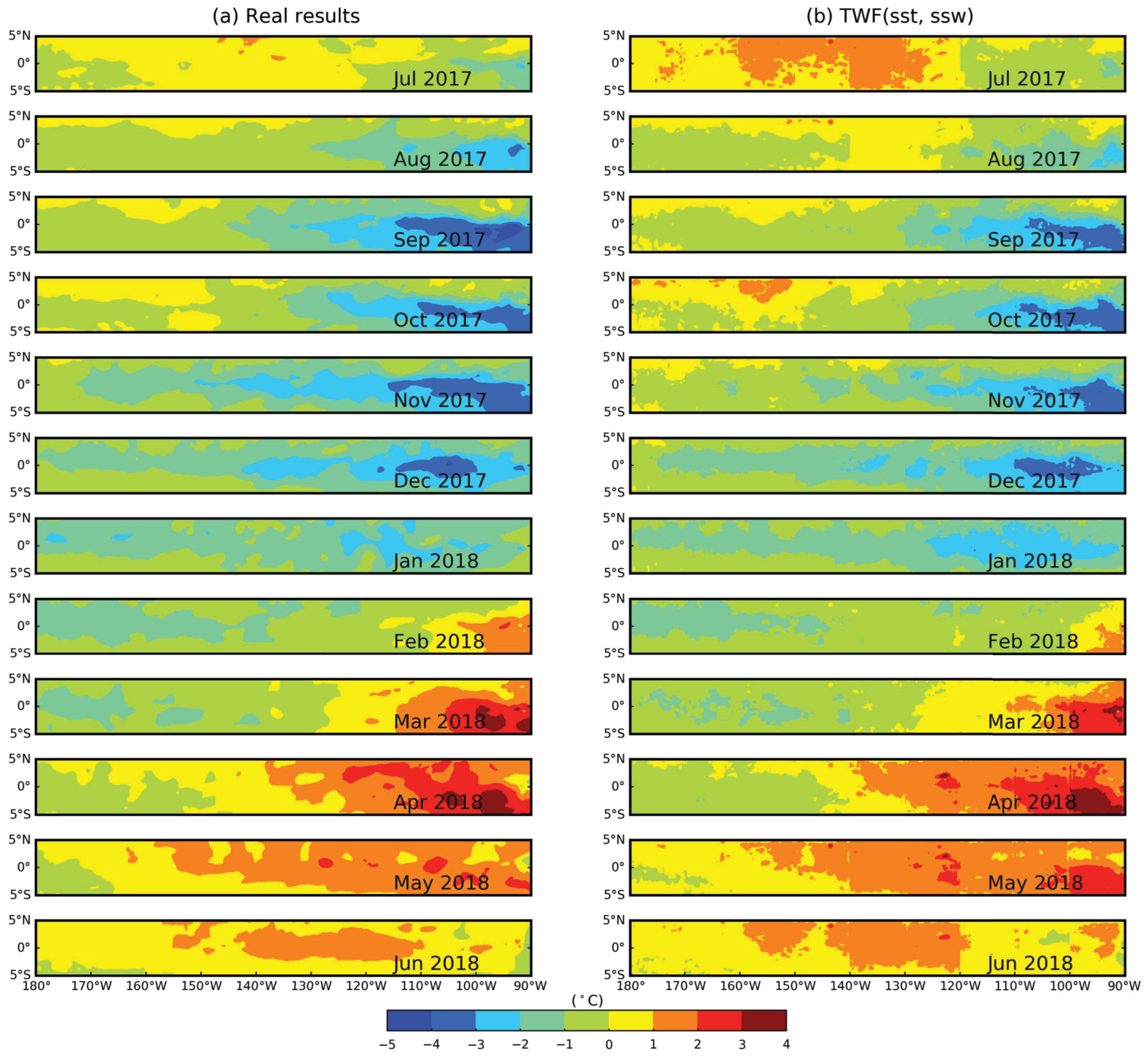
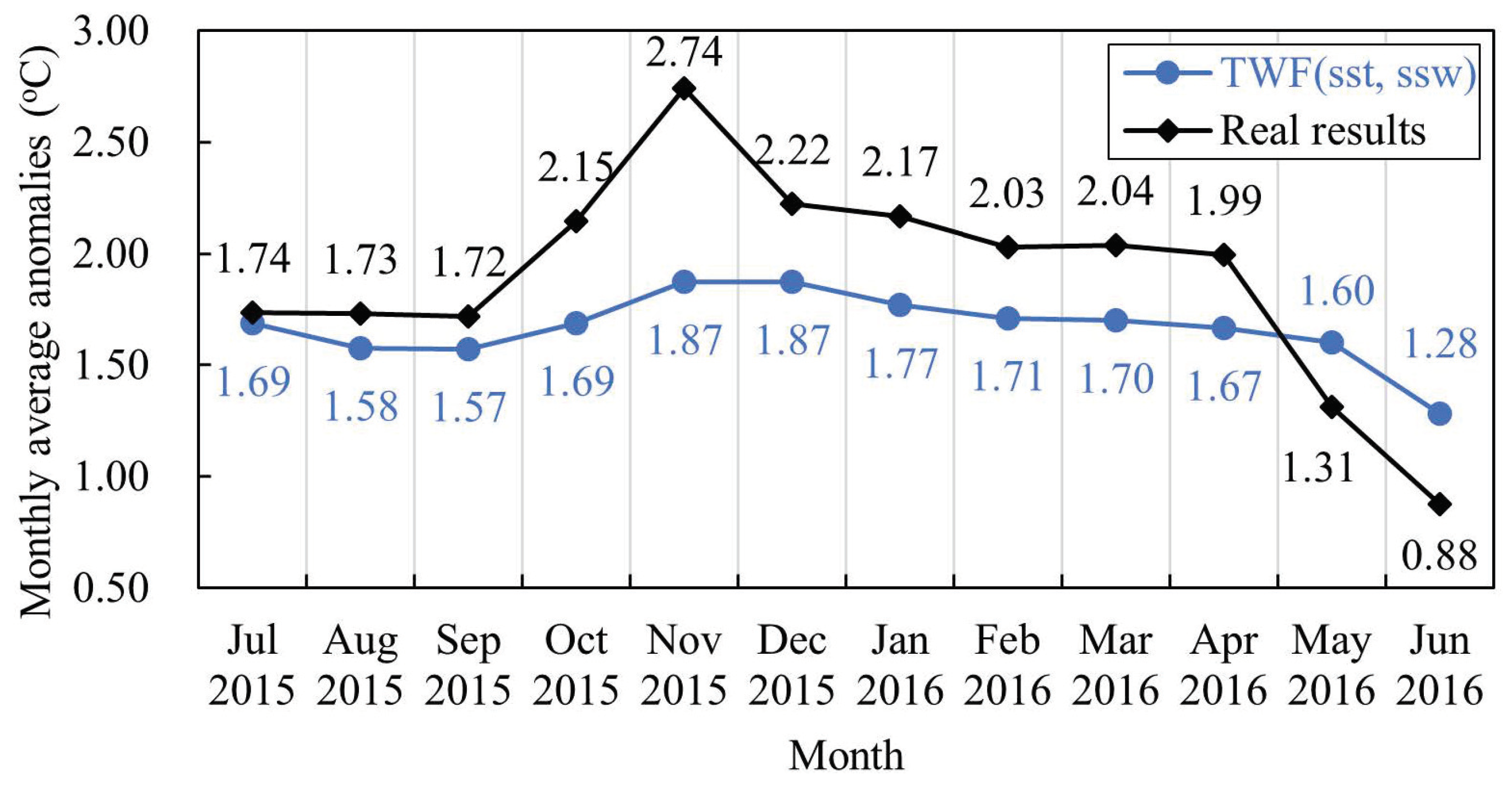
- In the equatorial Pacific during El Niño years, most of the prediction Bias values for the TWF(sst, ssw) model were less than 0.9 °C, and the monthly mean Poi_RMSE was less than 1.2 °C. In the equatorial Pacific during La Niña years, most of the prediction Bias values of the TWF (sst, ssw) model were less than 0.8 °C, and the monthly mean Poi_RMSE was less than 1.2 °C. The Poi_RMSE in El Niño and La Niña years was mainly concentrated in the range of 0.4–0.8 °C. The TWF(sst, ssw) model had better prediction performance in El Niño and La Niña years, but the prediction results of the model in La Niña years were better than those in El Niño years. This may have been related to the weak La Niña activity from 2017 to 2018 and the very strong El Niño activity from 2015 to 2016.
Author Contributions
Funding
Data Availability Statement
Conflicts of Interest
References
- Watanabe, M.; Dufresne, J.L.; Kosaka, Y.; Mauritsen, T.; Tatebe, H. Enhanced warming constrained by past trends in equatorial Pacific sea surface temperature gradient. Nat. Clim. Change 2021, 11, 33–37. [Google Scholar] [CrossRef]
- Bulgin, C.E.; Merchant, C.J.; Ferreira, D. Tendencies, variability and persistence of sea surface temperature anomalies. Sci. Rep. 2020, 10, 7986. [Google Scholar] [CrossRef]
- Seager, R.; Cane, M.; Henderson, N.; Lee, D.E.; Abernathey, R.; Zhang, H. Strengthening tropical Pacific zonal sea surface temperature gradient consistent with rising greenhouse gases. Nat. Clim. Change 2019, 9, 517–522. [Google Scholar] [CrossRef]
- Zhao, Y.; Sun, W.; Jie, Z. Analysis of SST Spatial and Temporal Characteristics in the North Pacific Using Remote Sensing Data. In Proceedings of the IGARSS 2022—2022 IEEE International Geoscience and Remote Sensing Symposium, Kuala Lumpur, Malaysia, 17–22 July 2022; pp. 6891–6894. [Google Scholar]
- Li, B.; Li, Y.; Chen, Y.; Zhang, B.; Shi, X. Recent fall Eurasian cooling linked to North Pacific sea surface temperatures and a strengthening Siberian high. Nat. Commun. 2020, 11, 5202. [Google Scholar] [CrossRef] [PubMed]
- Ferster, B.S.; Subrahmanyam, B.; Arguez, A. Recent Changes in Southern Ocean Circulation and Climate. IEEE Geosci. Remote Sens. Lett. 2019, 16, 667–671. [Google Scholar] [CrossRef]
- Ganguly, D.; Raman, M. Coastal Upwelling During Normal and EL Nino Years: Case Study of Peru and Oman Upwelling. In Proceedings of the 2021 IEEE International India Geoscience and Remote Sensing Symposium, Ahmedabad, India, 6–10 December 2021; pp. 107–110. [Google Scholar]
- Santillán, R.D.M.; Dongkai, Y.; Wang, H.; Zheng, L. Evidence of el niño-southem oscillation influence over the tropical glaciers in the santa river basin during the period 2001–2016. In Proceedings of the 2017 IEEE Region 10 Humanitarian Technology Conference, Dhaka, Bangladesh, 21–23 December 2017; pp. 34–37. [Google Scholar]
- Funk, C.; Harrison, L.; Shukla, S.; Pomposi, C.; Galu, G.; Korecha, D.; Husak, G.; Magadzire, T.; Davenport, F.; Korecha, D.; et al. Examining the role of unusually warm Indo-Pacific sea-surface temperatures in recent African droughts. Q. J. R. Meteorol. Soc. 2018, 144, 360–383. [Google Scholar] [CrossRef]
- Lachniet, M.S.; Asmerom, Y.; Polyak, V.; Denniston, R. Great Basin paleoclimate and aridity linked to Arctic warming and tropical Pacific sea surface temperatures. Paleoceanogr. Paleoclimatol. 2020, 35, e2019PA003785. [Google Scholar] [CrossRef]
- Cook, B.I.; Williams, A.P.; Smerdon, J.E.; Palmer, J.G.; Cook, E.R.; Stahle, D.W.; Coats, S. Cold tropical Pacific sea surface temperatures during the late sixteenth-century North American megadrought. J. Geophys. Res. Atmos. 2018, 123, 11307–11320. [Google Scholar] [CrossRef]
- Liu, Y.; Li, Z.; Yin, H. A timely El Niño-Southern Oscillation forecast method based on daily Niño index to ensure food security. In Proceedings of the 2018 7th International Conference on Agro-Geoinformatics, Hangzhou, China, 6–9 August 2018; pp. 1–6. [Google Scholar]
- Uzun, A.; Ustaoğlu, B. Impacts of El Nino Southern Oscillation (ENSO) and North Atlantic Oscillation (NAO) on the olive yield in the mediterranean region, Turkey. In Proceedings of the 2019 8th International Conference on Agro-Geoinformatics, Istanbul, Turkey, 16–19 July 2019; pp. 1–6. [Google Scholar]
- Hashemi, M. Forecasting El Nino and La Nina using spatially and temporally structured predictors and a convolutional neural network. IEEE J. Sel. Top. Appl. Earth Obs. Remote Sens. 2021, 14, 3438–3446. [Google Scholar] [CrossRef]
- Xing, D.; Zhang, W.; Huang, Q.; Liu, B. Research on Extreme Learning Machine Algorithm and Its Application to El-Niño/La-Niña Southern Oscillation Model. In Proceedings of the 2016 8th International Conference on Intelligent Human-Machine Systems and Cybernetics, Hangzhou, China, 27–28 August 2016; pp. 208–211. [Google Scholar]
- Barrientos, A.; Pino, E.; Uribe, C. Technological solutions for the detection and warning of natural disasters caused by the “El Niño” Phenomenon. In Proceedings of the 2019 IEEE XXVI International Conference on Electronics, Electrical Engineering and Computing, Lima, Peru, 12–14 August 2019; pp. 1–4. [Google Scholar]
- Hou, S.; Li, W.; Liu, T.; Zhou, S.; Guan, J.; Qin, R.; Wan, Z. MIMO: A Unified Spatio-Temporal Model for Multi-Scale Sea Surface Temperature Prediction. Remote Sens. 2022, 14, 2371. [Google Scholar] [CrossRef]
- Yokoyama, R.; Souma, T.; Tamba, S.; Konda, M. Sea surface effect on sea surface temperature detection by remote sensing. In Proceedings of the IGARSS’93—IEEE International Geoscience and Remote Sensing Symposium, Tokyo, Japan, 18–21 August 1993; pp. 140–142. [Google Scholar]
- Cui, Y.; Qiu, Y.; Sun, L.; Shu, X.; Lu, Z. Quantitative Short-Term Precipitation Model Using Multimodal Data Fusion Based on a Cross-Attention Mechanism. Remote Sens. 2022, 14, 5839. [Google Scholar] [CrossRef]
- Jia, X.; Ji, Q.; Han, L.; Liu, Y.; Han, G.; Lin, X. Prediction of Sea Surface Temperature in the East China Sea Based on LSTM Neural Network. Remote Sens. 2022, 14, 3300. [Google Scholar] [CrossRef]
- Ren, H.L.; Lu, B.; Wan, J.H.; Tian, B.; Zhang, P.Q. Identification standard of ENSO events and its application to climate monitoring and prediction in China. J. Meteor. Res. 2018, 32, 923–936. [Google Scholar] [CrossRef]
- Chen, D.; Zebiak, S.E.; Busalacchi, A.J.; Cane, M.A. An improved procedure for El Niño forecasting: Implications for predict ability. Science 1995, 269, 1699–1702. [Google Scholar] [CrossRef] [PubMed]
- Kirtman, P.B. The COLA anomaly coupled model: Ensem ble ENSO prediction. Mon. Weather Rev. 2003, 131, 2324–2341. [Google Scholar] [CrossRef]
- Ren, H.L.; Zuo, J.; Deng, Y. Statistical predictability of Niño indices for two types of ENSO. Clim. Dyn. 2019, 52, 5361–5382. [Google Scholar] [CrossRef]
- Zhang, Y.; Wang, R.; Yang, M.; Zhu, M.; Ye, C. Using full-traversal addition-subtraction frequency (ASF) method to predict possible el nino events in 2019, 2020 and so forth. In Proceedings of the 2018 Chinese Control And Decision Conference, Shenyang, China, 9–11 June 2018; pp. 2652–2657. [Google Scholar]
- Zhang, X.; Zhang, W.; Li, Y. Characteristics of the sea temperature in the North Yellow Sea. Mar. Forecasts 2015, 32, 89–97. [Google Scholar]
- Li, Z.; He, J.; Ni, T.; Huo, J. Numerical computation based few-shot learning for intelligent sea surface temperature prediction. Multimed. Syst. 2022, 29, 3001–3013. [Google Scholar] [CrossRef]
- Kug, J.S.; Kang, I.S.; Lee, J.Y.; Jhun, J.G. A statistical approach to Indian Ocean sea surface temperature prediction using a dynamical ENSO prediction. Geophys. Res. Lett. 2004, 31, L09212. [Google Scholar] [CrossRef]
- Zhao, Y.; Yang, D.; He, Z.; Liu, C.; Hao, R.; He, J. Statistical Methods in Ocean Prediction. In Proceedings of the Global Oceans 2020: Singapore–US Gulf Coast, Biloxi, MS, USA, 5–30 October 2020; pp. 1–7. [Google Scholar]
- Wu, A.; Hsieh, W.W.; Tang, B. Neural network forecasts of the tropical Pacific sea surface temperatures. Neural Netw. 2006, 19, 145–154. [Google Scholar] [CrossRef]
- Ji, J.; Zhang, L. Prediction of sea surface temperature by Kalman filtering. Mar. Forecasts 2010, 27, 59–65. [Google Scholar]
- Wei, L.; Guan, L.; Qu, L.; Guo, D. Prediction of Sea Surface Temperature in the China Seas Based on Long Short-Term Memory Neural Networks. Remote Sens. 2020, 12, 2697. [Google Scholar] [CrossRef]
- Han, M.; Feng, Y.; Zhao, X.; Sun, C.; Hong, F.; Liu, C. A convolutional neural network using surface data to predict subsurface temperatures in the Pacific Ocean. IEEE Access 2019, 7, 172816–172829. [Google Scholar] [CrossRef]
- Kalchbrenner, N.; Oord, A.; Simonyan, K.; Danihelka, I.; Vinyals, O.; Graves, A.; Kavukcuoglu, K. Video pixel networks. arXiv 2016, arXiv:1610.00527. [Google Scholar]
- Wang, Y.; Long, M.; Wang, J.; Gao, Z.; Yu, P.S. PredRNN: Recurrent neural networks for predictive learning using spatiotemporal LSTMs. Adv. Neural Inf. Process. Syst. 2017, 30, 879–888. [Google Scholar]
- Wang, Y.; Gao, Z.; Long, M.; Wang, J.; Philip, S.Y. Predrnn++: Towards a resolution of the deep-in-time dilemma in spatiotemporal predictive learning. arXiv 2018, arXiv:1804.06300. [Google Scholar]
- Liu, J.; Zhang, T.; Gou, Y.; Wang, X.; Li, B.; Guan, W. Convolutional LSTM networks for seawater temperature prediction. In Proceedings of the 2019 IEEE International Conference on Signal, Information and Data Processing, Chongqing, China, 11–13 December 2019; pp. 1–5. [Google Scholar]
- Xu, L.; Li, Q.; Yu, J.; Wang, L.; Xie, J.; Shi, S. Spatio-temporal predictions of SST time series in China’s offshore waters using a regional convolution long short-term memory (RC-LSTM) network. Int. J. Remote Sens. 2020, 41, 3368–3389. [Google Scholar] [CrossRef]
- Gou, Y.; Zhang, T.; Liu, J.; Wei, L.; Cui, J.H. DeepOcean: A general deep learning framework for spatio-temporal ocean sensing data prediction. IEEE Access 2020, 8, 79192–79202. [Google Scholar] [CrossRef]
- Wang, G.; Wang, X.; Wu, X.; Liu, K.; Qi, Y.; Sun, C.; Fu, H. Multimodal fusion for sea level anomaly forecasting. arXiv 2020, arXiv:2006.08209. [Google Scholar]
- Hou, S.; Li, W.; Liu, T.; Zhou, S.; Guan, J.; Qin, R.; Wang, Z. Must: A multi-source spatio-temporal data fusion model for short-term sea surface temperature prediction. Ocean Eng. 2022, 259, 111932. [Google Scholar] [CrossRef]
- Lin, Z.; Li, M.; Zheng, Z.; Cheng, Y.; Yuan, C. Self-attention convlstm for spatiotemporal prediction. In Proceedings of the AAAI Conference on Artificial Intelligence, New York, NY, USA, 7–12 February 2020; AAAI Press: Palo Alto, CA, USA, 2020; pp. 11531–11538. [Google Scholar]
- Li, B.; Tang, B.; Deng, L.; Zhao, M. Self-attention ConvLSTM and its application in RUL prediction of rolling bearings. IEEE Trans. Instrum. Meas. 2021, 70, 3518811. [Google Scholar] [CrossRef]
- Zhou, Y.; Huo, C.; Zhu, J.; Huo, L.; Pan, C. DCAT: Dual Cross-Attention-Based Transformer for Change Detection. Remote Sens. 2023, 15, 2395. [Google Scholar] [CrossRef]
- Zhou, L.; Zhang, R.H. A self-attention–based neural network for three-dimensional multivariate modeling and its skillful ENSO predictions. Sci. Adv. 2023, 9, eadf2827. [Google Scholar] [CrossRef]
- Schneider, D.P.; Deser, C.; Fasullo, J.; Trenberth, K.E. Climate Data Guide Spurs Discovery and Understanding. Eos Trans. AGU 2013, 94, 121–122. [Google Scholar] [CrossRef]
- Boy, F.; Picot, N.; Desjonqueres, J.D. CryoSat Processing Prototype, LRM Processing on CNES Side and a Comparison to DUACS SLA. Geophys. Res. Abstr. 2011, 13, 8323. [Google Scholar]
- Saha, K.; Zhang, H.M. Hurricane and Typhoon Storm Wind Resolving NOAA NCEI Blended Sea Surface Wind (NBS) Product. Front. Mar. Sci. 2022, 9, 935549. [Google Scholar] [CrossRef]
- Wang, S.; Yu, J.; Meng, J. Echo State Network based on Phase Space Reconstruction: El Niño 3 Index Forecasting. In Proceedings of the 2020 Chinese Control and Decision Conference, Hefei, China, 22–24 August 2020; pp. 29–33. [Google Scholar]
- Santillán, R.D.M.; Dongkai, Y.; Wang, H.; Zheng, L. Snow cover variation in santa river basin and its relation to sea surface temperature anomaly in the pacific ocean during the period 2003–2016. In Proceedings of the 2017 IEEE Region 10 Humanitarian Technology Conference, Dhaka, Bangladesh, 21–23 December 2017; pp. 93–96. [Google Scholar]
- Putra, I.D.G.A.; Heriyanto, E.; Sopaheluwakan, A.; Pradana, R.P.; Nuryanto, D.E. Seasonal Analysis of the Hotspot Spatial Grid in Indonesia and the Relationship of the Hotspot Grid with the Nino SST Indices. In Proceedings of the 2020 IEEE Asia-Pacific Conference on Geoscience, Electronics and Remote Sensing Technology, Jakarta, Indonesia, 7–8 December 2020; pp. 63–68. [Google Scholar]
- Shi, X.; Chen, Z.; Wang, H.; Yeung, D.Y.; Wong, W.K.; Woo, W.C. Convolutional LSTM network: A machine learning approach for precipitation nowcasting. In Proceedings of the 29th International Conference on Neural Information Processing Systems, Montreal, QC, Canada, 7–12 December 2015; pp. 802–810. [Google Scholar]
- Hu, W.S.; Li, H.C.; Pan, L.; Li, W.; Tao, R.; Du, Q. Spatial–spectral feature extraction via deep ConvLSTM neural networks for hyperspectral image classification. IEEE Trans. Geosci. Remote Sens. 2020, 58, 4237–4250. [Google Scholar] [CrossRef]
- Wang, L.; Shen, L. A ConvLSTM-combined hierarchical attention network for saliency detection. In Proceedings of the 2020 IEEE International Conference on Image Processing, Abu Dhabi, United Arab Emirates, 25–28 October 2020; pp. 1996–2000. [Google Scholar]
- Liu, H.; Lin, P.; Zheng, W.; Luan, Y.; Ma, J.; Ding, M.; Mo, H.; Wan, L.; Ling, T. A global eddy-resolving ocean forecast system in China-LICOM Forecast System (LFS). J. Oper. Oceanog. 2023, 16, 15–27. [Google Scholar] [CrossRef]
- Geng, X.; Zhang, W.J.; Stuecker, M.F.; Jin, F.F. Strong sub-seasonal wintertime cooling over East Asia and Northern Europe associated with super El Niño events. Sci. Rep. 2017, 7, 3770. [Google Scholar] [CrossRef]
- Rädel, G.; Mauritsen, T.; Stevens, B.; Dommenget, D.; Matei, D.; Bellomo, K.; Clement, C. Amplification of El Niño by cloud longwave coupling to atmospheric circulation. Nat. Geosci. 2016, 9, 106–110. [Google Scholar] [CrossRef]
- Serykh, I.; Sonechkin, D. El Niño–Global Atmospheric Oscillation as the Main Mode of Interannual Climate Variability. Atmosphere 2021, 12, 1443. [Google Scholar] [CrossRef]
- Zhan, P.M.; Yu, R.; Guo, Y.J.; Li, Q.X.; Ren, X.J.; Wang, Y.Q.; Xu, W.H.; Liu, Y.J.; Ding, Y.H. The strong El Niño in 2015/2016 and its dominant impacts on global and China’s climate. Acta. Meteorol. Sin. 2016, 74, 309–321. [Google Scholar]


| Statistics | SST | SLA | SSW |
|---|---|---|---|
| Total grid points | 14,400 | 14,400 | 14,400 |
| Invalid grid points (Nan) | 2 | 3 | 21 |
| Valid grid points | 14,398 | 14,397 | 14,379 |
| Module Units | Functional Description | Parameter Setting |
|---|---|---|
| Conv3D | Extracting temporal feature timing information | filters = 40, kernel_size = (3, 3, 3) |
| Conv3D_A | Extracting temporal feature timing information | filters = 1, kernel_size = (1, 1, 1) |
| Add | Fuse features of multiple elements so only the amount of information increases, without changing the dimensionality of the image | - |
| Activation | Perform processing of nonlinear mapping | ‘relu’ or ‘sigmoid’ |
| Transpose | Swap different dimensions of the input tensor | perm = [0, 4, 2, 3, 1] |
| Multiply | Compute the product (element by element) of the input tensor list | - |
| ConvLSTM2D | Capture long time series dependencies, memorize and store information | filters = 32, kernel_size = (3, 3, 3), recurrent_dropout = 0.2 |
| Conversion | Convert the input shape (timesteps, rows, cols) to (targetsizes, rows, cols) | target size = targetsizes |
| Dense | Mapping the extracted features to the output through a nonlinear transformation | units = 1 |
| Parameters | Day 1 | 5-Day Average | 10-Day Average | 15-Day Average | |||||
|---|---|---|---|---|---|---|---|---|---|
| targetsizes | timesteps | Reg_RMSE | Reg_PACC | Reg_RMSE | Reg_PACC | Reg_RMSE | Reg_PACC | Reg_RMSE | Reg_PACC |
| 5 | 5 | 0.5933 | 0.9793 | 0.6419 | 0.9780 | - | - | - | - |
| 10 | 0.4018 | 0.9876 | 0.4793 | 0.9847 | - | - | - | - | |
| 15 | 0.4341 | 0.9860 | 0.5322 | 0.9827 | - | - | - | - | |
| 20 | 0.5271 | 0.9844 | 0.5437 | 0.9827 | - | - | - | - | |
| 10 | 10 | 0.5460 | 0.9827 | 0.5620 | 0.9818 | 0.6581 | 0.9782 | - | - |
| 15 | 0.5104 | 0.9841 | 0.5387 | 0.9827 | 0.6305 | 0.9793 | - | - | |
| 20 | 0.4248 | 0.9874 | 0.4608 | 0.9854 | 0.5547 | 0.9818 | - | - | |
| 30 | 0.5028 | 0.9842 | 0.5335 | 0.9831 | 0.6179 | 0.9800 | - | - | |
| 40 | 0.4418 | 0.9861 | 0.5242 | 0.9831 | 0.6286 | 0.9793 | - | - | |
| 15 | 15 | 0.5410 | 0.9832 | 0.5480 | 0.9824 | 0.6288 | 0.9793 | 0.6672 | 0.9779 |
| 20 | 0.5620 | 0.9824 | 0.5914 | 0.9806 | 0.6782 | 0.9772 | 0.7231 | 0.9755 | |
| 30 | 0.4564 | 0.9865 | 0.4673 | 0.9854 | 0.5403 | 0.9828 | 0.5752 | 0.9816 | |
| 40 | 0.8976 | 0.9692 | 0.8452 | 0.9712 | 0.8036 | 0.9730 | 0.7769 | 0.9739 | |
| Indicators | Models | Day 1 | Day 3 | Day 5 | Day 7 | Day 9 | Day 11 | Day 13 | Day 15 | Ave-Day |
|---|---|---|---|---|---|---|---|---|---|---|
| Reg_RMSE | TF(sst) | 0.5425 | 0.6359 | 0.8958 | 0.8509 | 0.9445 | 0.9868 | 0.9833 | 0.7932 | 0.8432 |
| TAF(sst, sla) | 0.2274 | 0.3126 | 0.5501 | 0.5289 | 0.5941 | 0.6452 | 0.6474 | 0.5180 | 0.5132 | |
| TWF(sst, ssw) | 0.2959 | 0.3066 | 0.4267 | 0.4038 | 0.4460 | 0.5148 | 0.5488 | 0.5129 | 0.4316 | |
| TAWF(sst,sla,ssw) | 0.2576 | 0.4225 | 0.7193 | 0.7039 | 0.8002 | 0.8425 | 0.8436 | 0.6736 | 0.6746 | |
| Reg_PACC | TF(sst) | 0.9802 | 0.9776 | 0.9687 | 0.9706 | 0.9664 | 0.9657 | 0.9673 | 0.9746 | 0.9708 |
| TAF(sst, sla) | 0.9937 | 0.9901 | 0.9828 | 0.9829 | 0.9804 | 0.9788 | 0.9796 | 0.9842 | 0.9836 | |
| TWF(sst, ssw) | 0.9913 | 0.9905 | 0.9870 | 0.9873 | 0.9863 | 0.9840 | 0.9832 | 0.9847 | 0.9868 | |
| TAWF(sst,sla,ssw) | 0.9924 | 0.9861 | 0.9755 | 0.9757 | 0.9713 | 0.9706 | 0.9719 | 0.9786 | 0.9771 |
| Models | Location A | Location B | Location C | Location D | ||||
|---|---|---|---|---|---|---|---|---|
| Poi_RMSE | Poi_PACC | Poi_RMSE | Poi_PACC | Poi_RMSE | Poi_PACC | Poi_RMSE | Poi_PACC | |
| TF(sst) | 0.5717 | 0.9829 | 0.8618 | 0.9746 | 0.3725 | 0.9887 | 0.3908 | 0.9880 |
| TAF(sst, sla) | 0.3570 | 0.9903 | 0.7760 | 0.9760 | 0.3252 | 0.9904 | 0.3030 | 0.9913 |
| TWF(sst, ssw) | 0.3764 | 0.9896 | 0.7448 | 0.9776 | 0.3019 | 0.9911 | 0.2732 | 0.9921 |
| TAWF(sst,sla,ssw) | 0.4316 | 0.9878 | 0.7769 | 0.9765 | 0.3572 | 0.9891 | 0.3377 | 0.9895 |
| Indicators | Models | Day 1 | Day 3 | Day 5 | Day 7 | Day 9 | Day 11 | Day 13 | Day 15 | Ave-Day |
|---|---|---|---|---|---|---|---|---|---|---|
| Reg_RMSE | LICOM | 0.5220 | 0.5590 | 0.6000 | 0.6470 | - | - | - | - | 0.5901 |
| LSTM | 0.6602 | 0.6479 | 0.7320 | 0.7694 | 0.7703 | 0.7824 | 0.8033 | 0.8193 | 0.7478 | |
| ATT-LSTM | 0.5034 | 0.5774 | 0.6222 | 0.6817 | 0.6804 | 0.6857 | 0.6977 | 0.7099 | 0.6493 | |
| ConvLSTM | 0.4095 | 0.4401 | 0.5263 | 0.5955 | 0.6234 | 0.6563 | 0.6880 | 0.7062 | 0.5798 | |
| CNN+ConvLSTM | 0.4501 | 0.4841 | 0.5663 | 0.6342 | 0.6652 | 0.6963 | 0.7240 | 0.7406 | 0.6200 | |
| Multi-LSTM | 0.5024 | 0.5941 | 0.6340 | 0.6831 | 0.6928 | 0.6992 | 0.7131 | 0.7264 | 0.6594 | |
| Multi-ATT-LSTM | 0.5225 | 0.5769 | 0.6626 | 0.6985 | 0.6941 | 0.7095 | 0.7320 | 0.7458 | 0.6727 | |
| ATT-ConvLSTM-Fusion | 0.4072 | 0.4752 | 0.5294 | 0.5805 | 0.6118 | 0.6540 | 0.6909 | 0.7033 | 0.5831 | |
| TWF(sst, ssw) | 0.3563 | 0.4026 | 0.5005 | 0.5742 | 0.6052 | 0.6395 | 0.6735 | 0.6950 | 0.5561 | |
| Reg_PACC | LSTM | 0.9782 | 0.9794 | 0.9765 | 0.9752 | 0.9751 | 0.9748 | 0.9740 | 0.9735 | 0.9759 |
| ATT-LSTM | 0.9843 | 0.9817 | 0.9805 | 0.9782 | 0.9783 | 0.9783 | 0.9778 | 0.9773 | 0.9794 | |
| ConvLSTM | 0.9883 | 0.9867 | 0.9840 | 0.9817 | 0.9808 | 0.9797 | 0.9785 | 0.9778 | 0.9822 | |
| CNN+ConvLSTM | 0.9854 | 0.9847 | 0.9822 | 0.9799 | 0.9792 | 0.9781 | 0.9772 | 0.9765 | 0.9804 | |
| Multi-LSTM | 0.9845 | 0.9809 | 0.9798 | 0.9780 | 0.9778 | 0.9777 | 0.9771 | 0.9766 | 0.9789 | |
| Multi-ATT-LSTM | 0.9836 | 0.9819 | 0.9791 | 0.9778 | 0.9779 | 0.9775 | 0.9766 | 0.9762 | 0.9787 | |
| ATT-ConvLSTM-Fusion | 0.9876 | 0.9854 | 0.9838 | 0.9821 | 0.9812 | 0.9797 | 0.9784 | 0.9779 | 0.9820 | |
| TWF(sst, ssw) | 0.9901 | 0.9879 | 0.9848 | 0.9823 | 0.9813 | 0.9802 | 0.9789 | 0.9781 | 0.9829 |
| Jul. 2015 | Aug. 2015 | Sep. 2015 | Oct. 2015 | Nov. 2015 | Dec. 2015 | Jan. 2016 | Feb. 2016 | Mar. 2016 | Apr. 2016 | May 2016 | Jun. 2016 | |
|---|---|---|---|---|---|---|---|---|---|---|---|---|
| 30.38% | 38.72% | 36.15% | 17.07% | 16.15% | 23.53% | 12.13% | 19.13% | 16.94% | 8.98% | 13.91% | 8.91% | |
| 61.31% | 50.36% | 47.99% | 53.28% | 38.33% | 56.18% | 51.84% | 48.76% | 42.07% | 35.24% | 43.85% | 41.92% | |
| 7.33% | 8.05% | 13.47% | 26.02% | 29.56% | 18.05% | 29.77% | 21.81% | 21.53% | 36.28% | 22.31% | 28.16% | |
| 0.94% | 1.79% | 1.92% | 3.51% | 14.26% | 2.19% | 5.83% | 8.69% | 15.58% | 17.92% | 15.40% | 13.30% | |
| 0.05% | 0.72% | 0.42% | 0.11% | 1.71% | 0.06% | 0.40% | 1.60% | 3.64% | 1.29% | 3.89% | 4.51% | |
| - | 0.36% | 0.03% | - | - | - | 0.03% | 0.01% | 0.24% | 0.29% | 0.63% | 3.19% |
| Jul. 2017 | Aug. 2017 | Sep. 2017 | Oct. 2017 | Nov. 2017 | Dec. 2017 | Jan. 2018 | Feb. 2018 | Mar. 2018 | Apr. 2018 | May 2018 | Jun. 2018 | |
|---|---|---|---|---|---|---|---|---|---|---|---|---|
| 10.28% | 21.31% | 10.78% | 8.57% | 6.16% | 8.77% | 5.93% | 23.78% | 24.49% | 28.24% | 36.28% | 38.92% | |
| 41.99% | 36.11% | 47.35% | 41.49% | 36.38% | 50.96% | 50.05% | 61.22% | 46.92% | 63.26% | 54.65% | 50.47% | |
| 39.24% | 23.94% | 23.50% | 30.31% | 28.45% | 28.22% | 32.28% | 10.58% | 18.40% | 6.56% | 8.22% | 7.40% | |
| 7.65% | 13.69% | 12.17% | 14.56% | 19.23% | 9.74% | 9.41% | 3.86% | 6.97% | 1.20% | 0.66% | 2.56% | |
| 0.77% | 3.95% | 5.56% | 3.89% | 7.95% | 1.99% | 1.95% | 0.47% | 2.36% | 0.48% | 0.11% | 0.64% | |
| 0.08% | 1.00% | 0.63% | 1.18% | 1.83% | 0.32% | 0.38% | 0.08% | 0.86% | 0.27% | 0.08% | 0.01% |
Disclaimer/Publisher’s Note: The statements, opinions and data contained in all publications are solely those of the individual author(s) and contributor(s) and not of MDPI and/or the editor(s). MDPI and/or the editor(s) disclaim responsibility for any injury to people or property resulting from any ideas, methods, instructions or products referred to in the content. |
© 2025 by the authors. Licensee MDPI, Basel, Switzerland. This article is an open access article distributed under the terms and conditions of the Creative Commons Attribution (CC BY) license (https://creativecommons.org/licenses/by/4.0/).
Share and Cite
Xu, T.; Zhou, Z.; Wang, C.; Li, Y.; Rong, T. Spatio-Temporal Prediction of Surface Remote Sensing Data in Equatorial Pacific Ocean Based on Multi-Element Fusion Network. J. Mar. Sci. Eng. 2025, 13, 755. https://doi.org/10.3390/jmse13040755
Xu T, Zhou Z, Wang C, Li Y, Rong T. Spatio-Temporal Prediction of Surface Remote Sensing Data in Equatorial Pacific Ocean Based on Multi-Element Fusion Network. Journal of Marine Science and Engineering. 2025; 13(4):755. https://doi.org/10.3390/jmse13040755
Chicago/Turabian StyleXu, Tianliang, Zhiquan Zhou, Chenxu Wang, Yingchun Li, and Tian Rong. 2025. "Spatio-Temporal Prediction of Surface Remote Sensing Data in Equatorial Pacific Ocean Based on Multi-Element Fusion Network" Journal of Marine Science and Engineering 13, no. 4: 755. https://doi.org/10.3390/jmse13040755
APA StyleXu, T., Zhou, Z., Wang, C., Li, Y., & Rong, T. (2025). Spatio-Temporal Prediction of Surface Remote Sensing Data in Equatorial Pacific Ocean Based on Multi-Element Fusion Network. Journal of Marine Science and Engineering, 13(4), 755. https://doi.org/10.3390/jmse13040755