Marine Multi-Physics-Based Hierarchical Fusion Recognition Method for Underwater Targets

Abstract

With the rapid advancement of ocean monitoring technology, the types and quantities of underwater sensors have increased significantly. Traditional single-sensor approaches exhibit limitations in underwater target classification, resulting in low classification accuracy and poor robustness. This paper integrates deep learning and information fusion theory to propose a multi-level fusion perception method for underwater targets based on multi-physical-field sensing. We extract both conventional typical features and deep features derived from an autoencoder and perform feature-level fusion. Neural network-based classification models are constructed for each physical field subsystem. To address the class imbalance and difficulty imbalance issues in the collected physical field target samples, we design a C-Focal Loss function specifically for the three underwater target categories. Furthermore, based on the confusion matrix results from the subsystem’s validation set, we propose a neural network-based Dempster–Shafer evidence fusion method (NNDS). Experimental validation using real-world data demonstrates a 97.15% fusion classification accuracy, significantly outperforming both direct multi-physical-field network fusion and direct subsystem decision fusion. The proposed method also exhibits superior reliability and robustness.

1. Introduction

Underwater target recognition technology has evolved alongside advancements in sonar technology, signal detection theory, and computer technology [1,2]. Subsequent progress in information theory, adaptive signal processing, and modern spectral estimation has driven further developments in this field. This technology holds significant importance across multiple domains [3]. In marine resource exploration, it enables the effective identification of underwater mineral deposits and biological resources to optimize resource utilization efficiency [4]. For military defense applications, underwater target recognition is critical for detecting and classifying submarines, unmanned underwater vehicles (UUVs), and other strategic threats, thereby enhancing national maritime defense capabilities [5]. In environmental conservation, the technology facilitates the monitoring of marine ecosystems and supports the timely identification and mitigation of environmental pollution issues [6].

Underwater target signals across various physical fields are inherently unstable due to the complex marine environment. These signals exhibit dynamic time–space–frequency variations, nonlinear and non-Gaussian characteristics, multipath effects, and interference from reverberation and environmental noise. A single sensor can only capture partial target information, leading to uncertainties in data acquisition and resulting in imprecise, incomplete, and unreliable observations [7]. Consequently, underwater target identification based solely on a single sensor suffers from low recognition accuracy, poor robustness, and limited reliability. To achieve a comprehensive and accurate perception of underwater targets, multi-sensor information fusion is essential.

Information fusion theory originated in underwater signal processing, and the marine domain has remained a primary area of focus for fusion research. In military applications, maritime information fusion serves as a core enabling technology for naval intelligence systems. In civilian applications, the demand for oceanic information fusion continues to grow in areas such as maritime safety monitoring, emergency response to maritime incidents, search and rescue operations, marine environmental protection, resource exploration, and disaster prevention [8,9]. Traditional methods in underwater target fusion perception include Fisher discriminant analysis, principal component analysis, rough set theory, approximate grid filtering, wavelet hierarchical image fusion, particle filtering, hidden Markov models, double Markov chain models, entropy-based approaches, and joint sparsity models (JSMs).

Several studies have contributed to the development of underwater target fusion recognition. J. Yong employed a voting-based fusion approach incorporating Dempster–Shafer (D-S) theory for local decision fusion, demonstrating enhanced robustness in low signal-to-noise-ratio (SNR) and adversarial environments [10]. J. Xu explored feature-level fusion of ship acoustic and magnetic field characteristics, utilizing correlation-based processing and M-S diagrams and achieving over 80% classification accuracy in sea trials [11]. X. Pan introduced an adaptive, multi-feature fusion network for underwater target recognition, incorporating data preprocessing, multi-dimensional feature extraction, and adaptive feature fusion modules to improve classification accuracy [12].

With the increasing demand for intelligent and rapid underwater target perception, research has shifted towards machine learning-based approaches. Neural network-based sensor information fusion offers a unified internal knowledge representation, enabling automatic knowledge acquisition and parallel associative reasoning. This has emerged as a key research focus in recent years [13]. X. Han proposed a one-dimensional convolutional neural network (1D-CNN) combined with a long short-term memory (LSTM) network, effectively leveraging the temporal characteristics of ship noise signals to enhance classification accuracy [14]. Q. Zhang developed a 2D-CNN-based approach to underwater target signal recognition, utilizing frequency-domain information. The proposed ensemble network, consisting of three distinct 2D-CNNs trained on different spectral representations, demonstrated improved recognition performance [15]. S. Zhang introduced both a feature-level fusion model based on multi-category feature subsets and a decision-level fusion model using D-S evidence theory, achieving superior classification performance compared to single-feature methods [16].

Deep learning-based methods have also been applied to underwater target perception. X. Cao designed a stacked sparse autoencoder (SSAE) model trained on a dataset comprising underwater acoustic signals from different ocean depths, achieving a 5% improvement in classification accuracy with joint feature inputs [17]. Y. Dong examined networked underwater target detection scenarios, demonstrating the efficiency of information fusion through case studies [18]. T. Fei integrated an ensemble learning scheme within the Dempster–Shafer framework for object classification, considering classifier reliability and hypothesis support, and evaluated its performance with synthetic aperture sonar images [19]. L. Hu investigated target detection and localization using a sensor network comprising active sources, multiple distributed passive sensors, and a fusion center [20]. Addressing shared information among sensors, P. Braca proposed two diffusion schemes based on contact data from local detection and tracked data through local tracking [21]. Lin et al. explored an underwater target classification approach that utilizes chaotic characteristics of the flow field, integrating chaos theory and power spectrum density analysis with a two-step SVM for enhanced obstacle recognition [22]. J. Yan implemented a two-step approach combining local decision-making and external fusion, where a fuzzy membership function assigned weights based on signal reliability, followed by hybrid Bayesian fusion [23]. X. Zhou developed a deep learning-based data compression and multi-hydrophone fusion (DCMF) model, utilizing a stacked sparse autoencoder and multi-input fusion network to efficiently extract joint frequency–depth features [24]. K. Song proposed an improved deep regularized canonical correlation analysis (CCA) fusion method for noisy multi-source underwater sensor data, demonstrating enhanced classification efficiency and accuracy [25]. Xu et al. proposed an underwater acoustic target recognition model that integrates 3D Mel-frequency cepstral coefficients (MFCCs) and 3D Mel features with a multi-scale depthwise separable convolutional network and a multi-scale channel attention mechanism, demonstrating strong classification performance [26].

Despite these advancements, underwater target recognition remains highly challenging due to the increasing maneuverability, stealth, and automation of targets, as well as the complexity of the underwater environment. The performance of underwater target recognition is affected by various factors, among which data imbalance has become one of the key issues restricting recognition performance. Specifically, there are two types of data imbalance in multi-physical field sensing scenarios. On the one hand, the number of valid data samples collected via different physical field sensing systems varies greatly due to differences in sensing capabilities and environmental conditions, resulting in an inter-field data imbalance. On the other hand, the number of available samples for different target categories is also significantly different, leading to intra-class data imbalance. The coexistence of these two types of imbalance severely limits the effective training and feature learning of classification models such as neural networks, which may easily cause model bias and degrade recognition accuracy and robustness. Therefore, how to design an adaptive recognition scheme for different physical fields and construct a more robust neural network model under the condition of generally imbalanced multi-physical field signal samples has become a critical issue that needs to be addressed.

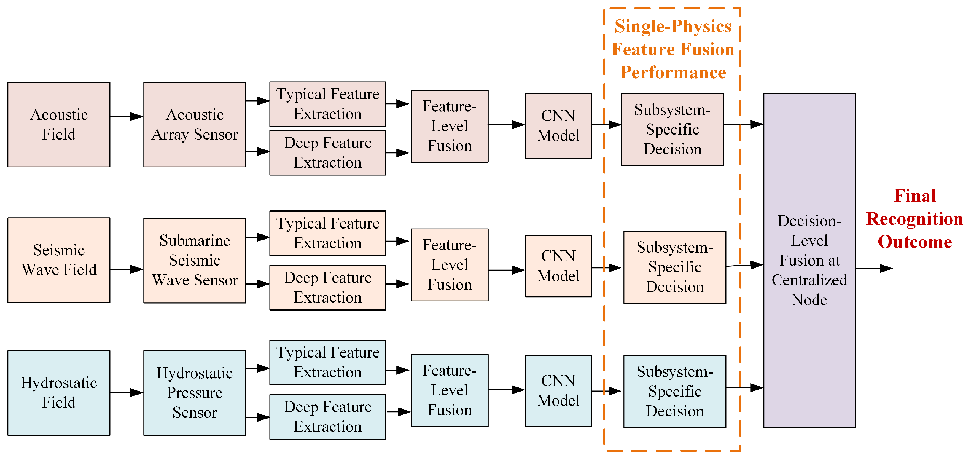
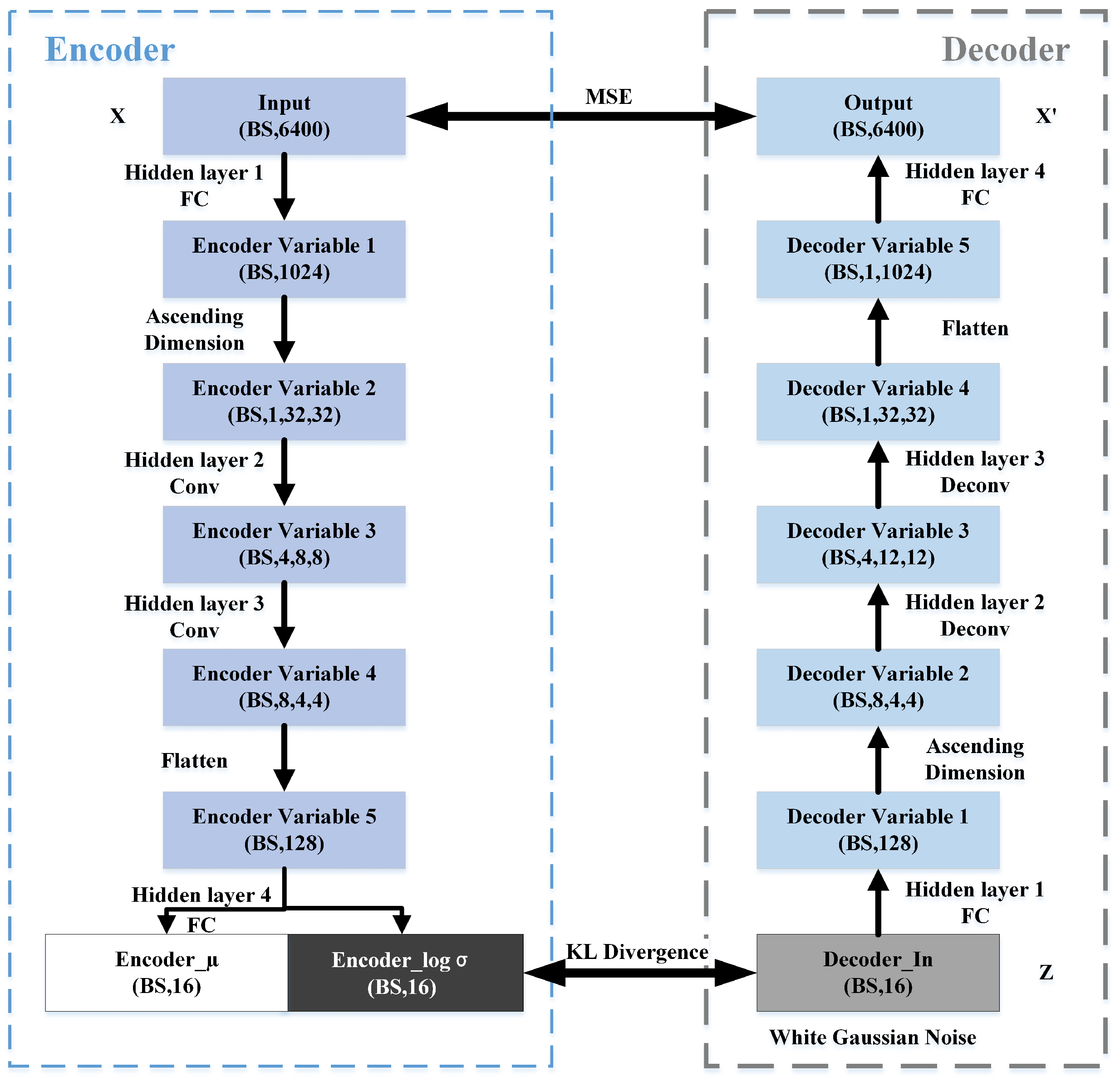
To tackle these challenges, this paper integrates deep learning and information fusion theory to propose a multi-level fusion perception method for underwater targets. We design an intelligent network fusion framework for underwater target recognition, incorporating both feature-level and decision-level fusion across multiple physical fields, including acoustic, pressure, and seismic fields. An autoencoder-based network is employed to extract deep features of underwater targets, which are then fused with conventional typical features to form a multi-dimensional heterogeneous feature set. Furthermore, neural network-based classification models are developed for each physical field subsystem. To address class imbalance and varying sample difficulty, we introduce a C-Focal Loss function tailored to the three underwater target categories. Finally, we propose an evidence-theoretic network fusion framework and a neural network-based DS evidence fusion algorithm to achieve deep fusion perception of underwater targets.

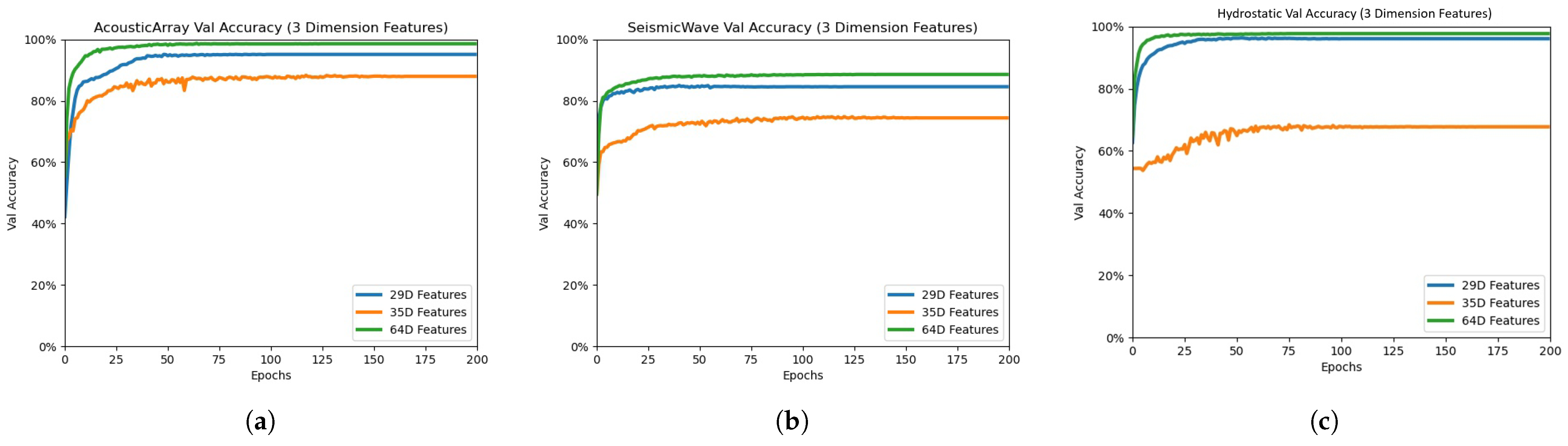
The remainder of this paper is structured as follows. Section 2 investigates underwater target recognition using multi-physical-field sensing and introduces an intelligent fusion recognition framework based on multiple sensor modalities. Section 2.1 presents a single-physical-field feature-level fusion approach, extracting multi-dimensional typical features and employing a variational autoencoder network to extract deep features and forming a comprehensive fusion feature set for subsequent classification. 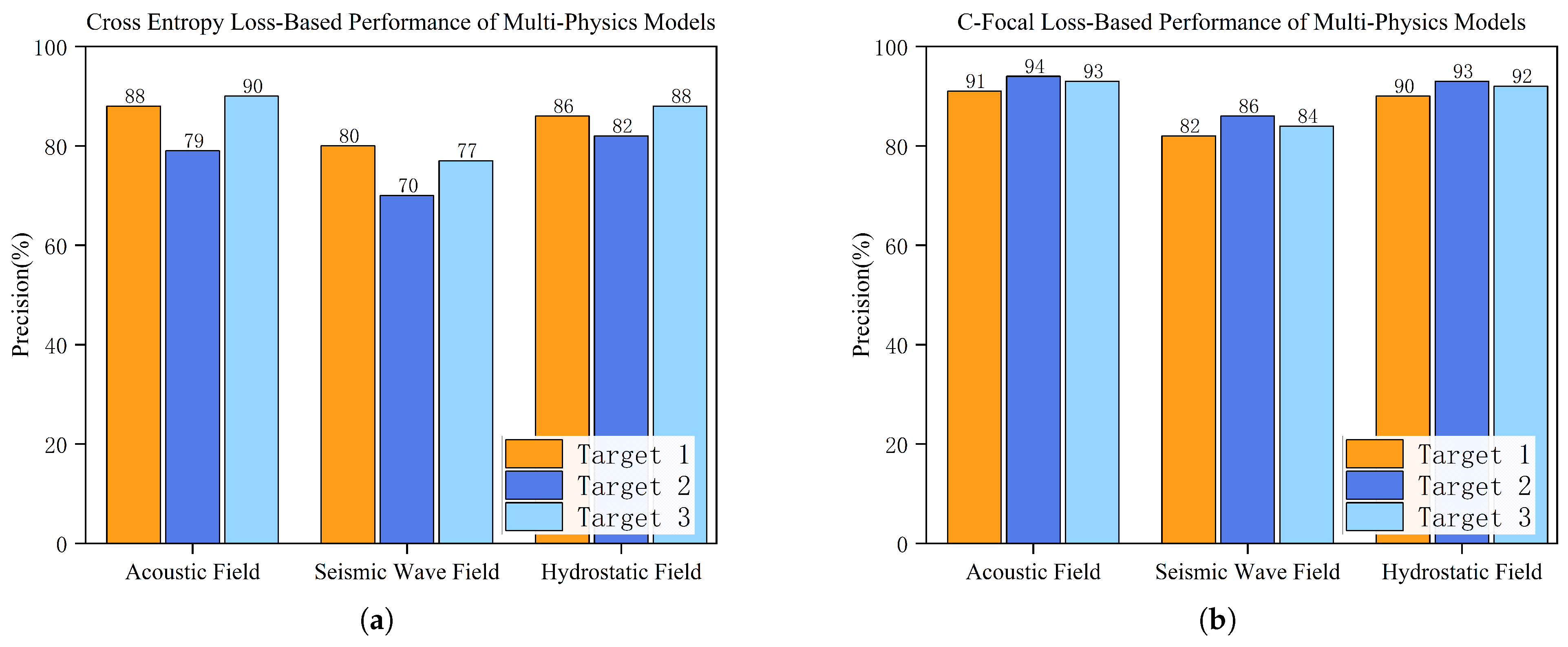Section 2.2 develops neural network models for each physical field subsystem and introduces the C-Focal Loss function to address sample imbalance among the three target categories. 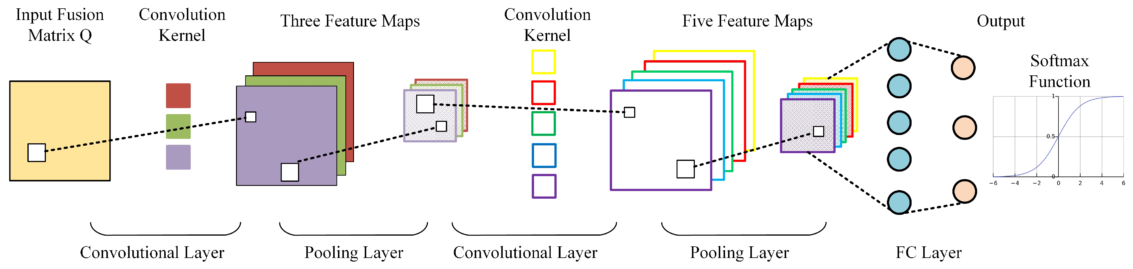Section 2.3 explores multi-physical-field decision fusion using evidence theory and proposes an evidence-theoretic network fusion architecture and algorithm. 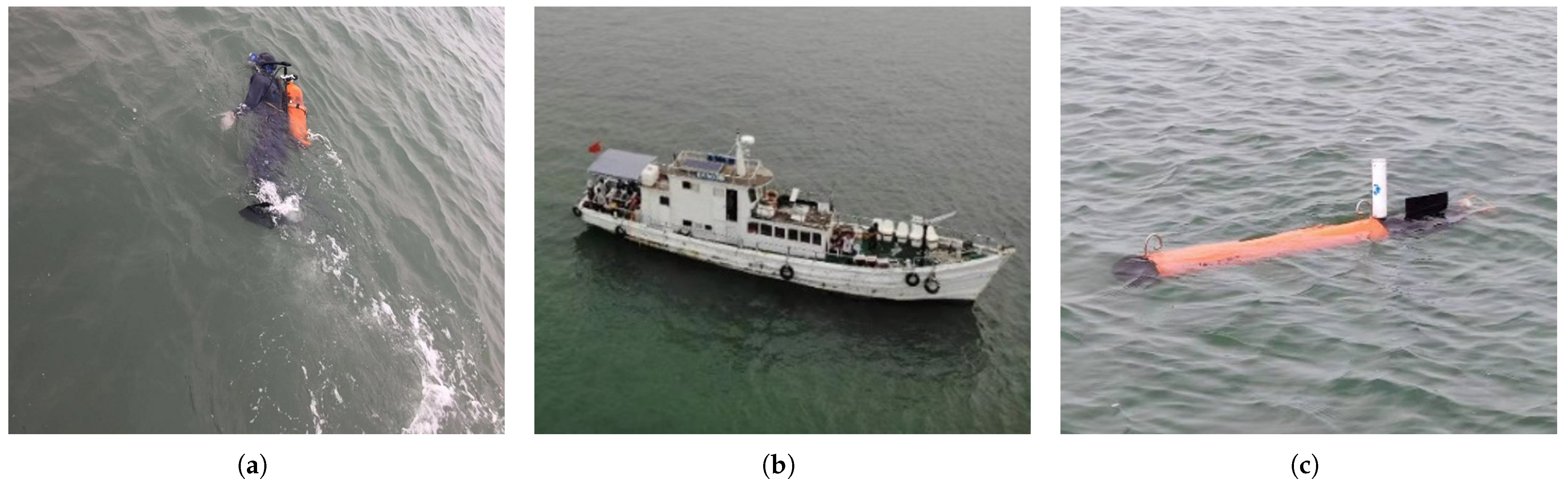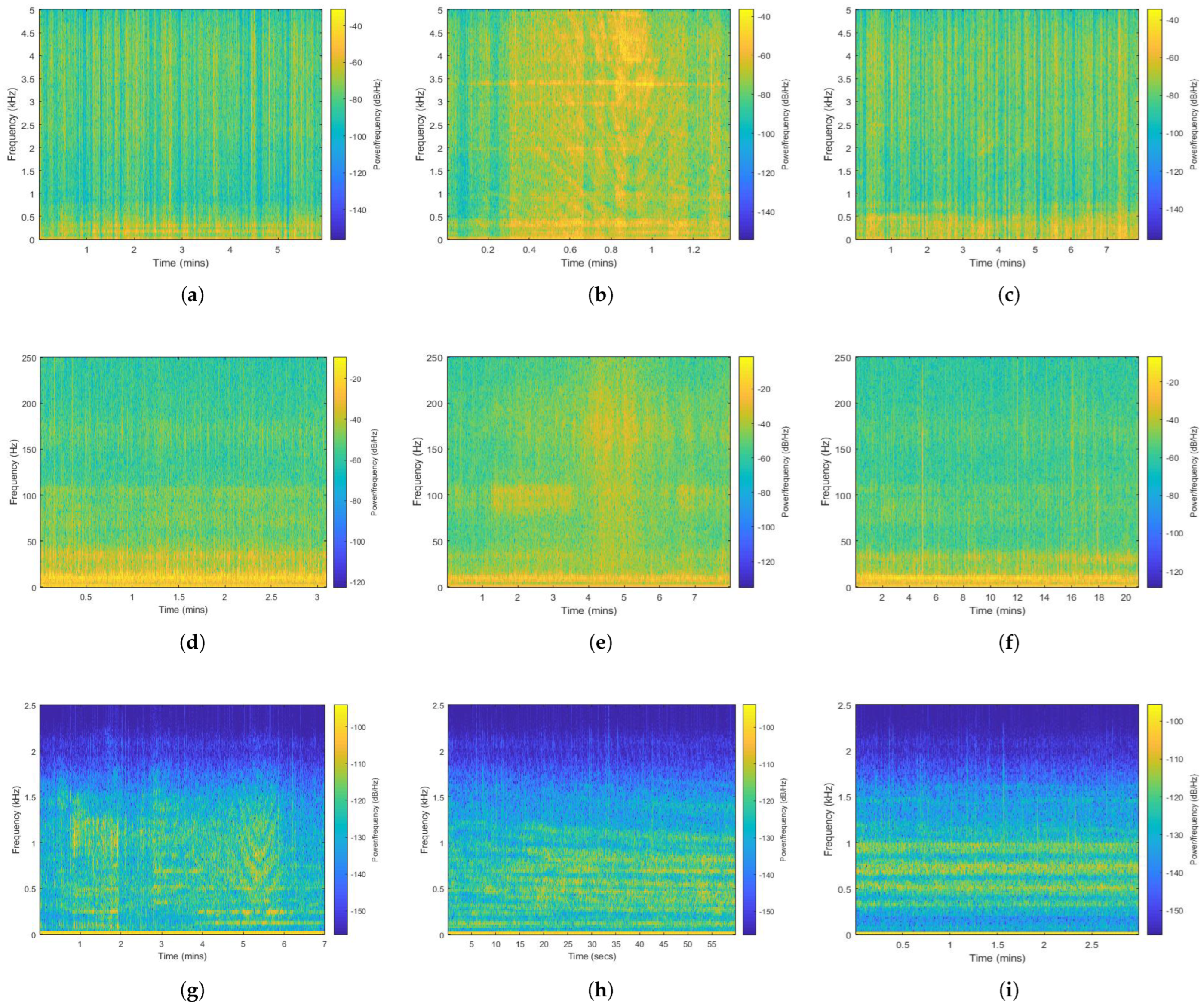Section 3 presents experimental validation using real-world signals, including the construction of a multi-physical-field signal acquisition system, comparative classification results of individual subsystems, and decision-level fusion at the fusion center. Performance analysis across different physical fields is conducted to verify the effectiveness of the proposed approach.

2. Methods

2.1. Fusion Recognition Framework for Underwater Targets

To fully leverage the multi-physical-field information of underwater targets, a multi-physical-field-based fusion intelligent perception model is developed, as shown in Figure 1. First, three types of sensors are used to receive underwater target signal data. Based on the extraction of typical features from multi-physical-field underwater target signals, an autoencoder network model is constructed to extract deep features from the multi-physical-field signals. Feature-level fusion is then performed within each individual physical field. Next, a convolutional neural network (CNN) model is established for classification and recognition based on feature-level fusion within each physical field. Finally, a neural network-driven Dempster–Shafer (NNDS) evidence fusion framework and an algorithm are proposed. Decision-level fusion is carried out at the fusion center to achieve the intelligent multi-physical-field fusion perception of underwater targets.

2.2. Single-Physics Feature-Level Fusion for Underwater Targets

2.2.1. Characteristic Feature Extraction of Underwater Target Signals

A total of 35 features were extracted as typical characteristics of underwater target signals, including time-domain waveform features, frequency-domain analysis features, statistical features, auditory features, and nonlinear characteristics. The numerical indices and corresponding names of the 35-dimensional typical features used in this study are listed in

Table 1. Typical feature extraction.

Feature Number	Feature Name
1	Energy
2	Zero-crossing rate
3	Energy entropy
4	Spectral centroid
5	Spectral width
6	Spectral entropy
7	Spectral flux
8	Spectrum roll-off
9–21	Mel-frequency Cepstrum coefficients
22	Harmonic ratio
23	Fundamental frequency
24–35	Chromaticity vectors

.

2.2.2. VAE-Based Deep Feature Extraction for Underwater Targets

The core concept of extracting deep signal features using a variational auto-encoder (VAE) model involves constraining the model’s output through reconstruction loss and distribution loss. Real target signals are fed into the VAE, and the feature vectors from the intermediate hidden layers of the encoder–decoder architecture are extracted as deep features. As shown in Figure 2, the variational auto-encoder structure comprises two components: an encoder and a decoder. The VAE model consists of two parts: an encoder and a decoder. Both components contain four hidden layers. In the encoder, the first and fourth layers are fully connected layers. The second and third layers are convolutional layers. The decoder mirrors the encoder’s architecture. The final layer of the encoder was set to 29 dimensions.

The loss function of the VAE model is composed of two terms: the reconstruction error and the distribution error. The reconstruction error evaluates the difference between the generated synthetic signals and the input real signals, while the distribution error quantifies the divergence between the probability distribution of the random noise input to the decoder and the encoder’s output distribution (characterized by mean and log variance). Minimizing these errors ensures that the extracted deep features retain critical signal information. It also enforces a unified probability distribution for these features. The reconstruction loss is calculated using the mean squared error (MSE), as defined in Equation (1). The distribution loss is computed via Kullback–Leibler (KL) divergence, as shown in Equation (2).

$${Loss}_{MSE}\left(X^{\prime },X\right)={\displaystyle \frac{1}{N}}\sum _{i=1}^N{\left(x^{\prime }\left(t\right)-x\left(t\right)\right)}^2$$

(1)

$$Los{s}_{KL}\left(p\right|q)=\int p\left(x\right)log\left({\displaystyle \frac{p\left(x\right)}{q\left(x\right)}}\right)dx$$

(2)

where $x\left(t\right)$ is true signals, $x^{\prime }\left(t\right)$ is simulation signals, and X and $X^{\prime }$ are the sets of two kinds of signals. $p\left(x\right)$ and $q\left(x\right)$ are the probability distribution that the output of the encoder obeys and the probability distribution to be approximated, respectively.

For each type of target in the three physical fields, a corresponding autoencoder model is designed, with the latent variable set to 29 dimensions, enabling the extraction of 29–dimensional deep features from the signals. This includes three models based on the acoustic field targets, three models based on the seismic wave-field targets, and three models based on the pressure field targets, making a total of nine models. These nine models are trained separately according to the algorithmic process outlined in Algorithm 1, enabling the extraction of deep features from the signals of the three types of targets in each physical field.

Algorithm 1 Underwater target deep feature extraction algorithm
Input: Measured signal sample $X=\{x_i\in R^d{\}}_{i=1}^n$, batch size $BS$, learning rate $Lr$, maximum iteration count $Epoch$
Output: Deep feature vector Z
1:	Initialize current iteration count $e=0$, network parameters W and b with random values
2:	while $e<Epoch$ do
3:	Perform forward propagation. Compute latent variable Z and reconstructed $X^{\prime }$
4:	Calculate the loss ${\mathcal{L}}_{\mathrm{Re}con}={\displaystyle \frac{1}{N}}{\sum }_{n=0}^{N-1}{∥X_n-{X^{\prime }}_n∥}^2$, ${\mathcal{L}}_{dis}=log\left({\displaystyle \frac{1}{{\sigma }_Q}}\right)+{\displaystyle \frac{1}{2}}({\sigma }_Q^2+{\mu }_Q^2)-{\displaystyle \frac{1}{2}}$
5:	Perform backward propagation and update parameters W and b based on the loss
6:	Dynamically adjust learning rate $Lr$ and batch size $BS$
7:	Increment the iteration count $e=e+1$
8:	return Final deep feature vector Z

2.2.3. Multi–Dimensional Feature Fusion Method for Underwater Targets

The target feature information was fused using covariance matrices. The 64–dimensional feature set combined 35–dimensional typical features and 29–dimensional deep features from various signals. This integration generated the multi–feature fused covariance matrix Q.

$$Q={\displaystyle \frac{1}{n+1}}\sum _{k=1}^N\left(z_k-\mu \right){\left(z_k-\mu \right)}^T$$

(3)

where $z_k$ is the typical feature and deep feature vector, and the total number of vectors is the feature dimension 64, where $\mu ={\displaystyle \frac{1}{n+1}}{\sum }_{k=1}^N{z}_k$

$$\left[\begin{array}{cccc}{c}_{11}& c_{12}& \dots & c_{1N}\\ c_{21}& c_{22}& \dots & c_{2N}\\ \dots & \dots & \dots & \dots \\ c_{N1}& c_{N2}& \dots & c_{NN}\end{array}\right]$$

(4)

As shown in Equation (4), the final covariance matrix, Q, is presented. The diagonal entries represent the variance of individual features. Off-diagonal elements indicate cross-correlations between distinct features. The covariance matrix dimension is determined solely by the feature count, resulting in a $64\times 64$ positive definite matrix, Q. Furthermore, Q exhibits an inherent noise-filtering capability and enhanced robustness.

2.3. C-Focal Loss-Based Neural Network Classification Model

For each physical field, a subsystem neural network classifier is constructed. The fused feature matrix is used as input to the convolutional neural network (CNN). The CNN consists of three convolutional layers, where the number of filters in each layer is 3, 5, and 10, respectively. After each convolutional layer, batch normalization is applied to promote network convergence, improve accuracy, and reduce overfitting, allowing for a higher learning rate. Subsequently, a pooling layer is added to reduce the dimensionality. Finally, two fully connected layers with 10 and 3 units are connected, respectively. The output layer uses the softmax function, which maps the classification output probabilities to the range [0, 1] and ensures that the probabilities sum to 1. The final multi-physical-field subsystem convolutional neural network classification model constructed in this paper is shown in Figure 3. The main parameters of the model are listed in

Table 2. Parameters of CNN Model.

Parameters	Settings
Convolution stride	1
Convolution kernel size	3 × 3
Activation function	ReLU
Optimizer	Adam
Loss function	C-Focal Loss
Pooling layer	Max pooling
Pooling size	2 × 2
Pooling stride	2
Learning rate	[0.01, 0.004, 0.001, 0.0004, 0.0001]
Batch size	[16, 32, 64, 128]

.

Due to the significant differences in the number of data samples collected for the three target categories across different physical fields, the difficulty in recognizing the three target categories varies. To address the issues of class imbalance and easy-to-classify versus difficult-to-classify samples, a C-Focal Loss function tailored to underwater target classification is designed. This function adjusts the weights of the cross-entropy loss to make the model focus more on hard-to-classify samples during the training process, rather than being dominated by a large number of easy-to-classify samples.

$$\mathrm{FL}\left(p_c\right)=-{\alpha }_c{(1-p_c)}^{\gamma }log\left(p_c\right)$$

(5)

where $p_c$ is the model’s predicted probability for each target category, $p_c\in {[0,1]}^C$, and C is the total number of categories. ${\alpha }_c$ is the balancing sample weight coefficient. $\gamma$ is the focusing parameter that controls the adjustment of the loss weights for easy and difficult samples. The larger $\gamma$ is, the more the loss weight for easy samples is reduced, making the model focus more on difficult samples.

To address the imbalance of the three target categories in each physical field, the sample weight coefficient ${\alpha }_c$ is adjusted to regulate the contribution of different category samples to the loss function. Through calculation based on Equation (6), followed by normalization, the balanced sample weight coefficients for the corresponding physical field can be obtained.

$${\alpha }_c={\displaystyle \frac{1}{f_c}}$$

(6)

where $f_c$ is the frequency of the three target categories. The balancing sample weight coefficients for the C-Focal Loss function in the neural network models for the three physical fields are computed as follows: for the acoustic field, ${\alpha }_c=(0.22,0.66,0.12)$; for the seismic wave field, ${\alpha }_c=(0.19,0.49,0.32)$; and for the hydroacoustic pressure field, ${\alpha }_c=(0.24,0.61,0.15)$.

To address the issue of varying difficulty levels of sample categories in this study, the focusing parameter $\gamma$ is set to 2. As $p_c$ approaches 1,${(1-p_c)}^r$ approaches 0, and the loss contribution is reduced. When $p_c$ is small, ${(1-p_c)}^r$ approaches 1, and the loss weight remains nearly unchanged. This effectively reduces the weight for samples with high prediction accuracy and increases the weight for samples with lower prediction probabilities.

2.4. Neural Network-Based Multi-Physics Dempster-Shafer Evidence Fusion

For subsystem decisions derived from individual physical fields, decision-level fusion was performed using Dempster-Shafer evidence theory. A neural network-enhanced Dempster-Shafer evidence fusion algorithm was developed. The collected information from each physical field was converted into basic probability assignment (BPA) functions. Subsequently, the Dempster combination rule was applied to fuse multiple BPAs, yielding an updated fused BPA. Ultimately, the final decision was generated based on the fusion results.

In pattern recognition, the confusion matrix mathematically characterizes the correspondence between ground-truth labels and predicted classifications, serving as a widely adopted evaluation metric. The recognition rates derived from confusion matrices can be utilized as prior knowledge to quantify classifier-specific confidence levels. This probabilistic information enables weighted fusion during BPA construction, enhancing the reliability of evidence integration.

First, the final confusion matrices of each neural network classifier were obtained from the validation set. The local confidence levels for individual classification outcomes were computed per classifier.

$$F_l\left(i\right)=c_{ii}/\sum _{j=1}^k{c}_{ji}$$

(7)

where $c_{ji}$ quantifies the number of samples for which the ground-truth class, j, is predicted as category i, and k represents the total number of underwater target categories. Both parameters are algorithmically extracted from the validation set confusion matrix, $C_l$.

$$C_l=\left[\begin{array}{cccc}{c}_{11}& c_{12}& \dots & c_{1k}\\ c_{21}& c_{22}& \dots & c_{2k}\\ \dots & \dots & c_{ji}& \dots \\ c_{k1}& c_{k2}& \dots & c_{kk}\end{array}\right]$$

(8)

During test-set evaluations, let $P_l\left(i\right)$ denote the output probability of the l classifier assigning the i class. The basic probability assignment (BPA) was formulated by integrating validation-derived confidence measures with test-set probabilities, $P_l\left(i\right)$.

$$m_l\left(i\right)=P_l\left(i\right)F_l\left(i\right)$$

(9)

The local confidence measure, $F_l\left(i\right)$, quantifies the classification certainty for category i generated via the l neural network classifier.

Next, evidence fusion theory was employed to calculate synthetic confidence measures across multi-physical-field subsystems.

$$Z\left(i\right)={\displaystyle \frac{1}{N}}\prod _{l=1}^L{m}_l\left(i\right)$$

(10)

$$N=\sum _{i=1}^k\left[\prod _{l=1}^L{m}_l\left(i\right)\right]$$

(11)

where N is the normalization factor of probabilistic scaling consistency, L denotes the sensor-type cardinality, and k represents the total number of underwater target classes.

The final decision–level fusion output determined the underwater target category, $\widehat{i}$, through maximum synthetic confidence measures, $Z\left(i\right)$.

$$\widehat{i}=arg\underset{i}{max}\left[Z\left(i\right)\right]$$

(12)

The classification and recognition of underwater targets at the decision-level fusion stage across marine multi-physical field subsystems can be performed via the Neural network Dempster-Shafer evidence fusion algorithm workflow demonstrated in Algorithm 2.

Algorithm 2 Neural network Dempster-Shafer evidence fusion algorithm
Input: Validation set confusion matrices $C_1$, $C_2$, $C_3$ from three physical-field subsystems, and multi-physical-field test signal S
Output: Prediction target class label $\widehat{i}$
1:	Calculate the local confidence measures $F_l\left(i\right)$ across the three subsystem classifiers for each classification outcome
2:	Extract typical features and deep features separately from test signal S, then feed the multi-feature fused covariance matrix Q into the pre-trained neural network
3:	Generate output probability $P_l\left(i\right)$ for the i target category during neural network test set classification
4:	Compute the Basic Probability Assignment $m_l\left(i\right)=P_l\left(i\right)F_l\left(i\right)$
5:	Calculate the synthetic confidence measures $Z\left(i\right)={\displaystyle \frac{1}{N}}{\prod }_{l=1}^L{m}_l\left(i\right)$ of different physical field subsystems
6:	Find the $\widehat{i}$ that maximizes the synthetic confidence measures
7:	return $\widehat{i}$

3. Results

3.1. Multi-Physics Signal Acquisition and Analysis for Underwater Targets

To acquire multi-physical field observation data for underwater targets, we established three distinct sensor acquisition systems targeting acoustic, seismic wave, and hydrostatic pressure fields, respectively. As shown in Figure 4a, the acoustic array sensor system was suspended on the side of the research vessel to capture high-frequency acoustic signatures from aquatic targets with a sampling rate of 10 kHz. Figure 4b illustrates the seismic wave sensor system deployed on the seafloor, specifically designed to record ultra-low-frequency seismic signals propagating through submarine strata at a 500 Hz sampling rate. The pressure sensing unit in Figure 4c, consisting of high-precision transducers submerged near the seabed, monitors hydrodynamic pressure variations induced via moving underwater targets with a 5 kHz sampling capability. This tri-physical-field configuration leverages complementary detection mechanisms: the acoustic system excels in near-surface target characterization, and the seismic array provides deep structural vibration signatures, while the pressure sensors capture transient fluid disturbances.

Marine trials were conducted in Jiaozhou Bay in the Yellow Sea, China. Three types of underwater sensors were deployed to collect signals from three distinct mobile underwater targets. As illustrated in Figure 5, the targets comprised the following: Target 1—submersible combat divers, Target 2—a research vessel, and Target 3—an unmanned underwater vehicle (UUV).

The acquired acoustic, seismic, and hydrostatic pressure signals from multiple sensors underwent preprocessing that included spatiotemporal synchronization, low-pass filtering, normalization, and framing/windowing. Since the classification task focuses on low-signature targets, samples were categorized based on a 500-m proximity threshold (targets within 500 m of the observation system were labeled as valid samples).

Table 3. Sample sizes of different targets across physical fields.

Category	Acoustic Field	Seismic Wave Field	Hydrostatic Pressure Field
Target 1	2476	6113	3597
Target 2	838	2516	1434
Target 3	4445	3717	5992

summarizes the effective sample counts for each target category across the three physical fields.

To further verify the reliability of signal labeling, time-frequency analysis was conducted on the signals of the three target types collected from different physical fields. The corresponding time-frequency spectrograms are shown in Figure 6.

It can be observed that, in the time-frequency spectrograms of the acoustic field for the three target types, distinct spectral line signals are present for each target, with unique spectral characteristics for each type. This confirms the reliability of the signal labeling criteria. Notably, Target 2 exhibits prominent harmonic signals, suggesting that target characteristics are more distinct in the acoustic field.

In the time–frequency spectrograms of the seismic wave field, some unique signals can also be identified, though they are less distinct. This indicates the need for more effective feature extraction techniques or deep neural networks to extract high-level features. Similarly, in the time–frequency spectrograms of the hydroacoustic field, relatively clear target signal spectral lines can be observed. However, the signals of the three targets appear quite similar, necessitating the design of an efficient classifier for accurate target classification.

The dataset for each physical field is split into training, validation, and test sets at a 7:2:1 ratio. The neural network model is first trained using the training set. The validation set is then used to fine-tune hyperparameters such as the learning rate of the convolutional neural network, with the final model parameters determined based on the highest classification accuracy on the validation set. Lastly, the trained models are evaluated on the test set to generate subsystem decisions for each physical field.

3.2. Subsystem-Specific Neural Network Classification Across Multi-Physics Domains

3.2.1. Comparison of Recognition Results with Different Feature Inputs

For the acoustic field sensing subsystem, hydroacoustic field sensing subsystem, and seismic wave field sensing subsystem, classification experiments were conducted using typical features, deep features, and fused features as network inputs. The typical and deep features were processed through an inner product operation to form a two-dimensional feature matrix. The deeply fused features utilize a fused positive definite matrix as the network input, enabling the training and testing of the neural network model.

Table 4. Input dimensions of different features.

Input Feature	Input Dimension
Fused feature matrix	64 × 64
Typical feature matrix	35 × 35
Deep feature matrix	29 × 29

presents a comparison of input dimensions for different feature types.

From the table, it can be seen that the input dimension of the fused features is the highest, while the input dimension of the deep features is the lowest. Each feature undergoes 20 sets of experiments with different batch sizes (16, 32, 64, and 128) and learning rates (0.01, 0.004, 0.001, 0.0004, and 0.0001), making a total of 60 sets of experiments for the three features. After the network model is trained, the accuracy of the training and validation sets is compared to obtain the optimal network parameters and model for each feature. These network parameters are then used for testing, yielding the results for the test set.

In the acoustic field, seismic wave field, and hydrodynamic field sensor subsystems, typical feature matrices, deep feature matrices, and fused feature matrices are used as inputs to train the CNN model. The optimal hyperparameters of the neural network model are selected based on the validation set results. Finally, when the typical features are used as input, the model parameters are set to $Lr=0.001$ and $BS=64$; when deep features and fused features are used as inputs, the model parameters are set to $Lr=0.0004$ and $BS=64$.

From the performance comparison of the classification models in each physical field shown in Figure 7, it can be observed that, in each physical field subsystem, the network model trained with typical features achieves the lowest classification performance. The network model trained with deep features performs better, and the network model trained with fused features achieves the highest classification performance. This indicates that the approach of training models with fused features, as proposed in this study, is effective.

Additionally, it can be observed that the acoustic field subsystem’s corresponding model achieves the highest accuracy, with the classification performance reaching approximately 95%. In the seismic wave field and hydrodynamic field subsystems’ validation set classification results, the best classification performance is achieved with fused features, while the classification performance with typical features is relatively poor. This suggests that some typical features extracted from acoustic signals may not be applicable to seismic wave field and hydrodynamic field signals, resulting in lower classification accuracy. However, deep features achieve good classification performance, compensating for the shortcomings of typical features.

3.2.2. Comparison of Recognition Results with Different Loss Functions

Using the same fused features as the network model input, a comparison is made between the classification recognition effects of the C-Focal Loss and Cross Entropy Loss functions. Each physical field subsystem neural network model is tested on the test set. To analyze the model’s recognition performance for each target class, classification precision is used as the evaluation metric for individual subsystems. Figure 8 shows the classification precision test results of each physical field subsystem model under the two loss functions.

Cross Entropy Loss-Based Performance of Multi–Physics Models The test results from different subsystem models reveal that, similar to the validation set results, the classification accuracy of the sonar subsystem model is consistently higher than that of the seismic wave and hydroacoustic pressure field subsystems. This suggests that sonar signals contribute more significantly to the classification and recognition of the three types of underwater targets. When the classification performance under two loss functions is compared, it is observed that models using cross-entropy loss exhibit the lowest recognition accuracy for target 2 in each physical field. This is because target 2 has the fewest samples, resulting in the poorest classification performance. In contrast, target 3 has the largest number of samples in both the sonar and hydroacoustic pressure fields, which leads to the highest classification accuracy for this target in the corresponding models. Additionally, in the seismic wave field, target 1, which has the largest sample size, achieves the highest classification accuracy. This indicates that, under imbalanced sample conditions, the classification performance of the model using cross-entropy loss is influenced by the number of samples per target.

Based on the comparison of test results, the C-Focal Loss designed in this paper effectively addresses the class imbalance issue. The models using C-Focal Loss generally show superior performance over those using cross-entropy loss, especially for target 2, which has the fewest samples. The models with C-Focal Loss achieve the highest recognition accuracy for target 2 across all physical field subsystems, thereby validating the effectiveness of the proposed C-Focal Loss.

3.3. Decision-Level Fusion Classification Results in Multi-Sensor Systems

After the respective decision results from the three subsystems were obtained, a decision-level fusion of the three sensor subsystems was performed at the network fusion center. The final classification result was obtained through the NNDS algorithm proposed in this paper. This result was then compared with the classification performance of the Multi-Physical Field Feature Network Fusion (MPNF) method and the Subsystem Voting Decision Fusion (SVDF) method. The Multi-Physical Field Feature Network Fusion method refers to directly inputting all features from the multi-physical fields into the network, with the neural network leveraging its learning capability to perform fusion and classification. The Subsystem Voting Decision Fusion method involves quantifying the decision results of each subsystem into 1–bit values, followed by majority voting at the fusion center to achieve the final classification.

For underwater multi-target classification, accuracy, macro-precision, macro-recall, and macro F1 score are used for comparative evaluation.

Table 5. Comparison of fusion-system classification results.

Fusion Method	Accuracy	Macro Precision	Macro Recall	Macro F1
MPNF	82.48%	82.81%	82.95%	82.88%
SVDF	88.45%	86.26%	88.25%	87.19%
NNDS	97.15%	96.24%	96.73%	96.48%

shows the overall classification results of the three fusion systems in the test set. The results presented are the average values with standard deviations obtained from 10–fold cross-validation experiments, which effectively ensure the statistical reliability of the performance evaluation.

The comparison of classification results using the three fusion methods shows that both decision-level fusion methods outperform the multi-physical field feature network fusion method. This indicates that, for the underwater target data in this study, directly using network fusion to replace feature and decision fusion is not effective or that the dataset size in this study is insufficient to support the training of direct network fusion across multiple physical fields. The evidence theory network fusion decision algorithm proposed in this paper demonstrates better performance on all four evaluation metrics compared to the subsystem hard-decision voting method. It is more suitable for multi-physical field underwater target classification and recognition, thus validating the effectiveness of the proposed NNDS.

4. Discussion

The multi-physical field deep fusion perception method proposed in this paper considers imbalanced sample distributions across underwater target signal acquisitions through independent decision-making by physical field subsystems. Each physical field operates through mutually independent subsystem recognition systems, effectively reducing cross-physical-field signal interference. Within each subsystem’s neural network classifier, we implement feature fusion between typical signal characteristics and VAE-generated deep features, facilitating a comprehensive extraction of multi-dimensional heterogeneous characteristics from individual samples to enhance classification capability. A dedicated C-Focal Loss function is designed to address inter-class imbalance in practical underwater target sample collections, significantly enhancing single subsystem recognition accuracy. Finally, decision-level fusion via the NNDS algorithm further optimizes the multi-physical field recognition system’s performance. This hierarchical fusion architecture—spanning sample processing, feature extraction, and decision integration—ultimately achieves 97.15% accuracy in multi-physical field underwater target recognition, demonstrating the framework’s technical superiority.

However, this paper faced certain limitations. From a multi-physics perspective, this study focused on acoustic, seismic, and hydrostatic pressure fields due to limitations in experimental equipment and data availability. Future work should incorporate underwater magnetic and electric fields to comprehensively extract multi-physics signatures of submerged targets. Subsequent research priorities include developing rapid multi-physics fusion-recognition techniques to achieve more efficient and accurate underwater target perception across broader physical domains.

From practical deployment perspectives, underwater surveillance primarily involves detecting uncharacterized targets, particularly non-cooperative platforms like UUVs where pre-collected training data are unavailable. Future research should prioritize investigating few-shot and zero-shot intelligent perception paradigms, leveraging meta-learning architectures or cross-domain transfer mechanisms to enable the precise classification of unidentified non-cooperative underwater targets with limited supervision, demonstrating superior generalization capabilities under extreme data scarcity conditions.

5. Conclusions

This paper has addressed the challenges of multi-physics signal fusion for underwater targets and low classification accuracy caused by sample imbalance. Integrating deep learning with information fusion theory, we proposed a deep multi-physics fusion perception method under imbalanced data conditions. An intelligent network architecture was developed for underwater target recognition, incorporating variational autoencoder (VAE) models to extract deep features from targets. These deep features were fused with typical features at the feature level to form multi-dimensional heterogeneous representations. Subsystem-specific neural classifiers were constructed for each physical field. To mitigate inter-class imbalance and hard–easy sample disparity across three target categories, a customized C-Focal Loss function was designed. An NNDS fusion algorithm was further proposed and validated through comparative experiments using real-world datasets.

Experimental results from marine trials demonstrate that the proposed feature fusion framework combining typical and deep features significantly enhances classification performance across three physical fields. Recognition accuracy using fused features exceeded 80% in all physical fields, outperforming individual feature-based approaches and thereby validating the efficacy of intra-physics feature fusion for underwater target identification. C-Focal Loss achieved a 10% improvement over cross-entropy loss, particularly boosting precision for minority-class targets, demonstrating its effectiveness in handling class imbalance. The proposed NNDS fusion algorithm attained 97.15% recognition accuracy, surpassing the Multi-Physical Field Feature Network Fusion (MPNF) and the Subsystem Voting Decision Fusion (SVDF) methods, with enhanced confidence levels and robustness against sensor noise.

References

1. Joshi, R.; Usmani, K.; Krishnan, G.; Blackmon, F.; Javidi, B. Underwater object detection and temporal signal detection in turbid water using 3D-integral imaging and deep learning. Opt. Express 2024, 32, 1789–1801. [Google Scholar] [CrossRef]
2. Huang, C.; Zhao, J.; Zhang, H.; Yu, Y. Seg2Sonar: A full-class sample synthesis method applied to underwater sonar image target detection, recognition, and segmentation tasks. IEEE Trans. Geosci. Remote Sens. 2024, 62, 1–19. [Google Scholar] [CrossRef]
3. Luo, X.; Chen, L.; Zhou, H.; Cao, H. A survey of underwater acoustic target recognition methods based on machine learning. J. Mar. Sci. Eng. 2023, 11, 384. [Google Scholar] [CrossRef]
4. Luo, R.; Li, C.; Wang, F. Underwater motion target recognition using artificial lateral line system and artificial neural network method. Ocean. Eng. 2024, 303, 117757. [Google Scholar] [CrossRef]
5. Chen, J.; Han, B.; Ma, X.; Zhang, J. Underwater target recognition based on multi-decision lofar spectrum enhancement: A deep-learning approach. Future Internet 2021, 13, 265. [Google Scholar] [CrossRef]
6. Er, M.J.; Chen, J.; Zhang, Y.; Gao, W. Research challenges, recent advances, and popular datasets in deep learning-based underwater marine object detection: A review. Sensors 2023, 23, 1990. [Google Scholar] [CrossRef]
7. Ghamisi, P.; Rasti, B.; Yokoya, N.; Wang, Q.; Hofle, B.; Bruzzone, L.; Bovolo, F.; Chi, M.; Anders, K.; Gloaguen, R.; et al. Multisource and multitemporal data fusion in remote sensing: A comprehensive review of the state of the art. IEEE Geosci. Remote. Sens. Mag. 2019, 7, 6–39. [Google Scholar] [CrossRef]
8. Chen, D.; Liu, Z.; Wang, L.; Dou, M.; Chen, J.; Li, H. Natural disaster monitoring with wireless sensor networks: A case study of data-intensive applications upon low-cost scalable systems. Mob. Netw. Appl. 2013, 18, 651–663. [Google Scholar] [CrossRef]
9. Corke, P.; Wark, T.; Jurdak, R.; Hu, W.; Valencia, P.; Moore, D. Environmental wireless sensor networks. Proc. IEEE 2010, 98, 1903–1917. [Google Scholar] [CrossRef]
10. Yong, J.; Zhu, R.Q. Research on decision fusion in underwater target recognition. In Proceedings of the 2nd International Conference on Information Science and Engineering, Hangzhou, China, 4–6 December 2010; IEEE: New York, NY, USA, 2010; pp. 2334–2337. [Google Scholar]
11. Jie, X.; Jinfang, C.; Guangjin, H.; Xiudong, Y. A neural network recognition model based on ship acoustic-magnetic field. In Proceedings of the 2011 Fourth International Symposium on Computational Intelligence and Design, Hangzhou, China, 28–30 October 2011; IEEE: New York, NY, USA, 2011; Volume 1, pp. 135–138. [Google Scholar]
12. Pan, X.; Sun, J.; Feng, T.; Lei, M.; Wang, H.; Zhang, W. Underwater target recognition based on adaptive multi-feature fusion network. Multimed. Tools Appl. 2024, 84, 7297–7317. [Google Scholar] [CrossRef]
13. Teng, B.; Zhao, H. Underwater target recognition methods based on the framework of deep learning: A survey. Int. J. Adv. Robot. Syst. 2020, 17, 1729881420976307. [Google Scholar] [CrossRef]
14. Han, X.C.; Ren, C.; Wang, L.; Bai, Y. Underwater acoustic target recognition method based on a joint neural network. PLoS ONE 2022, 17, e0266425. [Google Scholar] [CrossRef] [PubMed]
15. Zhang, Q.; Da, L.; Zhang, Y.; Hu, Y. Integrated neural networks based on feature fusion for underwater target recognition. Appl. Acoust. 2021, 182, 108261. [Google Scholar] [CrossRef]
16. Zhang, S.; Wang, C.; Sun, Q. Underwater target noise recognition and classification technology based on multi-classes feature fusion. Xibei Gongye Daxue Xuebao/J. Northwestern Polytech. Univ. 2020, 38, 366–376. [Google Scholar] [CrossRef]
17. Cao, X.; Zhang, X.; Togneri, R.; Yu, Y. Underwater target classification at greater depths using deep neural network with joint multiple-domain feature. IET Radar Sonar Navig. 2019, 13, 484–491. [Google Scholar] [CrossRef]
18. Dong, Y.; Zhang, G.; He, X.; Tang, J. Information fusion in networked underwater target detection. In Proceedings of the OCEANS 2015, Genova, Italy, 18–21 May 2015; IEEE: New York, NY, USA, 2015; pp. 1–4. [Google Scholar]
19. Fei, T.; Kraus, D.; Zoubir, A.M. Contributions to automatic target recognition systems for underwater mine classification. IEEE Trans. Geosci. Remote. Sens. 2014, 53, 505–518. [Google Scholar] [CrossRef]
20. Hu, L.; Wang, X.; Wang, S. Decentralized underwater target detection and localization. IEEE Sensors J. 2020, 21, 2385–2399. [Google Scholar] [CrossRef]
21. Braca, P.; Goldhahn, R.; Ferri, G.; LePage, K.D. Distributed information fusion in multistatic sensor networks for underwater surveillance. IEEE Sensors J. 2015, 16, 4003–4014. [Google Scholar] [CrossRef]
22. Lin, X.; Wu, J.; Qin, Q. Robust Classification Method for Underwater Targets Using the Chaotic Features of the Flow Field. J. Mar. Sci. Eng. 2020, 8, 111. [Google Scholar] [CrossRef]
23. Yan, J.; Zhang, Z.; Yang, X.; Luo, X.; Guan, X. Target detection in underwater sensor networks by fusion of active and passive measurements. IEEE Trans. Netw. Sci. Eng. 2023, 10, 2319–2333. [Google Scholar] [CrossRef]
24. Zhou, X.; Yan, Y.; Yang, K. A multi-feature compression and fusion strategy of vertical self-contained hydrophone array. IEEE Sensors J. 2021, 21, 24349–24358. [Google Scholar] [CrossRef]
25. Song, K.; Wang, N.; Zhang, Y. An Improved Deep Canonical Correlation Fusion Method for Underwater Multisource Data. IEEE Access 2020, 8, 146300–146307. [Google Scholar] [CrossRef]
26. Xu, W.; Han, X.; Zhao, Y.; Wang, L.; Jia, C.; Feng, S.; Han, J.; Zhang, L. Research on Underwater Acoustic Target Recognition Based on a 3D Fusion Feature Joint Neural Network. J. Mar. Sci. Eng. 2024, 12, 2063. [Google Scholar] [CrossRef]
Figure 1. The structure of the variational self-encoder.
Jmse 13 00756 g001
Figure 2. The structure of the VAE model.
Jmse 13 00756 g002
Figure 3. Convolutional neural network classification model diagram.
Jmse 13 00756 g003
Figure 4. Triple underwater physical field sensing and acquisition systems. (a) Acoustic array sensor system. (b) Seismic wave sensor system. (c) Hydrodynamic pressure sensor system.
Jmse 13 00756 g004
Figure 5. Three types of underwater mobile targets. (a) Target 1—submersible combat divers. (b) Target 2—a research vessel. (c) Target 3—an unmanned underwater vehicle (UUV).
Jmse 13 00756 g005
Figure 6. Time-frequency spectrogram for targets. (ac) Time-frequency spectrogram of acoustic field signals for targets 1–3. (df) Time-frequency spectrogram of seismic wave field signals for targets 1–3. (gi) Time–frequency spectrogram of hydroacoustic pressure field signals for targets 1–3.
Jmse 13 00756 g006
Figure 7. Comparison of the classification models in each physical field. (a) Acoustic array sensor system classification accuracy. (b) Seismic wave sensor system classification accuracy. (c) Hydrostatic sensor system classification accuracy.
Jmse 13 00756 g007
Figure 8. The classification results of subsystem models on the test set with different loss functions. (a) Cross Entropy Loss–Based Performance of Multi-Physics Models. (b) C-Focal Loss-Based Perfomance of Multi-Physics Models.
Jmse 13 00756 g008