Research on the On-Line Identification of Ship Maneuvering Motion Model Parameters and Adaptive Control

Abstract

This study aims to improve control accuracy across various ship types, speeds, and external interference scenarios using conventional control methods. The ship’s maneuvering model is identified online and the identified parameters are applied for self-adaptive course and track control, laying the groundwork for intelligent ship control. A response-type ship maneuvering model is used, with a forgetting factor incorporated into the recursive least squares (RLS) algorithm based on the iterative least squares (ILS) method. This addresses the limitations of the ordinary least squares (OLS) method and the RLS algorithm’s reduced update speed with data accumulation. The forgetting factor recursive least squares (FFRLS) algorithm is employed to identify the maneuverability index parameters (K and T). Data for identification are obtained via a maneuvering simulator and the impact of different forgetting factors on the identification process is evaluated. The identified results are then used to calculate real-time optimal PID (OP-PID) parameters, leading to the development of a Self-adaptive OP-PID course control method. Simulations of course and track control are conducted with various ship types and environments, comparing the Self-adaptive OP-PID with existing OP-PID methods. Results show that the Self-adaptive OP-PID outperforms the OP-PID in course stability, convergence time, and track deviation under the same conditions.

1. Introduction

The ship maneuvering motion model is essential for evaluating and predicting ship performance, solving maneuvering problems, improving safety, and guiding maneuvering and control system design. The accuracy of the model depends on the precision of the parameters and the reliability of the model construction method. Control systems based on these parameters require even higher accuracy. Current methods for determining parameters include theoretical calculations [1], pool towing tests [2], and parameter identification [3,4]. While theoretical calculations are complex and often inaccurate and pool towing tests are costly and limited, parameter identification has helped overcome some of these challenges [5]. This technique uses experimental data and theoretical models to identify parameters that best fit the data, enabling future predictions of ship behavior. Mainstream algorithms in parameter identification include least squares [6], Kalman filters [7,8], support vector machines [9], and neural networks [10]. Each method has its advantages depending on the model. This paper uses an improved recursive least squares method to identify parameters of a second-order response model and studies adaptive ship motion control based on these results. Recent advancements, such as SDN-HP and EKF [11], have made parameter identification more accurate [12,13,14]. However, our primary goal is not parameter identification but using the identified parameters for more accurate ship motion control, including heading and trajectory control, as well as future automatic collision avoidance technologies.

2. Construction of the Ship Maneuvering Motion Model

2.1. Coordinate System

Consider the geodetic coordinate system and the ship’s coordinate system, as shown in Figure 1.

Here, u, v, and w represent three-axis velocity while θ, γ, and ψ denote three-axis angle increments, respectively. As illustrated in the above figure, the ship’s navigation process at sea is inherently complex, encompassing six degrees of freedom. The three degrees of freedom associated with heave, roll, and pitch exert a relatively minimal influence on the overall motion. Accordingly, the six-degree-of-freedom motion model is simplified into a three-degree-of-freedom model, with consideration limited to the ship’s rolling, pitching, and yawing motions [15]. The simplified ship plane coordinate system is illustrated in Figure 2.

In O₀-X₀Y₀, the origin O₀ is taken as the initial point of the ship and the O₀X₀ and O₀Y₀ axes point due east and north, respectively. In o-xy, the ship is approximated as a rigid body, the origin o is selected at the center of gravity of the ship, the oy axis is perpendicular to the ship’s mid-transverse section, the positive direction is the ship’s bow direction, the ox axis is perpendicular to the mid-longitudinal section, and the positive direction is the ship’s right chord. V is the speed of the ship and u, v, and r are the velocity components of V in the x and y axes and the head-turning angular velocity, respectively.

2.2. Equation of Ship Motion

As mentioned above, when discussing the plane motion of a ship, the three degrees of freedom of the ship, including heave, roll, and pitch, have little influence on the motion. In general, the ship’s motion is described only by the model including sway, surge, and yaw motion [15]:

$$\left\{\begin{array}{l}m(\dot{u}-vr-x_G{r}^2)=X\\ m(\dot{v}+ur+x_G\dot{r})=Y\\ I_{zz}\dot{r}+m{x}_G(\dot{v}+ur)=N\end{array}\right.$$

(1)

where m is the mass of the ship; u and v are the velocity along the x and y axes, respectively; r is the angular velocity of turning the head; x_G is the transverse coordinate of the center of gravity of the ship; Izz is the moment of inertia of the z axis; and X, Y, and N are the force and moment in the transverse, longitudinal, and yaw directions, respectively.

The kinematic equation shown in Equation (1) usually contains multiple linear and nonlinear hydrodynamic derivatives. The separable mathematical model proposed by the Japanese mathematical modeling group in the 1970s explains the physical meaning of each hydrodynamic derivative according to physical principles, omits some relatively minor hydrodynamic derivatives, and decomposes the force and moment on the ship, the rudder, and the propeller. Considering their mutual influence, the ship motion process can be predicted more accurately, as shown in Equation (2):

$$\left\{\begin{array}{c}X=X_{H_0}+X_P+X_R+X_{current}+X_{wind}+X_{wave}\\ Y=Y_{H_0}+Y_P+Y_R+Y_{current}+Y_{wind}+Y_{wave}\\ N=N_{H_0}+N_P+N_R+N_{current}+N_{wind}+N_{wave}\end{array}\right.$$

(2)

The specific meanings of the variables on the right side of the equation are not repeated here and reference can be made to the reference [16].

When conducting course control, if the longitudinal velocity does not change much, Equation (1) can be simplified to:

$$\left\{\begin{array}{l}\left(m+m_y\right)\dot{v}+\left(m+m_x\right)u_{0}r=Y_{v}v+Y_{r}r+Y_{\delta }\delta \\ \left(I_{zz}+J_{zz}\right)\dot{r}=N_{v}v+N_{r}r+N_{\delta }\delta \end{array}\right.$$

(3)

If the initial values of the motion variables are zero, the transfer function from rudder angle to course can be obtained after the Laplace transform of Equation (4):

$$H(s)={\displaystyle \frac{\psi \left(s\right)}{\delta \left(s\right)}}={\displaystyle \frac{K\left(1+T_{3}s\right)}{s\left(1+T_{1}s\right)\left(1+T_{2}s\right)}}$$

(4)

The above equation is written in time domain form as:

$$\left\{\begin{array}{l}{T}_1{T}_2\stackrel{⃛}{\psi }+\left(T_1+T_2\right)\ddot{\psi }+\dot{\psi }=K\left(\delta +T_3\dot{\delta }\right)\\ T_1{T}_2=\left(m+m_y\right)\left(I_{zz}+J_{zz}\right)/C\\ T_1+T_2=[-\left(m+m_y\right)N_r-\left(I_{zz}+J_{zz}\right)Y_v]/C\\ T_3=(m+m_y)N_{\delta }/(N_v{Y}_{\delta }-N_{\delta }{Y}_v)\\ K=[N_v{Y}_{\delta }-N_{\delta }{Y}_v]/C\\ C=Y_v{N}_r-N_v\left(Y_r-\left(m+m_x\right)u_0\right)\end{array}\right.$$

(5)

In the equation, the meaning of each variable and calculation method can be referred to in the related reference [17]. Given the considerable inertia of the ship, the response characteristics are predominantly concentrated in the low-frequency region. Consequently, the high-frequency term in the aforementioned equation is disregarded and the second-order Nomoto response model, as illustrated in Equation (6), is derived:

$$T\ddot{\psi }+\dot{\psi }=K\delta$$

(6)

If the motion of a ship is nonlinear when it is in an unstable or critically stable state during navigation, Equation (6) is transformed into the second-order nonlinear Nomoto response model shown in Equation (7):

$$T\ddot{\psi }+\dot{\psi }+\alpha {\psi }^3=K\delta$$

(7)

The linear, as well as nonlinear, Nomoto response models here are greatly simplified compared to other maneuvering motion models, both in terms of the presentation and solution of differential equations. Therefore, the subsequent contents of this paper will be based on the Nomoto model; firstly, its key parameters K and T are identified online and the model is constructed according to the identified parameters to deduce the ship maneuvering process.

Compared to other models, the Nomoto model requires fewer parameters and its theoretical framework has been widely validated. It can describe a ship’s heading response with a minimal number of parameters. Therefore, it has been applied in various real-world scenarios. For example, Kongsberg Maritime’s autopilot system uses the Nomoto model to design ship heading control algorithms and Sea Machines Robotics’ automated ships employ the Nomoto model for precise heading and trajectory control.

2.3. Calculation of Ship Maneuverability Index

In Equation (7), K and T represent the ship maneuverability index. There are two principal calculation methods: the first is derived from the Z-type test while the second is calculated using the regression formula [18]. However, the Z-type test is both costly and complicated. The regression formula is calculated as shown in Equation (8):

$$\left\{\begin{array}{c}K=K^{\prime }v/L\\ T=T^{\prime }L/v\end{array}\right.$$

(8)

where $K^{\prime }$ and $T^{\prime }$ are dimensionless constants; its statistical formula is shown as Equation (9):

$$\left\{\begin{array}{c}\begin{array}{c}{K}^{\prime }=47.875-2.64{\displaystyle \frac{L}{B}}+0.004{\displaystyle \frac{Ld}{A_R}}+66.589C_b^2\\ -112.702C_b+3.826C_b{\displaystyle \frac{L}{B}}-0.293C_b{\displaystyle \frac{B}{d}}\end{array}\\ \begin{array}{c}{T}^{\prime }=26.464+0.408C_b{\displaystyle \frac{Ld}{A_R}}-0.033{\displaystyle \frac{L}{B}}{\displaystyle \frac{Ld}{A_R}}\\ -79.114C_b+0.757{\displaystyle \frac{L}{B}}+46.129C_b^2\end{array}\end{array}\right.$$

(9)

where v is the speed of the ship; L, B, and d are the length, width, and draft, respectively; and C_b and A_R are the block coefficient and rudder area, respectively.

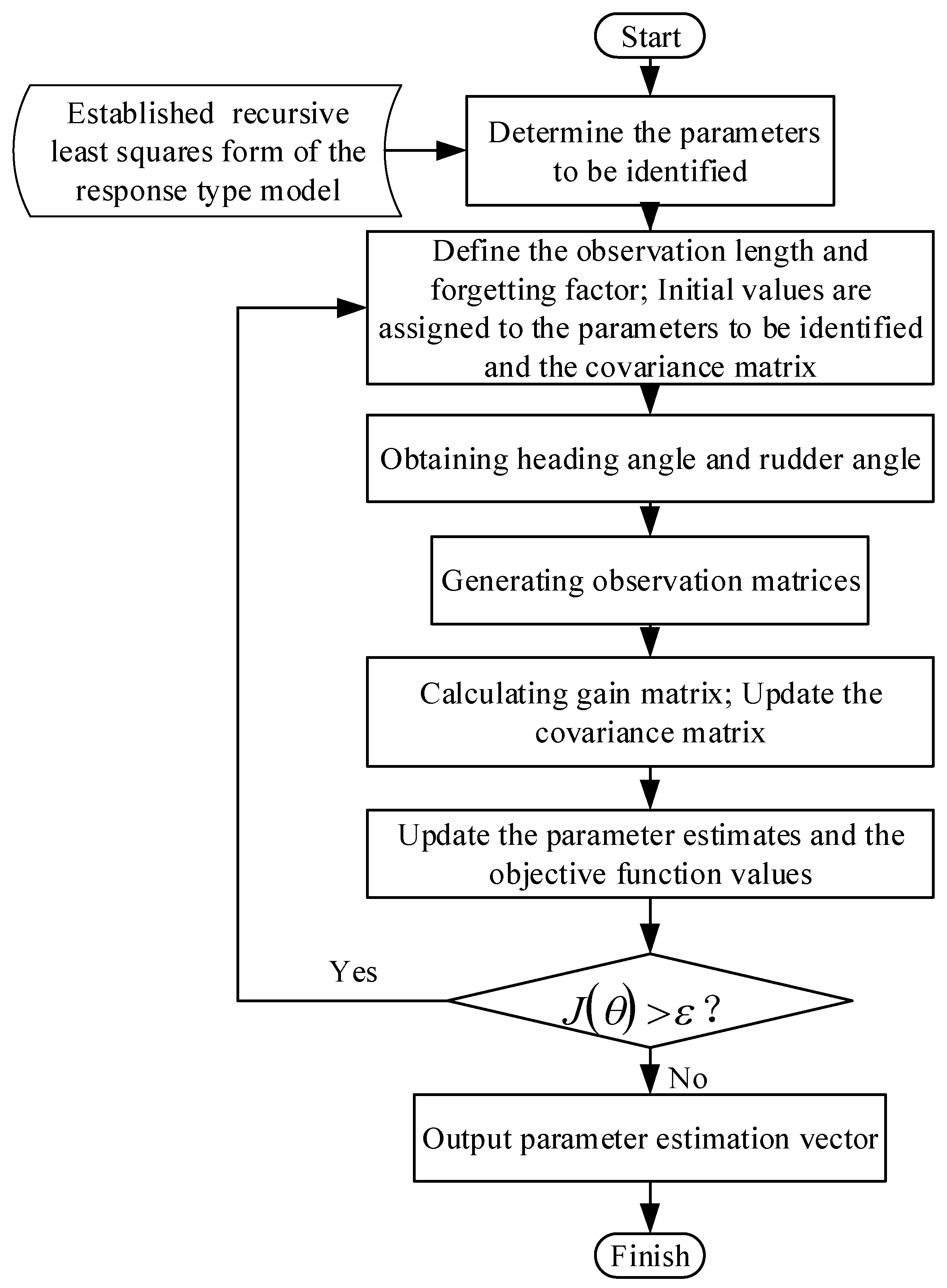
3. Parameter Identification of the Ship Maneuvering Motion Model

3.1. Recursive Least Squares Method

Least square (LS) is the most classical identification method. Its principal feature is the minimization of the root-mean-square deviation between the identification model and the real model, with the objective of maximizing the estimation of the parameters needed to be identified. It is a typical empirical risk minimization algorithm. The fundamental structure of the algorithm is as follows:

$$\mathit{Y}=\mathit{X}\mathbf{\cdot }\mathit{\theta }\left(\mathit{X}\in R^m,\mathit{Y}\in R\right)$$

(10)

where X represents the input sample, Y is the output sample, θ is the parameter to be identified, and m is the dimension of the input sample. The fundamental principle of the least square method is to identify an estimated value for an unknown vector, with the objective of achieving a minimum residual sum of squares. As can be observed from Equation (10), the error vector and objective function are as follows:

$$\min J={\displaystyle \sum _{i=1}^m{\mathit{\epsilon }}_i^2={\mathit{\epsilon }}^T\mathit{\epsilon }}$$

(11)

The objective is to minimize the value of the objective function by identifying the partial derivative of J and setting it equal to zero, where n represents the number of sample pairs:

$${\displaystyle \frac{\partial \mathit{J}}{\partial \mathit{\theta }}}\left|{}_{\mathit{\theta }=\widehat{\mathit{\theta }}}\right.={\displaystyle \frac{\partial }{\partial \mathit{\theta }}}{\left|\left(\mathit{Y}-\mathit{X}\widehat{\mathit{\theta }}\right)\right.}^T\left(\mathit{Y}-\mathit{X}\widehat{\mathit{\theta }}\right)=-2{\mathit{X}}^{\mathit{T}}\mathit{Y}+2{\mathit{X}}^T\mathit{X}\widehat{\mathit{\theta }}=0$$

(12)

The least squares estimate derived $\widehat{\theta }$ from the aforementioned equation, which is as follows:

$$\widehat{\mathit{\theta }}={\left({\mathit{X}}^{\mathrm{T}}\mathit{X}\right)}^{-1}{\mathit{X}}^T\mathit{Y}$$

(13)

The least squares algorithm displays a high degree of adaptability and is capable of producing optimal solutions for a diverse range. Nevertheless, as the quantity of data accumulates, the increasing volume of data adversely affects the real-time performance of the algorithm. Consequently, it becomes imperative to conduct parameter estimation after collecting all the data, which may introduce significant errors in ship control. In order to achieve real-time control, researchers have made enhancements to the least squares algorithm by proposing the recursive least squares algorithm, whose derivation steps are outlined below.

Rewrite Equation (10) as:

$$\mathit{y}\left(k\right)=\mathit{H}\left(k\right)\widehat{\mathit{\theta }}\left(k\right)$$

(14)

When the kth observation is made, the least squares estimate is:

$$\widehat{\mathit{\theta }}\left(k\right)={\left[{\mathit{H}}^T\left(k\right)\mathit{H}\left(k\right)\right]}^{-1}{\mathit{H}}^T\left(k\right)\mathit{y}\left(k\right)$$

(15)

Similarly, for k+1th observations, the least squares estimate is:

$$\widehat{\mathit{\theta }}\left(k+1\right)={\left[{\mathit{H}}^T\left(k+1\right)\mathit{H}\left(k+1\right)\right]}^{-1}{\mathit{H}}^T\left(k+1\right)\mathit{y}\left(k+1\right)$$

(16)

In Equation (16):

$$\mathit{H}\left(k+1\right)=\left[\begin{array}{c}\mathit{H}\left(k\right)\\ {\mathit{h}}^T\left(k+1\right)\end{array}\right],\mathit{y}\left(k+1\right)=\left[\begin{array}{c}\mathit{y}\left(k\right)\\ \mathit{y}\left(k+1\right)\end{array}\right]$$

(17)

Substitute Equation (17) into Equation (16) to obtain Equation (18):

$${\mathit{H}}^T\left(k+1\right)\mathit{H}\left(k+1\right)={\left[{\mathit{H}}^T\left(k\right)\mathit{H}\left(k\right)\right]}^{-1}+{\mathit{h}}^T\left(k+1\right)\mathit{h}\left(k+1\right)$$

(18)

Define the covariance matrix:

$$\left\{\begin{array}{l}\mathit{P}\left(k\right)={\left[{\mathit{H}}^T\left(k\right)\mathit{H}\left(k\right)\right]}^{-1}\\ \mathit{P}\left(k+1\right)={\left[{\mathit{H}}^T\left(k+1\right)\mathit{H}\left(k+1\right)\right]}^{-1}\end{array}\right.$$

(19)

The properties of the inverse transformation can be determined by employing matrix operations, which ultimately yield the derivation of Equation (20):

$$\begin{array}{l}\mathit{P}\left(k+1\right)={\left[{\mathit{H}}^T\left(k+1\right)\mathit{H}\left(k+1\right)\right]}^{-1}={\left[{\mathit{P}}^{-1}\left(k\right)+\mathit{h}\left(k+1\right){\mathit{h}}^T\left(k+1\right)\right]}^{-1}=\\ \left[\mathit{I}-\mathit{K}\left(k+1\right){\mathit{h}}^T\left(k+1\right)\right]\mathit{P}\left(k\right)\end{array}$$

(20)

Subsequently, the parameter matrix is derived as follows:

$$\begin{array}{l}\widehat{\mathit{\theta }}\left(k+1\right)=\mathit{P}\left(k+1\right){\mathit{H}}^T\left(k+1\right)\mathit{y}\left(k+1\right)=\mathit{P}\left(k+1\right)\left[\begin{array}{cc}{\mathit{H}}^T\left(k\right)& \mathit{h}\left(k+1\right)\end{array}\right]\left[\begin{array}{c}\mathit{y}\left(k\right)\\ \mathit{y}\left(k+1\right)\end{array}\right]\\ \hspace{1em}\hspace{0.5em}\hspace{1em}\hspace{1em}=\mathit{P}\left(k+1\right)\left[{\mathit{H}}^T\left(k\right)\mathit{y}\left(k\right)+h\left(k+1\right)\mathit{y}\left(k+1\right)\right]\\ \hspace{1em}\hspace{0.5em}\hspace{1em}\hspace{1em}=\widehat{\mathit{\theta }}\left(k\right)+\mathit{K}\left(k+1\right)\left[\mathit{y}\left(k+1\right)-{\mathit{h}}^T\left(k+1\right)\widehat{\mathit{\theta }}\left(k\right)\right]\end{array}$$

(21)

where K(k + 1) represents the gain matrix, $\widehat{\mathit{\theta }}\left(k\right)$ and $\widehat{\mathit{\theta }}\left(k+1\right)$ are the parameter estimation matrices at the kth and k+1th, respectively, and P(k+1) is the covariance matrix.

Once the requisite calculations have been completed, the formula for the recursive least squares algorithm can be expressed as follows:

$$\left\{\begin{array}{l}\widehat{\mathit{\theta }}\left(k+1\right)=\widehat{\mathit{\theta }}\left(k\right)+\mathit{K}\left(k+1\right)\left[\mathit{y}\left(k+1\right)-{\mathit{h}}^T\left(k+1\right)\widehat{\mathit{\theta }}\left(k\right)\right]\\ \mathit{K}\left(k+1\right)={\displaystyle \frac{\mathit{P}\left(k\right)\mathit{h}\left(k+1\right)}{1+{\mathit{h}}^T\left(k+1\right)\mathit{P}\left(k\right)\mathit{h}\left(k+1\right)}}\\ \mathit{P}\left(k+1\right)=\left[\mathbf{I}-\mathit{K}\left(k+1\right){\mathit{h}}^T\left(k+1\right)\right]\mathit{P}\left(k\right)\end{array}\right.$$

(22)

3.2. Recursive Least Square Method with Forgetting Factor

In comparison to the conventional least square method, the recursive least square method presents a substantial advantage in terms of enabling online parameter identification. However, the continuous update of data results in an increase in matrix elements, which in turn causes the inverse matrix to approach zero at a gradual rate. Consequently, the rate of model update speed slows down progressively, potentially reaching a point where it is unable to continue running due to data saturation. In essence, the excessive accumulation of past information renders the current data insignificant in comparison to their predecessors, resulting in an inability to discern any impact. To address the issue of data saturation, a forgetting factor is introduced.

The recursive least squares method with forgetting factor serves to augment the weight of new data, strengthen the influence of new data, reinforce the impact of new data on the model, diminish the weight of old data, and enhance the algorithm by conferring disparate weights upon disparate data. The forgetting factor is represented by λ and an exponential function weight is employed to determine the weighting. In this instance, the performance index of the algorithm is as follows:

$$J={\displaystyle \sum _{k=1}^L{\lambda }^{L-k}{\left[\mathit{y}\left(k\right)-\mathit{h}\left(k\right)\widehat{\mathit{\theta }}\left(k\right)\right]}^2}$$

(23)

In the case where the forgetting factor is typically assumed to be within the range of 0.98 to 0.995 [19], the most recent data are given a weighting of 1 while the data from the preceding n sampling periods are assigned a weighting of λn. Following the introduction of the forgetting factor, the iterative calculation formula is revised as follows:

$$\left\{\begin{array}{l}\widehat{\mathit{\theta }}\left(k\right)=\widehat{\mathit{\theta }}\left(k-1\right)+\mathit{K}\left(k\right)\left[\mathit{y}\left(k\right)-{\mathit{h}}^T\left(k\right)\widehat{\mathit{\theta }}\left(k-1\right)\right]\\ \mathit{K}\left(k\right)={\displaystyle \frac{\mathit{P}\left(k-1\right)\mathit{h}\left(k\right)}{1+{\mathit{h}}^T\left(k\right)\mathit{P}\left(k-1\right)\mathit{h}\left(k\right)}}\\ \mathit{P}\left(k\right)={\displaystyle \frac{1}{\lambda }}\left[I-K\left(k\right){\mathit{h}}^T\left(k\right)\right]\mathit{P}\left(k-1\right)\end{array}\right.$$

(24)

The recursive least squares method with a forgetting factor is an effective approach for identifying the parameters of a model. This method allows the system to focus more on the current data while also accounting for previous data in a meaningful way. The performance of the algorithm is primarily influenced by the forgetting factor. A small forgetting factor results in rapid convergence but also renders the algorithm susceptible to noise, thereby compromising the precision of parameter identification. Conversely, a large λ enhances the anti-noise performance of the algorithm but impedes convergence. Consequently, the value of λ plays a pivotal role in the algorithmic performance, necessitating a trade-off between convergence speed and noise sensitivity to achieve optimal results.

3.3. Parameter Identification of Responsive Ship Motion Model

As demonstrated in the preceding section, the recursive least squares method is well-suited for discrete-time mathematical models, as evidenced by its derivation process. Consequently, the established continuous mathematical model is transformed into a discrete mathematical model and the differential is rearranged into the standard least squares form, resulting in the following expression:

$$\left\{\begin{array}{l}\mathit{y}\left(k\right)=\mathit{\phi }\left(k\right)\widehat{\mathit{\theta }}\left(k\right)\\ \mathit{\phi }\left(k\right)=\left[\begin{array}{cc}r\left(k\right)& \delta \left(k\right)\end{array}\right]\\ \widehat{\mathit{\theta }}\left(k\right)={\left[a_1 b_1\right]}^{\mathrm{T}}\end{array}\right.$$

(25)

where φ(k) is the input vector, including the heading angular velocity r(k) and rudder angle δ(k) at time k, $\widehat{\mathit{\theta }}\left(k\right)$ is the parameter vector to be identified. However, considering that the heading angular velocity is difficult to measure and the accuracy is poor in the real ship test or ship model test, the heading angle is usually measured by compass. Therefore, it is necessary to difference the course angle in the response model:

$$\mathit{y}\left(k+2\right)=a\mathit{y}\left(k+1\right)+b\mathit{u}\left(k\right)$$

(26)

where $\mathit{y}\left(k+2\right)=\mathit{\psi }\left(k+2\right)-\mathit{\psi }\left(k+1\right)$, $\mathit{u}\left(k\right)=\delta \left(k\right)$, and the transformation relationship between a₁, b₁, and K, T is as follows:

$$\left\{\begin{array}{l}T={\displaystyle \frac{\Delta t}{1-a}}\\ K={\displaystyle \frac{b}{\left(1-a\right)\Delta t}}\end{array}\right.$$

(27)

where $\Delta t$ is the sampling period, which is taken as 1 s in this paper, and the identification formula is as follows:

$$\left\{\begin{array}{l}\widehat{\mathit{\theta }}\left(k\right)=\widehat{\mathit{\theta }}\left(k-1\right)+\mathit{K}\left(k\right)\left[\mathit{\psi }\left(k\right)-{\mathit{\phi }}^T\left(k\right)\widehat{\mathit{\theta }}\left(k-1\right)\right]\\ \mathit{K}\left(k\right)={\displaystyle \frac{\mathit{P}\left(k-1\right)\mathit{\phi }\left(k\right)}{1+{\mathit{\phi }}^T\left(k\right)\mathit{P}\left(k-1\right)\mathit{\phi }\left(k\right)}}\\ \mathit{P}\left(k\right)={\displaystyle \frac{1}{\lambda }}\left[\mathit{I}-\mathit{\phi }\left(k\right){\mathit{\phi }}^T\left(k\right)\right]\mathit{P}\left(k-1\right)\end{array}\right.$$

(28)

The complete iterative flow chart of parameter identification for the responsive motion mathematical model is shown in Figure 3 as follows:

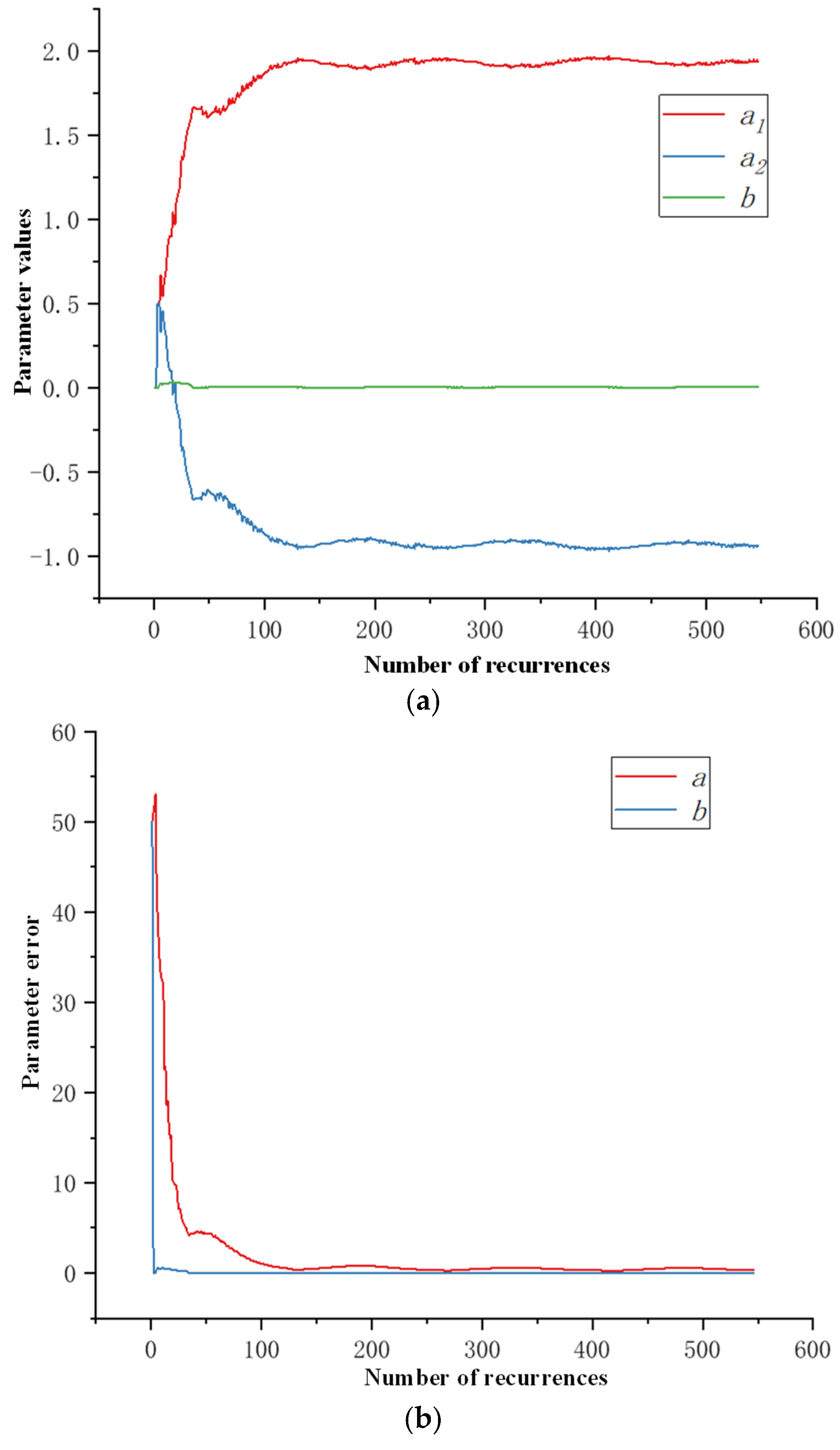
3.4. Analysis of Identification Algorithm Based on Ship Maneuvering Simulator

In order to ascertain the veracity of the recursive least squares method with forgetting factor, the ship in the ship maneuvering simulator was employed as the test ship to obtain the response data. Initially, the ship was operated on the platform for maneuvers, with the heading angle and rudder angle information recorded by the sensor equipment, and then integrated into NMEA-0183 format for transmission through TCP. Finally, the data were decoded for the parameter identification algorithm to call. The ship shape and some ship parameters are shown in

Table 1. Parameters of the ship.

Parameter	Value
Displacement (t)	69,580
Length (m)	230
Breadth (m)	32
Bow draft (m)	12
Stern draft (m)	12
Height of eye (m)	22

. In the presence of wind, wave, and current interference, two sets of maneuverability index identification tests were conducted at varying speeds, with the resulting identification data employed for course prediction.

Based on the data of the ship maneuvering simulator, different forgetting factors were used to identify the parameters of the responsive model and the influence of different forgetting factors on parameter identification was compared. The process of parameter identification is shown in the following figures.

Combining Figure 4, Figure 5, and

Table 2. Error of identification with different forgetting factors.

Value of the Forgetting Factor	The Error Value of a	The Error Value of a
0.99	0.117843	0.004218
0.98	0.303138	0.015827

reveals that the convergence patterns of all parameters show a remarkable similarity: as the number of recursions increases, they begin to stabilize around the 150th recurrence before converging to a fixed value. In the last recursion, a₁ = 1.9375, a₂ = −0.9375, and b = 0.00467 in Figure 5 while a₁ = 1.9601, a₂ = −0.9601, and b = 0.00235 in Figure 6. Here, a₁ and a₂ represent newly introduced parameters in the differential transformation of the response model whose sum is equal to one. By comparing the identification curves of two forgetting factors, it can be observed that smaller forgetting factors result in higher noise sensitivity and better system tracking capability at the expense of increased steady-state error. Considering that most actual ship maneuvering involves external disturbances, a forgetting factor of 0.98 was selected. After selecting the appropriate forgetting factor, the recursive least squares method with forgetting factor and the conventional least squares method were used to identify K and T, respectively, and the 20°/20° Z-shape test was carried out according to the identification results. The test results are shown in Figure 6.

In the above figure, the blue curve is the predicted course change curve and the red curve is the actual output course change curve of the ship maneuvering simulator. It can be seen from the figure that in both the ordinary least squares method and the recursive least squares method with forgetting factor, the predicted course angle through identification is in good agreement with the actual output value, which has a certain accuracy. The maximum prediction error of the recursive least squares method with forgetting factor is about 3° and the maximum prediction error of the ordinary least squares method is about 5°. The prediction results of the former are more consistent. Therefore, the K and T values identified by the recursive least squares method with forgetting factor are practical and effective and have certain advantages compared with the traditional least squares method.

The parameters K and T were calculated or identified using Equation (8) and FFRLS, respectively, and compared with the actual K and T values provided by the ship maneuvering simulator. The results are shown in

Table 3. Parameter calculation/identification comparison.

Parameter	True Value	Equation (8)	FFRLS
K	0.13	0.18	0.157
T	180	198	192

.

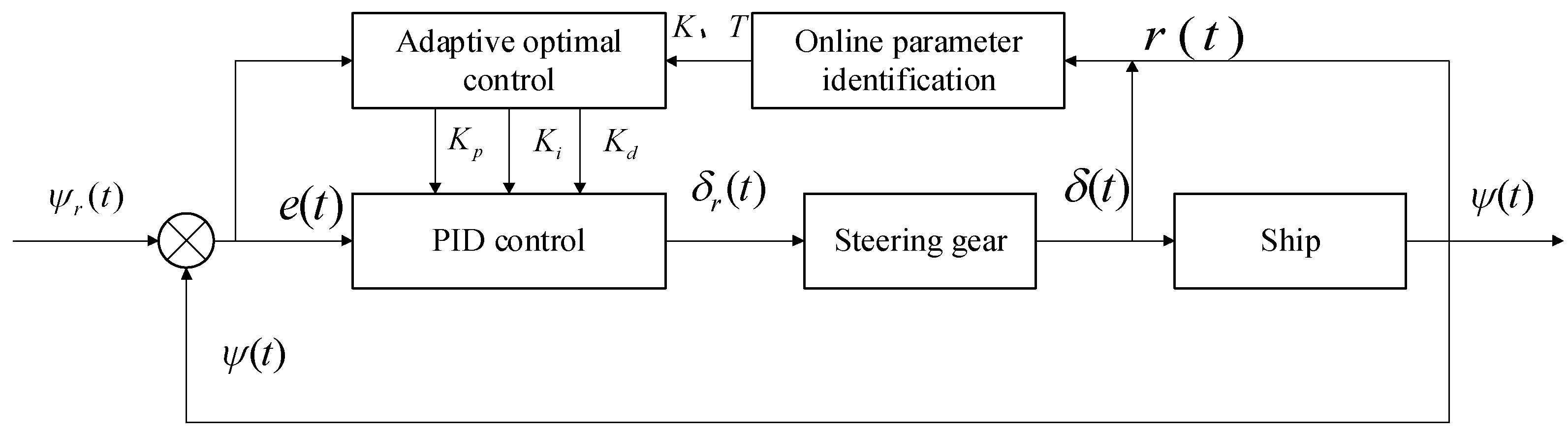
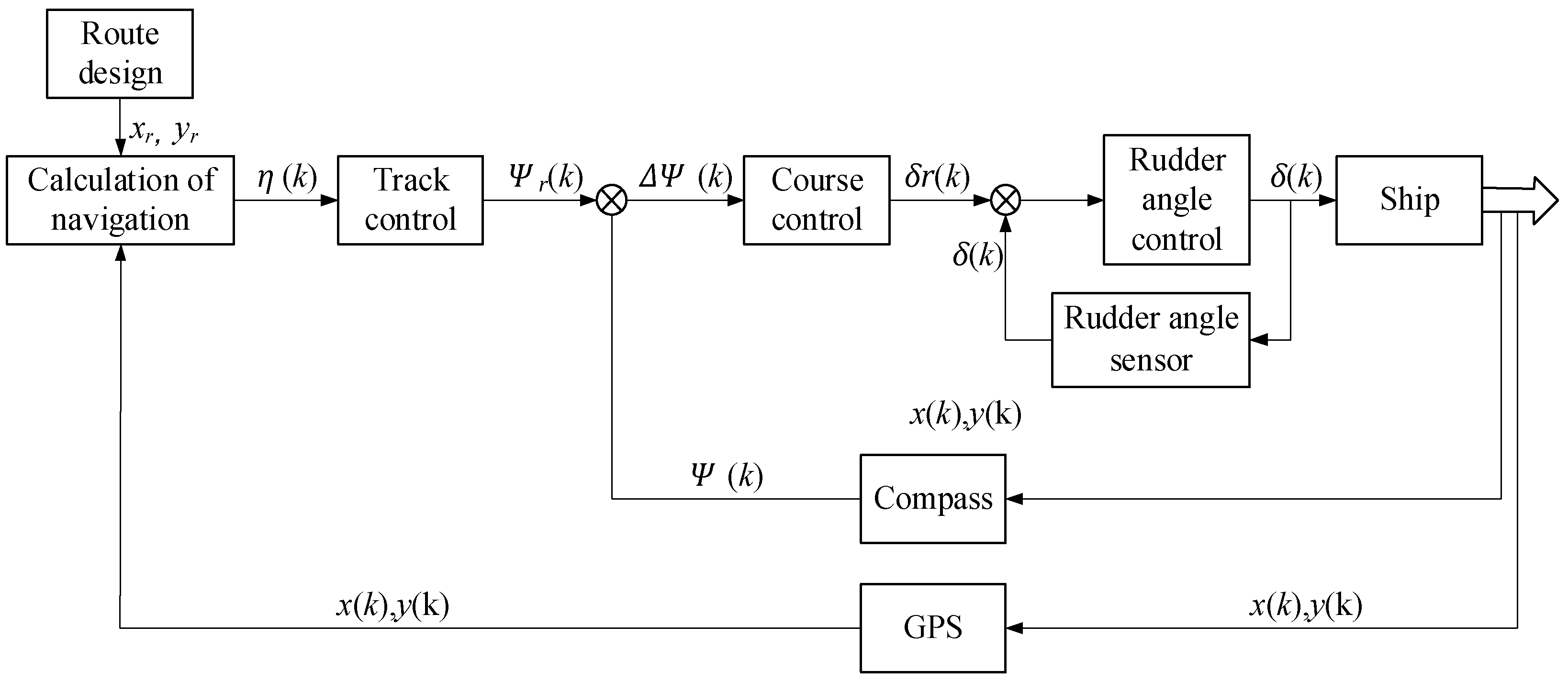
4. Ship Course and Track Control Method

4.1. PID Course Control Method Based on Optimal Control Theory

The three parameters, K_p, K_i, and K_d, of the traditional PID course autopilot are mostly determined by the ship’s pilots or related technicians based on experience or repeated trials. Generally, they are a set of fixed values, which cannot be adjusted adaptively according to the changing motion state of the ship and other factors so the autopilot cannot achieve the best control effect in many cases. Considering the quadratic optimal control method [16], an algorithm that can obtain the OP-PID parameters is designed based on the original PID control research to improve the control effect of PID.

According to the Nomoto equation of Equation (9), the state equation of ship steering can be obtained as follows:

$$\left[\begin{array}{c}\dot{\psi }\\ \ddot{\psi }\end{array}\right]=\mathit{A}\left[\begin{array}{c}\psi \\ \dot{\psi }\end{array}\right]+\mathit{B}\delta$$

(29)

The output equation is as follows:

$$\psi =\mathit{C}\left[\begin{array}{c}\psi \\ \dot{\psi }\end{array}\right]$$

(30)

The matrix in the above equation is as follows:

$$\mathit{A}=\left[\begin{array}{cc}0& 1\\ 0& -{\displaystyle \frac{1}{T}}\end{array}\right],\mathit{B}=\left[\begin{array}{c}0\\ {\displaystyle \frac{K}{T}}\end{array}\right],\mathit{C}=\left[\begin{array}{cc}1& 0\end{array}\right]$$

(31)

When ship sailing, it is necessary to reduce energy consumption as much as possible while maintaining the accuracy of the heading course. Frequent steering can accurately control the course but it will also increase energy consumption and reduce the speed. In order to balance them, the quadratic performance index function is used for optimization [20]. The energy consumption and course deviation are taken as variables and the function value of Equation (32) is minimized by adjusting the control parameters:

$$J={\displaystyle {\int }_0^t\left[{\left(\Delta \psi \right)}^2+m{\delta }^2\right]}dt$$

(32)

where m is the weighting coefficient, whose value changes according to environmental conditions, generally ranging from 0.1 to 10 (its specific values are given in

Table 4. The value of m corresponds to the wind speed table.

Wind Speed (m/s)	[0,5]	(5,10]	(10,14]	(14,17]	(17,20]	(20,30]	(30,+∞)
m	0.1	4.0	8.0	8.5	9.0	9.5	10.0

), and J is the comprehensive evaluation index.

Based on the above constraints, the corresponding PID parameters can be obtained, as shown in Equation (33). The relevant mathematical principle and derivation process have been elaborated in detail in the relevant reference [20] and will not be expanded here:

$$\left\{\begin{array}{l}{K}_p=\frac{1}{\sqrt{\lambda }}\\ K_i=\frac{1}{10}\sqrt{\frac{K}{T{\lambda }^{\frac{3}{2}}}}\\ K_d=\frac{1}{K}\left(\sqrt{1+\frac{2KT}{\sqrt{\lambda }}}-1\right)\end{array}\right.$$

(33)

Compared with the traditional empirical setting method, the PID parameters obtained from the above equation perform better in terms of course convergence time, rudder angle adjustment frequency, and variation amplitude. The author has carried out relevant simulation experiments, which will not be repeated here and can refer to reference [21].

4.2. Adaptive OP-PID Course Control Method

According to Equation (33), it is easy to find that the key to OP-PID parameters lies in the ship’s maneuverability indexes K and T. In previous related studies, the statistical formula of Equation (11) is mostly used to calculate them, which also has certain adaptability. In Chapter 3, based on solving the problems that conventional least squares cannot be identified online and the updating speed of recursive least squares becomes slow with time, this paper tries to use the recursive least squares method with forgetting factor to control ship motion and its structure diagram is shown in Figure 7 below:

Here, e(t) is the difference between the target course and the actual course.

The following closed-loop system stability proof is performed. K and T are constant and positive, both according to statistical formulas and online parameter identification. Figure 8 shows the parameter identification results and the curve of ship speed changing.

Given the model equation of the control system, the characteristic equation of the system shown in Equation (34) can be obtained according to Equation (5):

$$T{\sigma }^3+\left(1+K{K}_d\right){\sigma }^2+K{K}_i+K{K}_p=0$$

(34)

It can be seen from Figure 8 that K > 0 and T > 0. And because λ > 0, we can determine that K_p > 0, K_i > 0, and K_d > 0, that is, all the coefficients of the characteristic equation are positive, and the elements in the first column of Rouse’s table are positive. According to the Routh criterion, the control system is stable.

4.3. Track Control Method

Indirect track control, which is more mainstream and easy to implement at present, is adopted and its process is shown in Figure 9.

Indirect track control consists of three loops coupled to each other. The outer loop compares the position data obtained by the ship position sensor with the planned route to calculate the track deviation η(k). The target course Ψr(k) obtained by the guidance method is used as the input of the course control loop to guide the ship to sail in the direction of eliminating the track deviation. In the middle loop, the actual course Ψ(k) is compared with the target course Ψr(k), and the course error ∆Ψ(k) is calculated, which is denoted as Ψr(k) – Ψ(k) and is the input of the course controller. The command rudder angle δr(k) is calculated by the course controller and transmitted to the rudder angle control loop to control the ship to sail in the direction of reducing the course deviation.

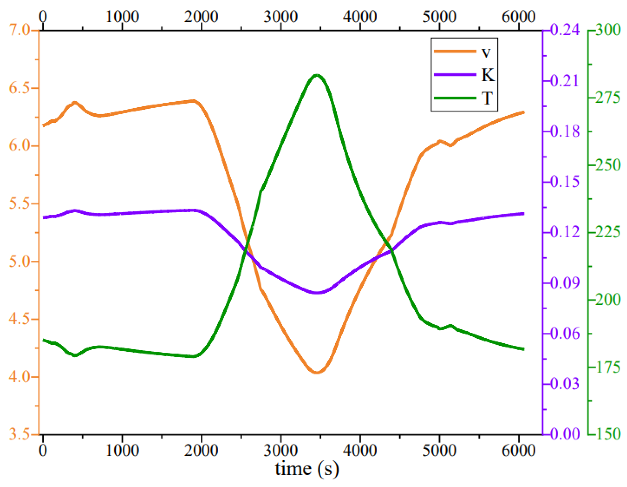
5. Simulation Experiments and Analysis

The experimental scenarios were conducted in open waters using the ship maneuvering simulator. Comparative tests were performed across multiple trials, involving different ship types and environmental disturbances. The tests compared course and track control using both OP-PID and Adaptive OP-PID controllers. The parameters for the OP-PID were obtained through the regression formula of Equations (8) and (9), while the parameters for the Adaptive OP-PID were identified online using the recursive least squares method with a forgetting factor, as introduced in Chapter 3. The Line-of-Sight (LOS) guidance method [22] was employed for route control in all cases. The key parameters for the two selected ship types are shown in

Table 5. Parameters of different ship types.

Parameter	Ship Type I	Ship Type II
Displacement (t)	69,580	8682
Length (m)	230	110
Breadth (m)	32	16.1
Bow draft (m)	12	6.4
Stern draft (m)	12	7.1
Height of eye (m)	22	12

.

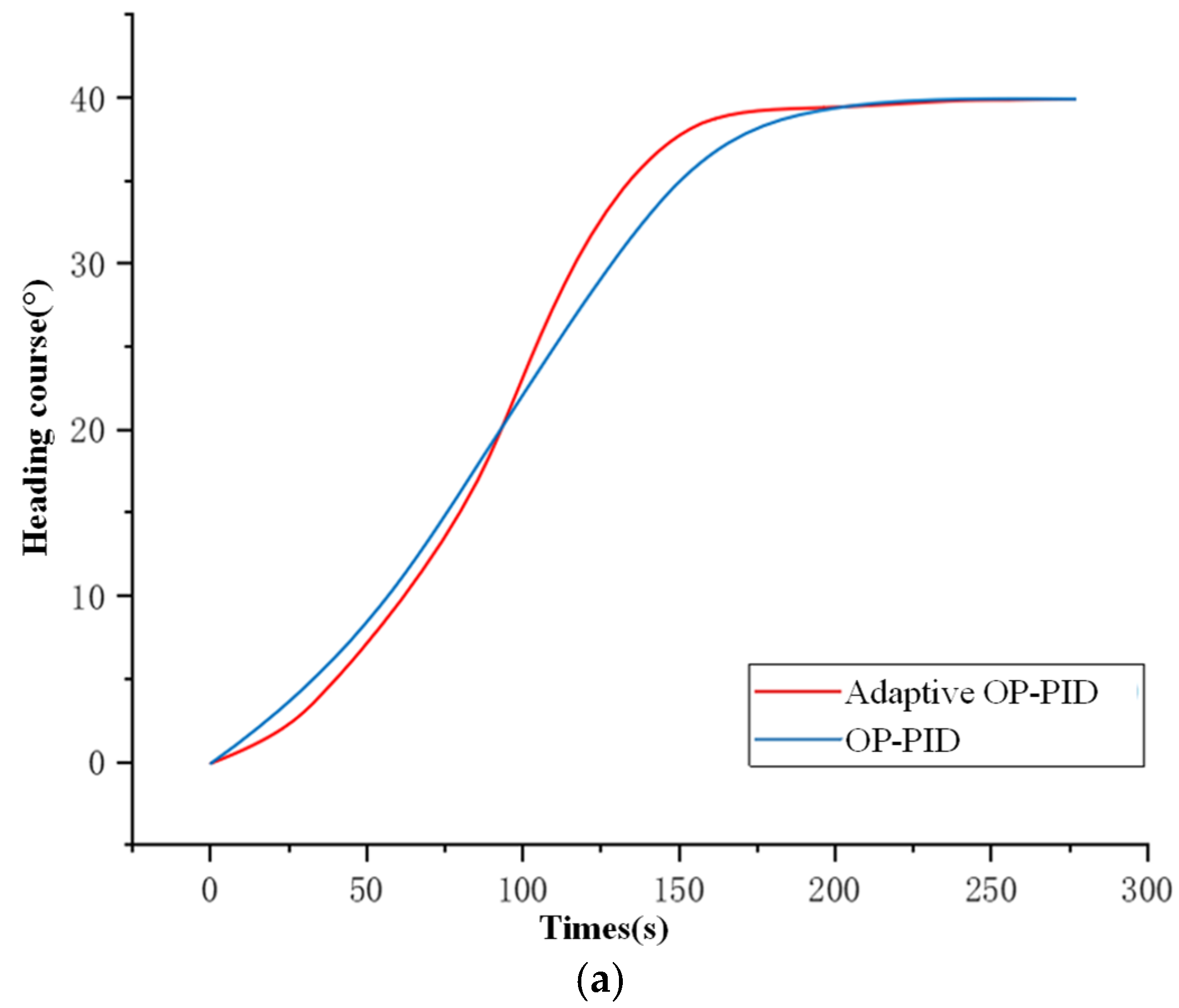
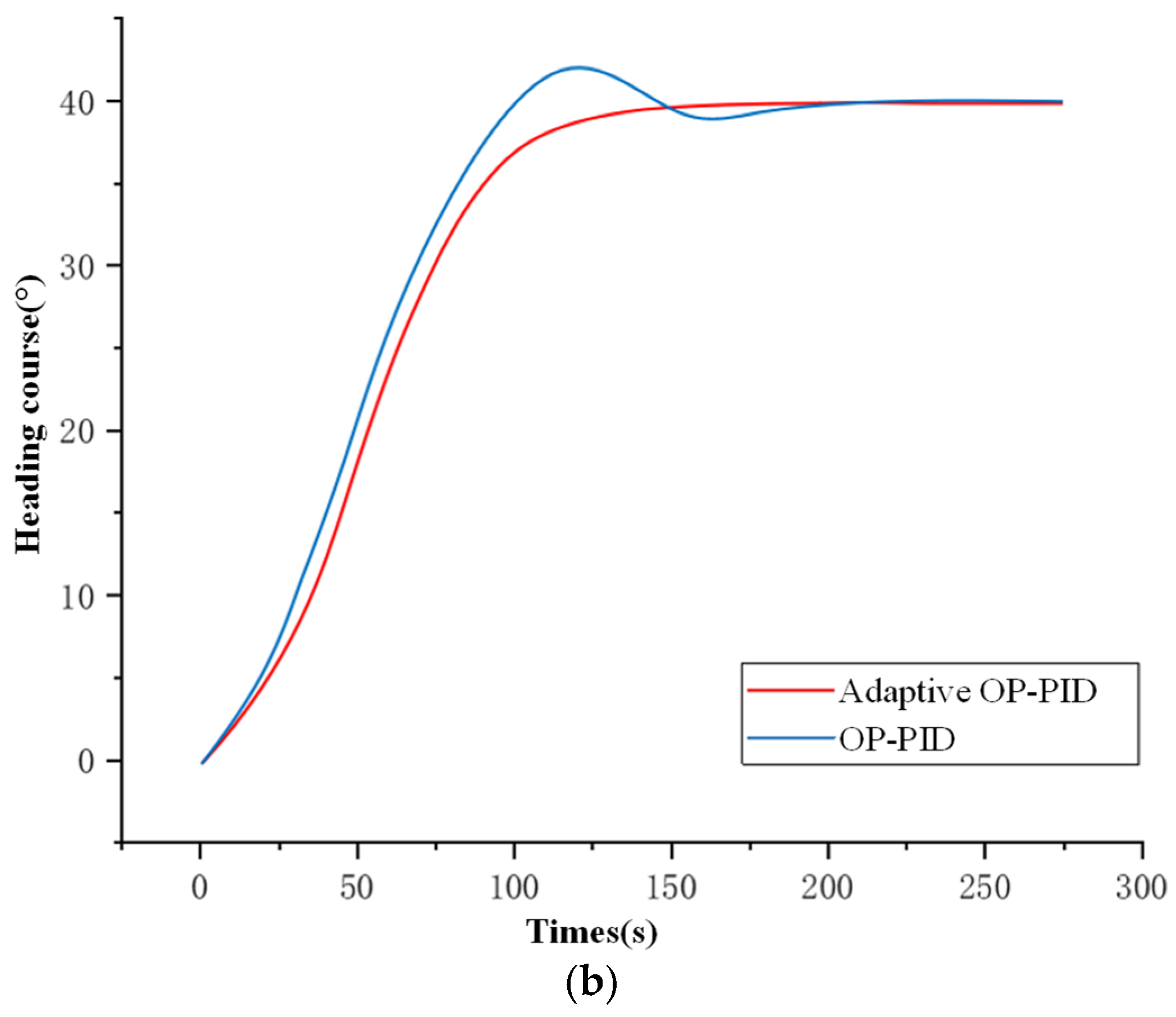
5.1. Course Control Simulation

5.1.1. Simulation of Course Control in Still Water

In calm water conditions, the initial speed of Ship Type I is set to 12 knots and slowly reduced, the initial heading course is 000, and the ship is steered from the initial course to 040 using the OP-PID and Adaptive OP-PID control methods. The experiment ends when the ship stabilizes its heading and the same experiment is repeated using Ship Type II. The ship’s course control process can be displayed on the ship maneuvering simulator ’s display interface. Figure 10 and Figure 11 show the change in the motion trajectory of Ship Type I and Ship Type II under the control of the two control methods, respectively, with the white rectangle representing the actual ship position.

It is difficult to compare the advantages and disadvantages of the control effect only by means of the motion trajectory. After exporting and processing the experimental data of the ship maneuvering simulator, the course change curve of the ship in the above test is drawn, respectively, as shown in Figure 12.

In Figure 12a, there is no overshoot in the course control test of Ship Type I by the two methods but the Adaptive OP-PID tends to be stable at about 170 s while the OP-PID tends to be stable at about 200 s. In Figure 12b, Ship Type II, controlled by the OP-PID, will continue to increase after the heading course reaches the target angle of 040, the maximum overshoot is about 3.2°, and the overshoot amplitude is about 8%. However, the Adaptive OP-PID has no obvious overshoot.

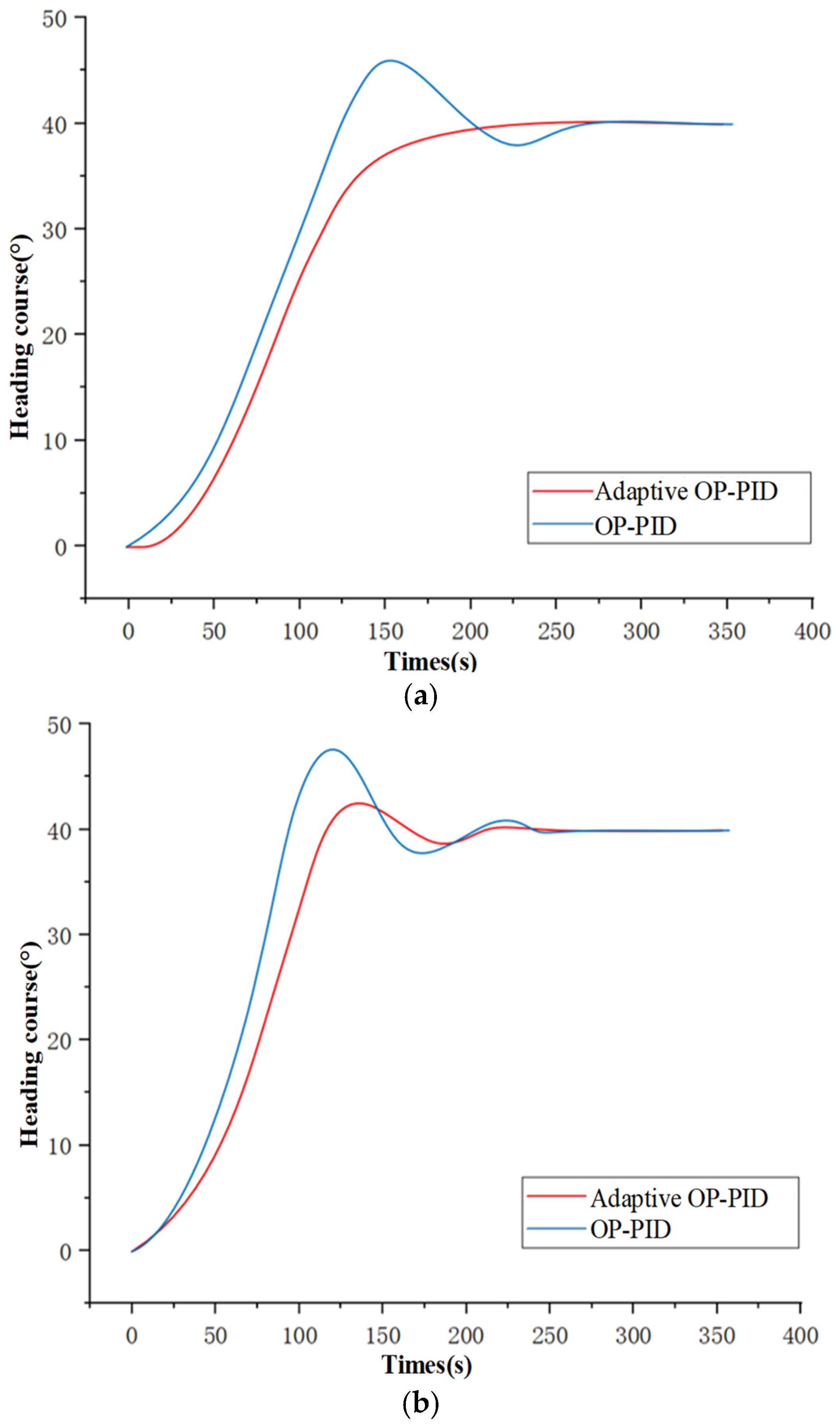
5.1.2. Simulation of Course Control Under Disturbance

Similarly, wind, wave, and current disturbance are added under the premise that other initial conditions remain unchanged, where the wind speed is 6 m/s, the current speed is 1 m/s, the wave height is 0.3 m, and the direction is 000. The motion trajectory of the ship is shown in Figure 13 and Figure 14.

Similarly, the experimental data were derived and the course change curve was plotted, as shown in Figure 15.

In Figure 15a, the Adaptive OP-PID control does not exhibit overshoot in a course under external disturbance while the OP-PID control has an overshoot of about 5.5° and an overshoot amplitude of 13.75%. In Figure 15b, both methods exhibit some degree of overshoot, with the maximum overshoot of the OP-PID being about 7.5° with an overshoot amplitude of 18.75% while the maximum overshoot of the Adaptive OP-PID is about 2.5° with an overshoot amplitude of 6.25%.

Comparing the heading course control experiments of multiple groups, it can be concluded that the Adaptive OP-PID can adapt to different ship types and external environments and its performance in course control stability and convergence time is better than that of the OP-PID.

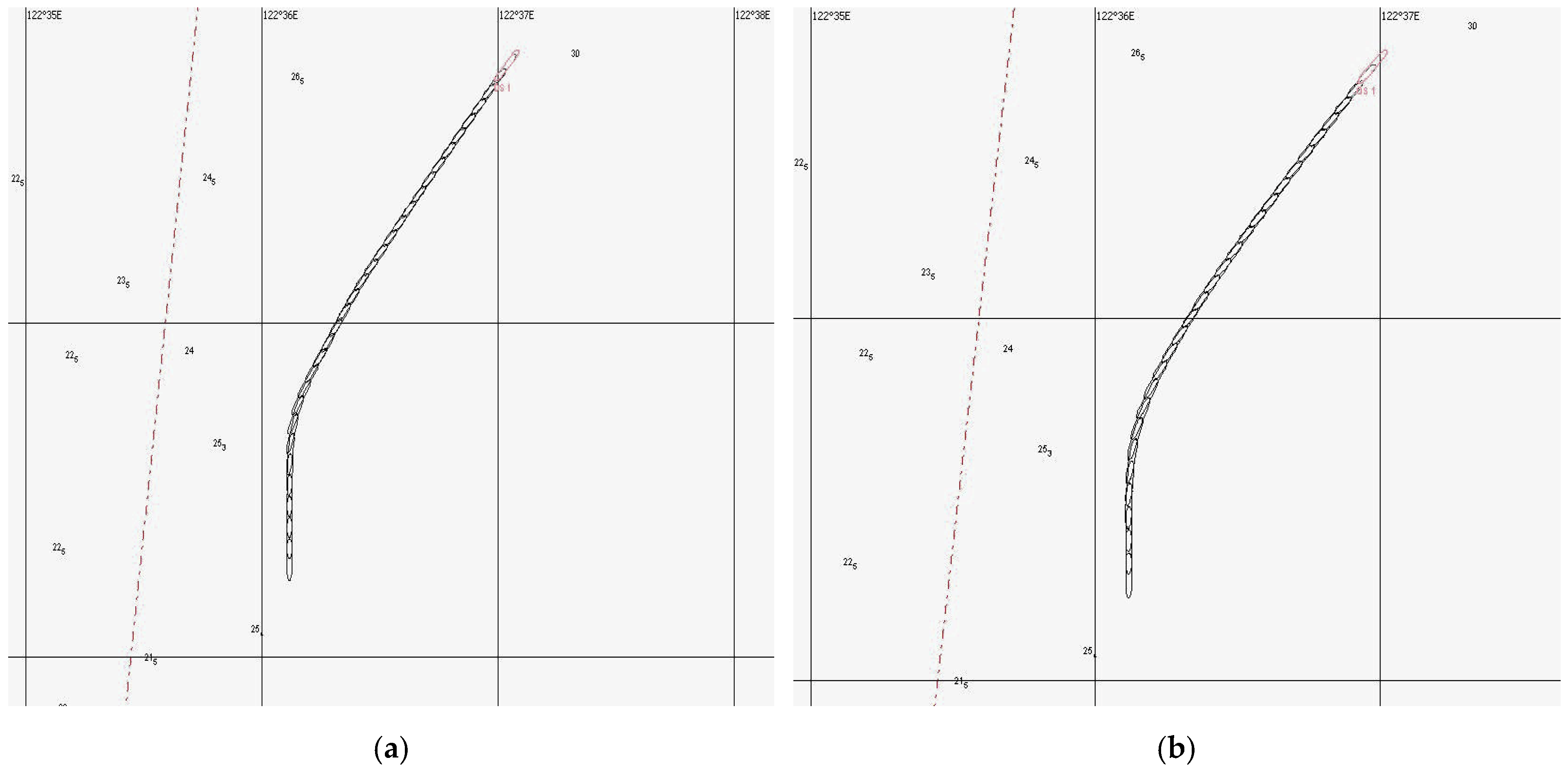
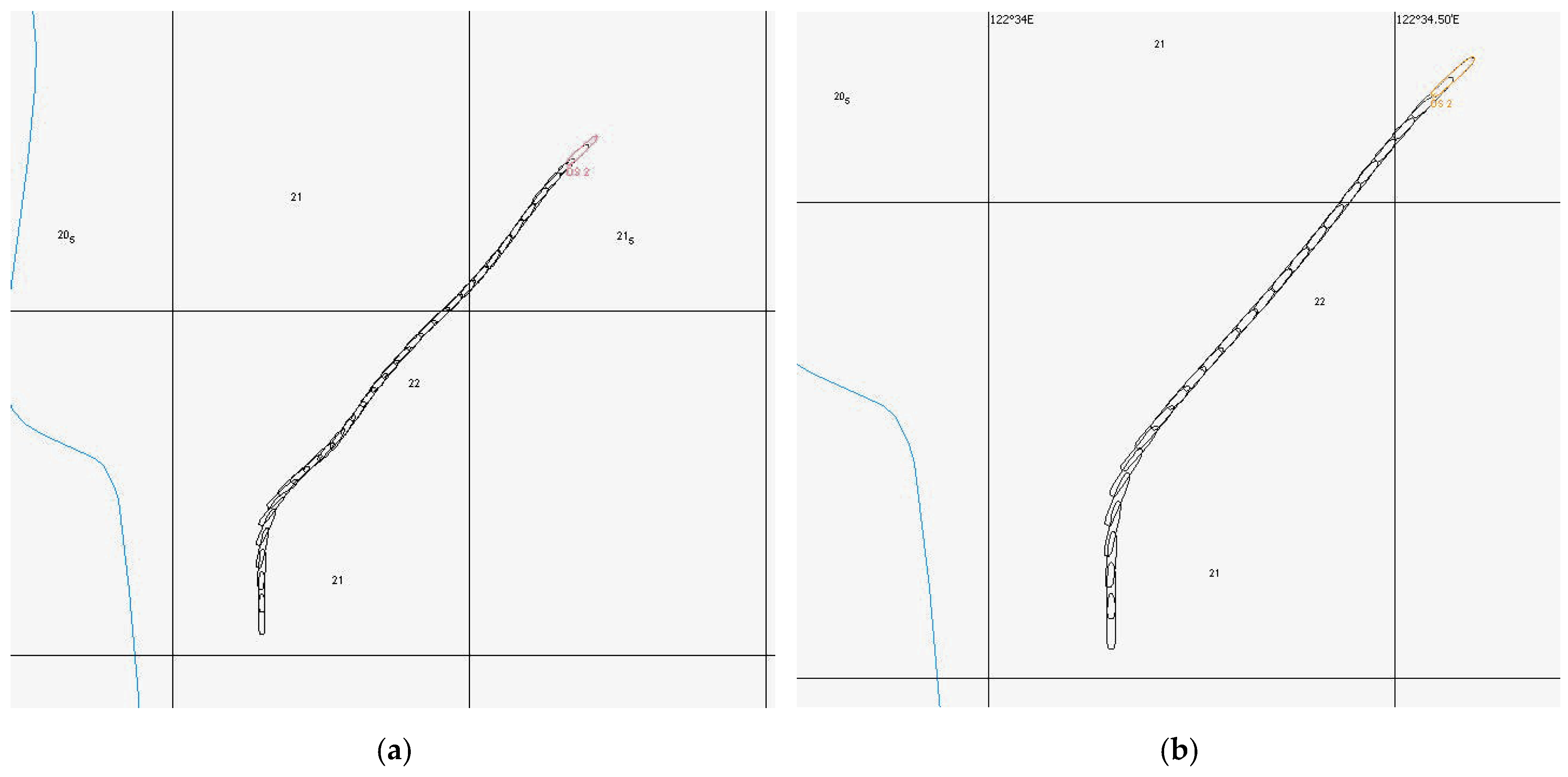
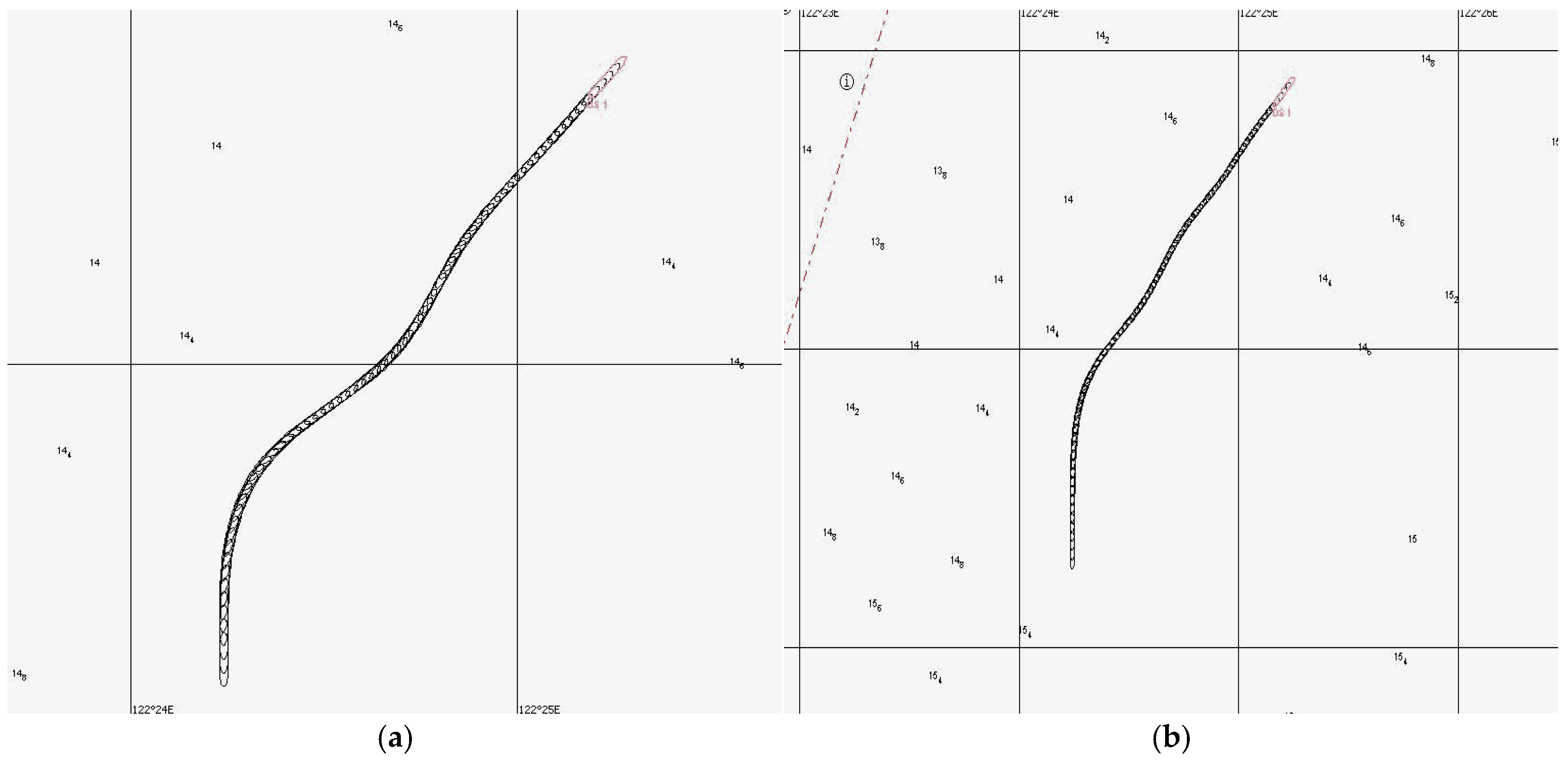
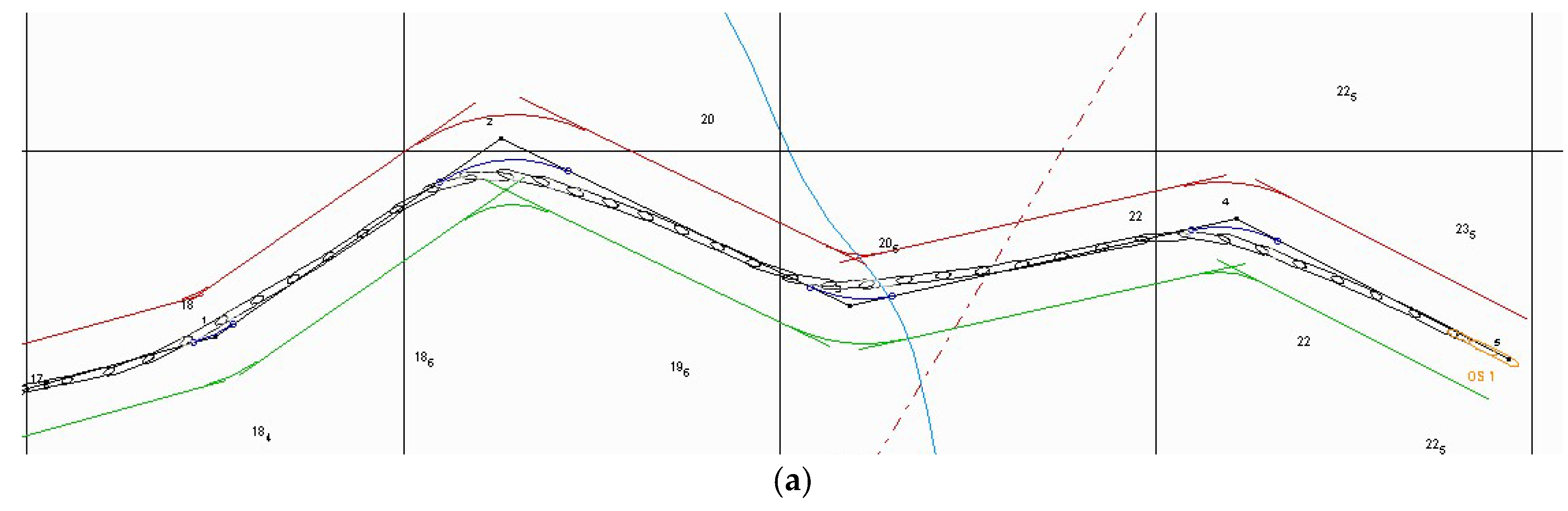
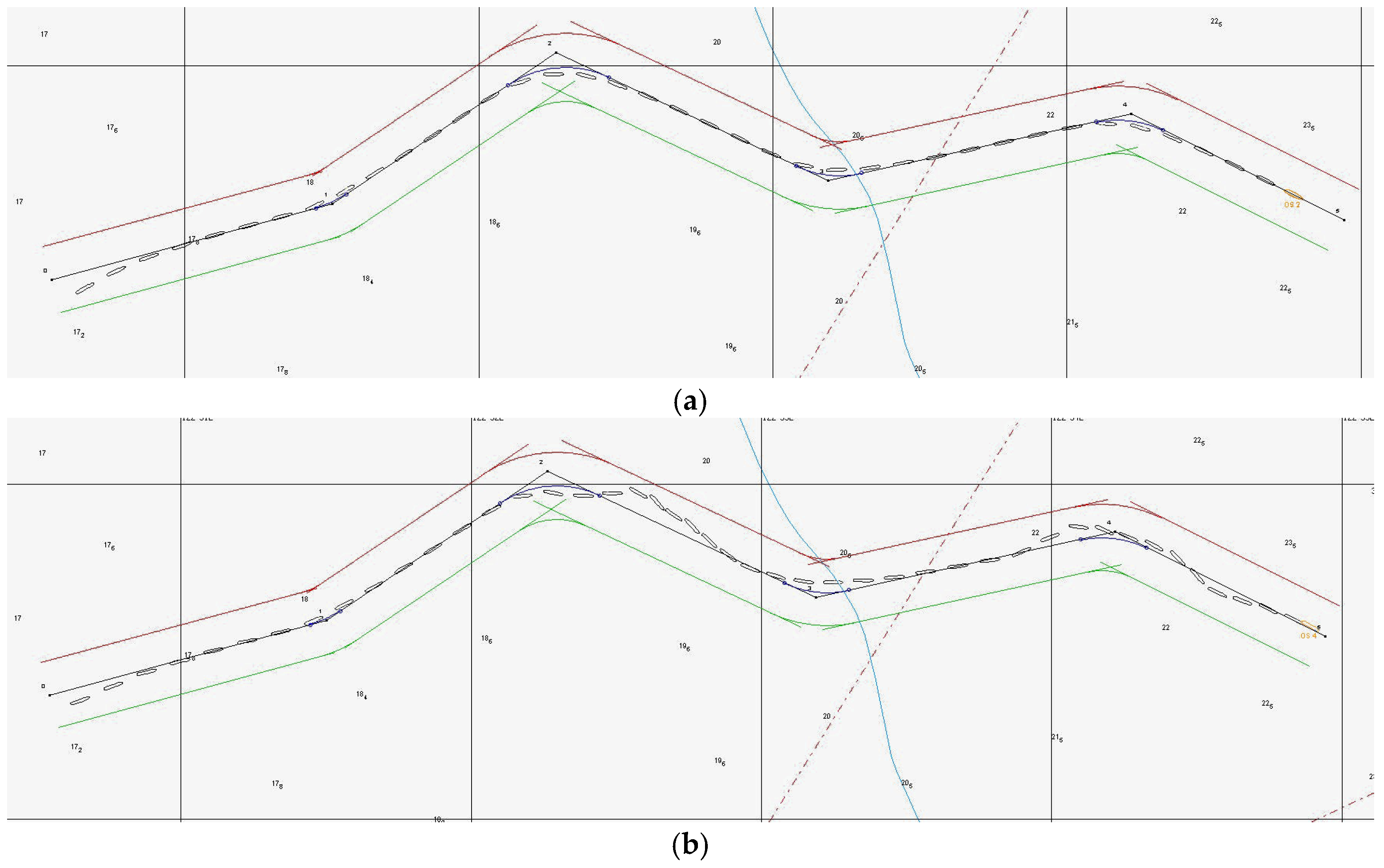
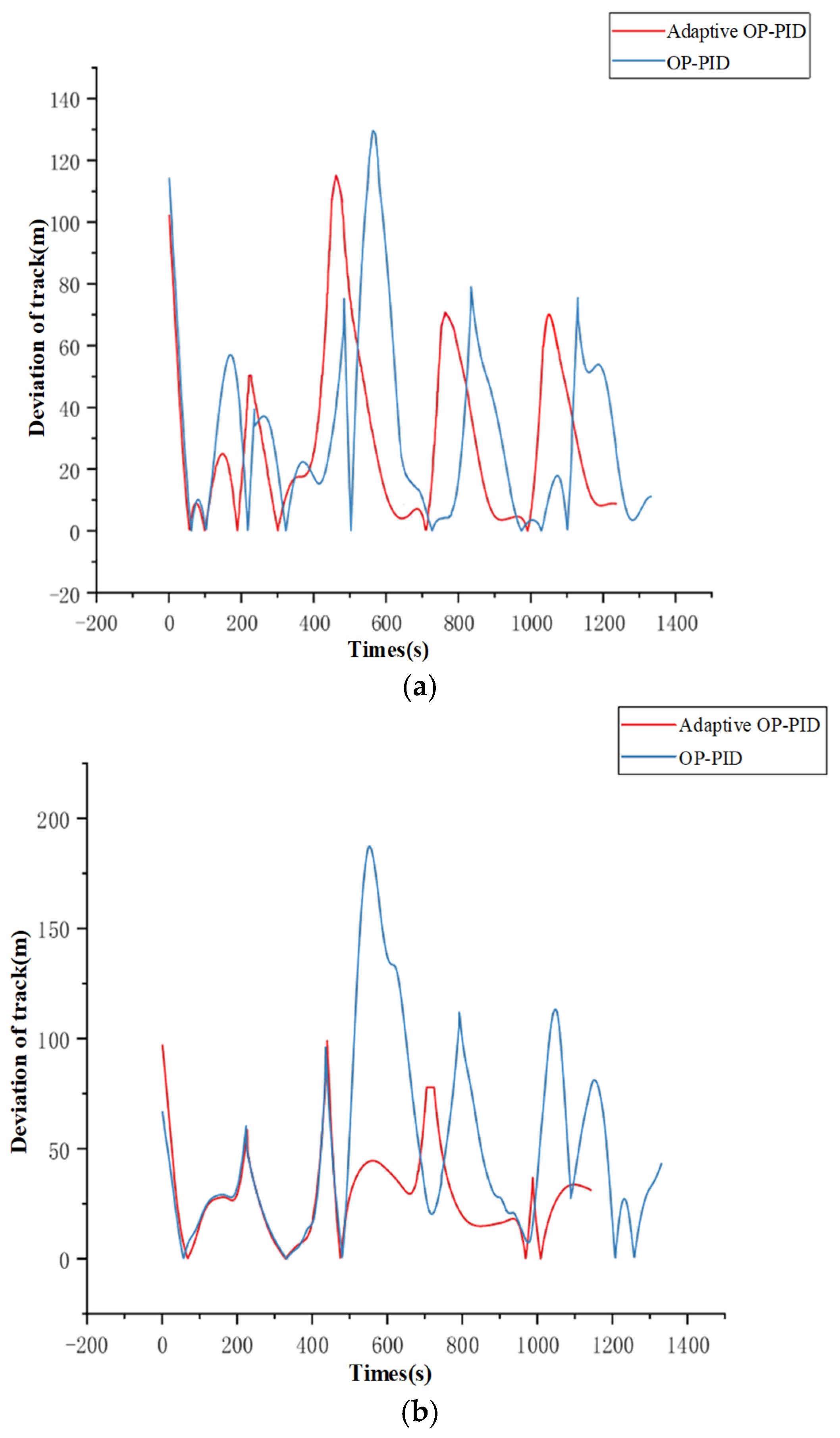
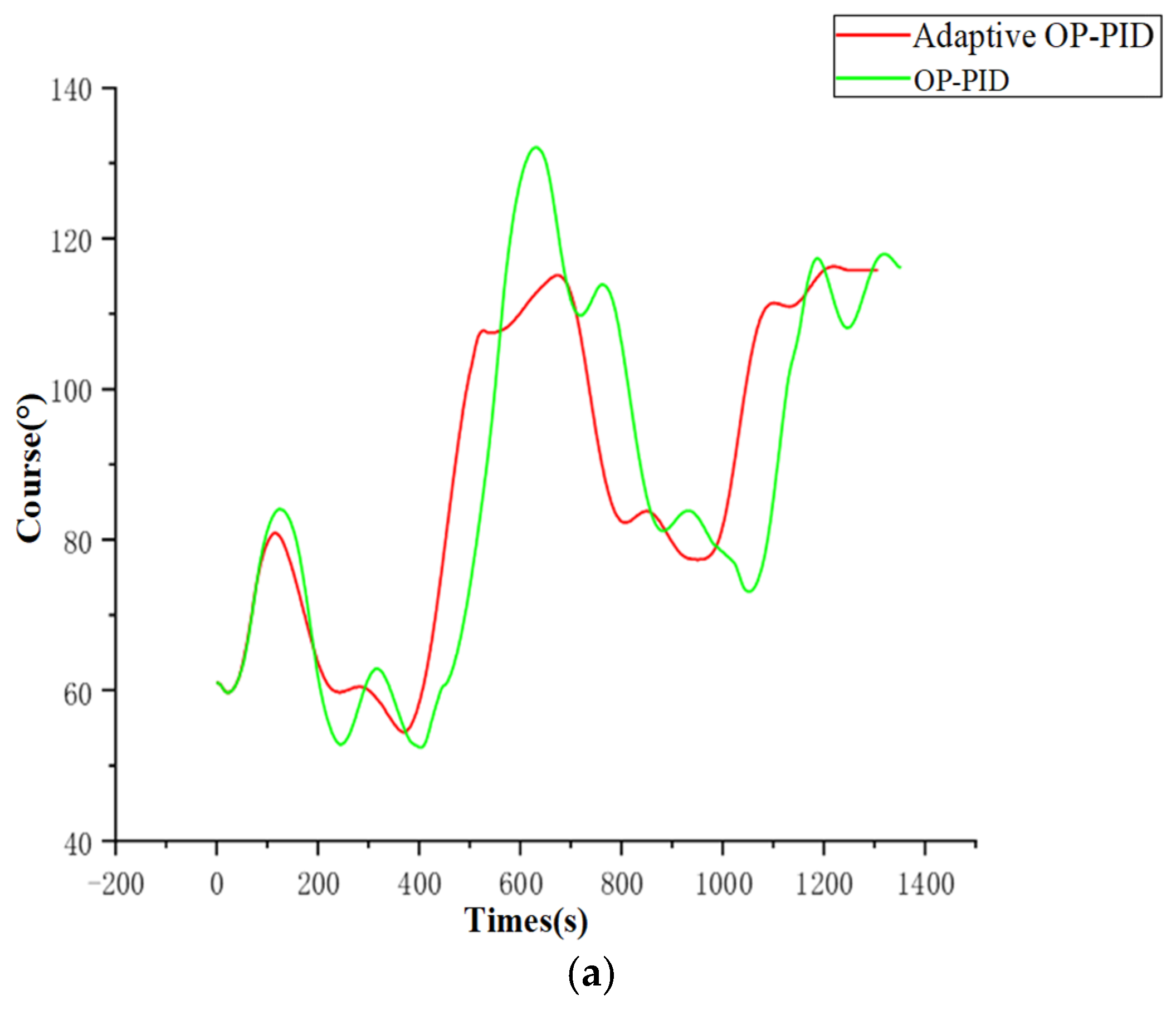
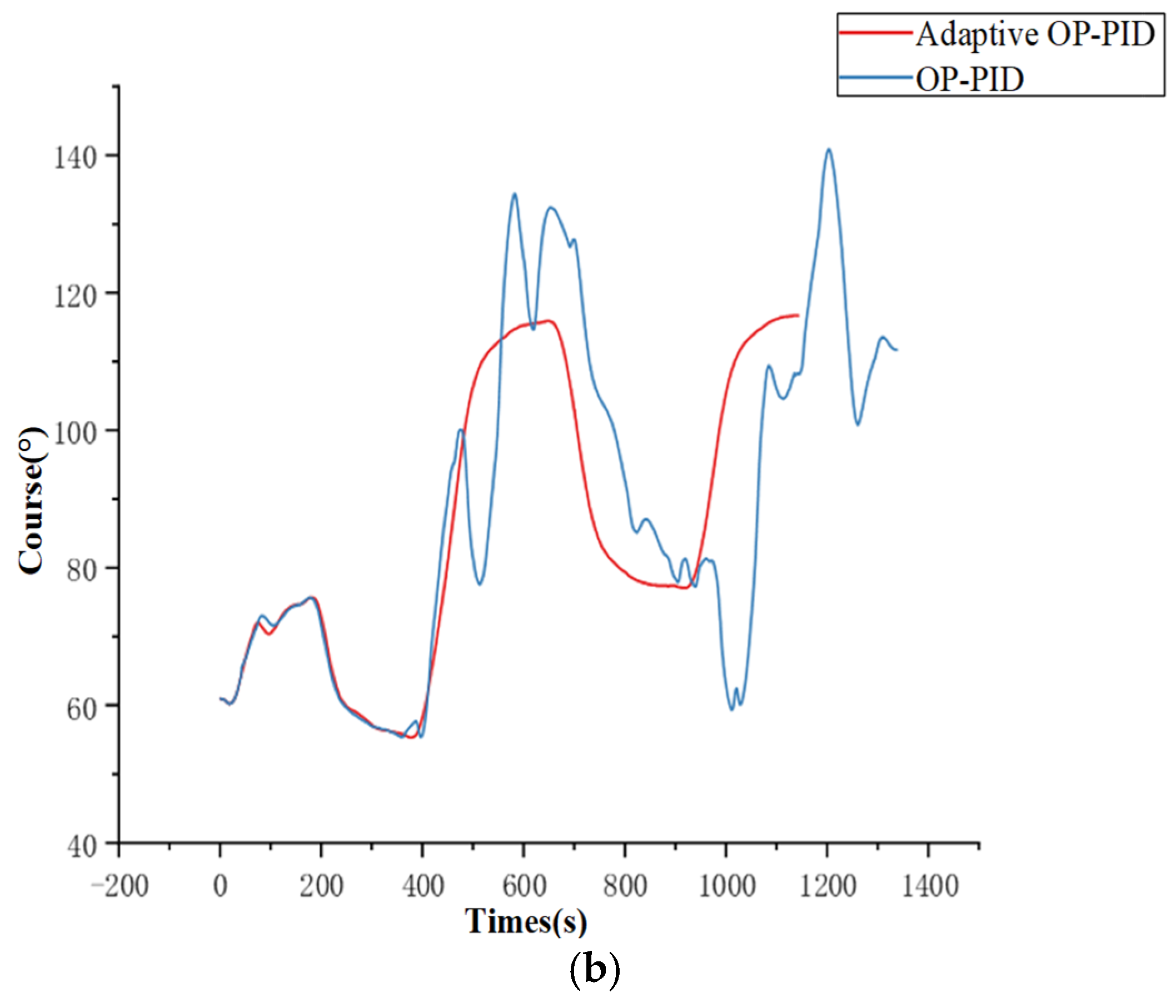
5.2. Track Control Simulation

Set the wind speed to 4 m/s, current speed to 0.5 m/s, wave height to 0.2 m, and directions all to 000 for the simulation environment. Set the planned route on the electronic chart of the maneuvering simulator, as shown in

Table 6. The value of m corresponds to the wind speed table.

Way Point	Latitude	Longitude	Course	Distance/nm
0	30° 08.360 N	122° 30.540 E	/	/
1	30° 08.583 N	122° 31.500 E	075	0.859
2	30° 09.026 N	122° 32.260 E	056	0.793
3	30° 08.652 N	122° 33.186 E	115	0.884
4	30° 08.846 N	122° 34.216 E	077	0.911
5	30° 08.532 N	122° 34.938 E	116	0.699

, and add Ship Type I, with the initial ship position set to (30° 08.359 N, 122° 30.710 E) and an initial course of 060, an initial speed of 12 knots, and a slow deceleration. Take the OP-PID and Adaptive OP-PID control to navigate the ship along the planned route and when the ship reaches the last waypoint, the test ends. Repeat the test once again with Ship Type II under the same conditions.

The track control process can be displayed in the chart of the maneuvering simulator, as shown in Figure 16 and Figure 17, which are the track charts of Ship Type I and Ship Type II under the control of the two algorithms, respectively. The black broken line is the planned route and the white rectangle is the historical trajectory of the ship.

According to Figure 16 and Figure 17, it can be seen that the OP-PID could still track the planned routes well at the beginning of the experiment under interference and speed variation but, as the speed decreased, the PID parameters could not adapt to the new motion state and the track deviation increased significantly at the third-way point. For both Ship Types I and II, the Adaptive OP-PID with changing control parameters according to speed has better control effects, can track the planned routes stably, and has higher control precision in small curvature than large. The maximum track deviation of the Adaptive OP-PID in Figure 18a is 116 m, which, for the OP-PID, is 131 m. In Figure 18b, the maximum track deviation of the Adaptive OP-PID is 100 m, which, for the OP-PID, is 186 m. Clearly, the track deviation of the Adaptive OP-PID is smaller than that of the OP-PID. Especially for Ship Type II, the control effect of the Adaptive OP-PID is more precise. As shown in Figure 19, the ship controlled by the Adaptive OP-PID has a smooth change in course at each way point, with no overshoot or oscillation, while the ship controlled by the OP-PID has a certain degree of overshoot and oscillation.

6. Conclusions

In this paper, the forgetting factor was introduced to improve the recursive least squares method, which not only avoids the disadvantage of the ordinary least squares method that cannot be identified online but also compensates for the defect of the recursive least squares method that the update speed decreases with the accumulation of data. The recursive least squares algorithm with forgetting factor was then used to identify the parameters of the ship maneuvering motion model and the ship maneuvering indexes K and T were identified online. The data required for parameter identification were obtained from the maneuvering simulator. The identification process and the results of different forgetting factors were compared to analyze their influence on parameter identification and the identification results were used to calculate the OP-PID parameters in real-time. An adaptive OP-PID course control method was proposed. Finally, the maneuvering simulator, which is more suitable for the actual ship motion, was used as the simulation platform and the course and heading control simulation tests were carried out under different types and environments with the Adaptive OP-PID and the OP-PID in the existing research. The results show that the Adaptive OP-PID can be applied to ship motion control in different ship types and environments. Under the same conditions, the performance of the proposed algorithm is better than that of the optimal PID in terms of heading stability, heading convergence time, and heading deviation. In other words, the parameter identification method of the ship maneuvering motion model with forgetting factor has higher accuracy in theory and the Adaptive OP-PID course control method designed based on it is better than the OP-PID course control method based on statistical formula calculation in theory. It should be noted that both recursive least squares and OP-PID are quite mature theories at present. This paper only attempts to apply the least squares with forgetting factor to the parameter identification of the responsive ship maneuvering motion model and use the identified parameters to design the adaptive optimal control method. Due to the recursive process employed by RLS, it does not require frequent matrix multiplication operations. Therefore, compared to the Kalman filter, RLS has a lighter computational burden, especially noticeable in high-dimensional state estimation. Additionally, RLS does not require an accurate state-space model as the Kalman filter does. In contrast to ordinary least squares, the inclusion of a forgetting factor allows RLS to dynamically adjust the weight of historical data, improving its adaptability. However, RLS also has drawbacks, such as its sensitivity to noise, which can lead to unstable parameter estimates when data quality is poor.

Certainly, this paper only combines the K and T values obtained from statistical formulas and those identified through FFRLS with OP-PID and conducts longitudinal heading and trajectory control experiments using the ship maneuvering simulator. However, no lateral comparisons with other control methods, such as sliding mode control, have been made and the ship maneuvering simulator does not allow for comparative experiments under different external disturbances. Future work will focus on addressing these shortcomings and making improvements.

References

1. Seung, J.L.; Kwang, H.J.; Namkug, K.; Jaeyong, L. A comparison of regression models for the ice loads measured during the ice tank test. Brodogradnja. 2023, 74, 1–15. [Google Scholar] [CrossRef]
2. Mustafayev, V.O.; Mammadov, E.D. Diving vessel speed determination during towing tests. Int. J. Tech. Phys. Probl. Eng. 2024, 16, 333–336. [Google Scholar] [CrossRef]
3. Atasayan, E.; Milanov, E.; Dursun, A.A. Application of an offline grey box method for predicting the maneuvering performance. Brodogradnja. 2024, 75, 75304. [Google Scholar] [CrossRef]
4. Allotta, B.; Costanzi, R.; Pugi, L.; Ridolfi, A. Identification of the main hydrodynamic parameters of Typhoon AUV from a reduced experimental dataset. Ocean. Eng. 2018, 147, 77–88. [Google Scholar] [CrossRef]
5. Yin, Q.; Cai, J.; Gong, X.; Ding, Q. Local parameter identification with neural ordinary differential equations. Appl. Math. Mech. 2022, 43, 1887–1900. [Google Scholar] [CrossRef]
6. Luigi, B.; Felice, I.; Ewa, B.W. Weighted least squares collocation methods. Appl. Numer. Math. 2024, 203, 113–128. [Google Scholar] [CrossRef]
7. Sabet, M.T.; Fathi, A.R.; Mohammadi, H.R. Optimal design of the Own Ship maneuver in the bearing-only target motion analysis problem using a heuristically supervised Extended Kal-man Filter. Ocean Eng. 2016, 123, 146–153. [Google Scholar] [CrossRef]
8. Triantafyllou, M.; Bodson, M.; Athans, M. Real time estimation of ship motions using Kalman filtering techniques. IEEE J. Ocean Eng. 2003, 8, 9–20. [Google Scholar] [CrossRef]
9. Cosmo, L.; Minello, G.; Bicciato, A.; Bronstein, M.; Rodola, E.; Rossi, L.; Torsello, A. Graph Kernel Neural Networks. IEEE Trans. Neural Netw. Learn. Syst. 2024, 1–14. [Google Scholar] [CrossRef] [PubMed]
10. Esra, Y.; Taskin, K. Deep convolutional neural networks for ship detection using refined DOTA and TGRS-HRRSD high-resolution image datasets. Adv. Space Res. 2024, in press. [Google Scholar] [CrossRef]
11. Gao, H.; Zou, Z.; Xia, L. Application of the NIPC-based uncertainty quantification in prediction of ship maneuverability. J. Mar. Sci. Technol. 2021, 26, 555–572. [Google Scholar] [CrossRef]
12. Dong, Q.; Wang, N.; Song, J.; Hao, L.; Liu, S.; Han, B.; Qu, K. Math-data integrated prediction model for ship maneuvering motion. Ocean Eng. 2023, 285, 115255. [Google Scholar] [CrossRef]
13. Ning, W.; Hui, W.; Yu, Z.; Jia, S.; Ye, L.; Li, H. Self-organizing data-driven prediction model of ship maneuvering fast-dynamics. Ocean Eng. 2023, 288, 115989. [Google Scholar] [CrossRef]
14. Wang, N.; Kong, X.; Ren, B.; Hao, L.; Han, B. SeaBil: Self-attention-weighted ultrashort-term deep learning prediction of ship maneuvering motion. Ocean Eng. 2023, 287, 115890. [Google Scholar] [CrossRef]
15. Fossen, T.I. Handbook of Marine Craft Hydrodynamics and Motion Control; John Willy & Sons: Hoboken, NJ, USA, 2011. [Google Scholar]
16. Buerger, J.; Cannon, M. A Constraint Homotopy Active Set Solver for Linear–Quadratic Optimal Control. IEEE Trans. Autom. Control 2024, 69, 7205–7210. [Google Scholar] [CrossRef]
17. Liu, J.; Huang, L.; Yu, D.; Xu, L.; He, Y. The control method for ship tracking when navigating through narrow and curved sections. Appl. Ocean Res. 2024, 145, 103943. [Google Scholar] [CrossRef]
18. McCue, L. Handbook of Marine Craft Hydrodynamics and Motion Control. IEEE Control Syst. Mag. 2016, 36, 78–79. [Google Scholar] [CrossRef]
19. Cao, B. Study on Ship Motion Control Simulation System Based on Model Parameter Identification. Ph.d. Thesis, Ji Lin University, Changchun, China, 2012. [Google Scholar]
20. He, Y.; Zhao, X.; Huang, L.; Xu, L.; Liu, J. Control method for the ship track and speed in curved channels. Brodogradnja 2024, 75, 1–27. [Google Scholar] [CrossRef]
21. Zhang, W.; Zhang, C.; Zheng, C. Design of improved line-of-sight guidance law based on aircraft visual information. Syst. Eng. Electron. 2024, 46, 2779–2788. [Google Scholar]
22. Yu, C.; Zhu, J.; Hu, Y.; Zhu, H.; Wang, N.; Guo, H.; Zhang, Q.; Liu, S. Prescribed-time observer-based sideslip compensation in USV line-of-sight guidance. Ocean Eng. 2024, 298, 117177. [Google Scholar] [CrossRef]
Figure 1. Geodetic coordinate system and ship coordinate system.
Jmse 13 00753 g001
Figure 2. Ship plane coordinate system.
Jmse 13 00753 g002
Figure 3. Iterative flow chart of parameter identification.
Jmse 13 00753 g003
Figure 4. The forgetting factor is 0.98 in the parameter identification process. (a) Parameter values; (b) Value of error.
Jmse 13 00753 g004
Figure 5. The forgetting factor is 0.99 in the parameter identification process. (a) Parameter values; (b) Value of error.
Jmse 13 00753 g005
Figure 6. 20°/20° Z-type test. (a) Z-type test of recursive least squares with forgetting factor; (b) Z-type test of ordinary least squares.
Jmse 13 00753 g006
Figure 7. Adaptive OP-PID control principle.
Jmse 13 00753 g007
Figure 8. K and T values vary with speed v.
Jmse 13 00753 g008
Figure 9. Indirect track control.
Jmse 13 00753 g009
Figure 10. Course control of Ship Type I. (a) OP-PID control; (b) Adaptive OP-PID control.
Jmse 13 00753 g010
Figure 11. Course control of Ship Type II. (a) OP-PID control; (b) Adaptive OP-PID control.
Jmse 13 00753 g011
Figure 12. Course change curve. (a) Ship Type I; (b) Ship Type II.
Jmse 13 00753 g012aJmse 13 00753 g012b
Figure 13. Course control of Ship Type I. (a) OP-PID control; (b) Adaptive OP-PID control.
Jmse 13 00753 g013
Figure 14. Course control of Ship Type II. (a) OP-PID control; (b) Adaptive OP-PID control.
Jmse 13 00753 g014
Figure 15. Course change curve. (a) Ship Type I; (b) Ship Type II.
Jmse 13 00753 g015
Figure 16. Track control simulation of Ship Type I. (a) Adaptive OP-PID; (b) OP-PID.
Jmse 13 00753 g016aJmse 13 00753 g016b
Figure 17. Track control simulation of Ship Type II. (a) Adaptive OP-PID; (b) OP-PID.
Jmse 13 00753 g017
Figure 18. Track deviation. (a) Ship Type I; (b) Ship Type II.
Jmse 13 00753 g018
Figure 19. Change of course. (a) Ship Type I; (b) Ship Type II.
Jmse 13 00753 g019aJmse 13 00753 g019b