A Numerical Simulation-Based Study on the Impact of Changes in Flow Rate of a Typical River Emptying into the Northern Yellow Sea on Water Environment of the River Estuary and Coastal Waters

Abstract

In this study, a numerical simulation method was used to explore the impact of changes in riverine runoff input flow variations on the marine environmental dynamics in the northern Yellow Sea of China. Based on the depth-averaged two-dimensional shallow water equations, a hydrodynamic and water quality coupling model was established to simulate the changes of the water environmental indicators under five conditions. Validation against filed-measured data confirmed the model’s great accuracy and stability. The findings show that interception activities had a relatively small impact on hydrodynamic conditions, and the changes in velocity did not exceed 10 cm/s; however, the salinity changed significantly. As the interception rate increased, the moving distance of the isohaline with a value of 5 towards the estuary gradually increased, with a maximum distance of 3420 m. Meanwhile, the amount of reduction of the area of the envelope curve with a salinity of 26.8 gradually increased, with a peak areal reduction rate of 10.7%. The amount of changes in nutrient concentration was related to the interception rate and the distance of a station from the estuary. The maximum percentages of changes in inorganic nitrogen and inorganic phosphorus contents were 5.39% and 6.34%, respectively. This study provides a technical methodology for evaluating the impacts of analogous riverine runoff variations on estuarine and adjacent ecosystems.

1. Introduction

In general, coastal estuaries are areas with a high degree of biodiversity, where freshwater runoff replenishment plays a vital role in the protection of biomass, the impact on the ecological environment and its restoration. The river investigated in this paper is one of the main rivers emptying into the northern Yellow Sea of China [1]. The river estuary has abundant biological resources and serves as a major habitat, migration path, and supply station for rare birds in China, which is quite influential around the globe. In recent years, due to global warming, the originally stable water circulation has been seriously damaged [2]. In addition, industrial and agricultural development in the upper reaches of the river increased the demand for water, so various water conservancy projects were constructed along the river, such as reservoirs, dams, and water interception works, leading to significant changes in the amount of freshwater entering the sea through the estuary [3]. This will have a certain impact on the biodiversity and ecological stability of the entire estuarine area, including the hydrodynamic environment, salinity field distribution, nutrient input, plankton community and biomass, fish distribution, etc., which means that such reduction in the amount of freshwater entering the sea is one of the main reasons for the changes in the ecosystem of the estuarine area and surrounding seawater [4]. The most direct impact is that on hydrodynamics and the water quality environment of the estuarine area and nearshore waters. Therefore, it is crucial to accurately predict and scientifically analyze the water environment conditions in the estuary area affected by changes in runoff. This study is of important theoretical and practical significance for protecting water environment quality, avoiding aquatic ecological disasters, and ensuring the abundance of biological resources in the estuary area.

In recent years, many researchers have carried out studies on related issues using a variety of methods, including pure monitoring methods, artificial intelligence-based methods, physical model methods, and numerical simulation methods. Numerical simulation methods have various advantages, such as high prediction accuracy, timeliness, time saving, labor saving, and cost saving, so they have been favored by a great number of researchers. Rostamzadeh-Renani M., Rostamzadeh-Renani R., and Baghoolizadeh MKAN investigated the impact of vortex generators on the hydrodynamic performance of submarines at high angles of attack using multi-objective optimization and computational fluid dynamics [5]. In the findings, computational fluid dynamics (CFD) analysis was combined with a multi-objective genetic algorithm (MOGA), providing an accurate understanding on the impact of the ideal design of VG on the hydrodynamic performance of submarines, and putting forward a great technical method for the manufacturing, performance research, and development of high-performance technical equipment for national defense. Gong W., Lin Z., and Zhang H. et al. [6], based on the cross-wavelet and wavelet coherence analysis, investigated the responses of salt intrusion to different forces, including tidal range, river discharge, and alongshore and cross-shore winds, in different timescales in their study. The findings showed that tides served as the most important factor affecting the interannual variation of salt intrusion. Shou W., Zong H., and Ding P. conducted a numerical simulation-based study on the impact of the Yellow River runoff emptying into the sea on water circulation in the Yellow River estuary and its adjacent waters during summer [7]. Rostamzadeh-Renani M., Baghoolizadeh M., and Sajadi S. M. et al. optimized the flap geometry and position based on a multi-objective CFD method [8], while reducing drag and lift. Through parameter selection, design variable generation, and objective function creation, they successfully achieved the goal of minimizing energy consumption. The study can be considered an innovation in the field of aerodynamic simulation. Gao Z., Yang J., and Cui W. et al. analyzed the impact of a sharp decline or even a cutoff of the Yellow River runoff emptying into the sea on the marine ecological environment in the estuary in detail on the basis of the measured data from many years [9], indicating that the sharp decrease in the runoff emptying into the sea has changed the marine habitat elements, which affected marine organisms, leading to a decline in marine fishery productivity and the extinction of some species. Some researchers also used artificial intelligence-based methods, such as Rostamzadeh-renani M., Baghoolizadeh M., and Rostamzadeh-renani R. et al., who predicted and analyzed the impact of special geometric designs on automobile wake control using artificial neural networks and genetic algorithms [10]. In addition, Zhao G., Zhang Z., and Liang R. et al. studied the impact of runoff changes at the Beimen River estuary in the northwest of Hainan Island on the water environment of the estuarine reach [11]. Nguyen H. Q., Jun S., and Hiroto H. et al. investigated the temporal and spatial changes in turbidity of waters and the major factors affecting its change pattern using remote sensing data [12]. On the basis of the correlation between field measurement data and the red band of the Operational Land Imager (OLI) on Landsat 8, a retrieval algorithm for turbidity was developed, and the Simulating Waves Nearshore (SWAN) model was used to compute the main factor affecting turbidity in shallow waters—bottom shear stress. In addition, the relationship between turbidity and rainfall, as well as that between wind-induced bottom shear stress and turbidity, were analyzed, laying a foundation for more detailed studies on the impact of turbidity changes, a major water quality indicator for Jinlan Bay and tidal lagoon waters, on the water environment, and for the prediction of such changes. Zhu Y., Huang X., and Xie R. et al. conducted an experimental study on the impact of the runoff of the Minjiang River on saltwater intrusion in the estuary and applied the study findings [13]. Liang J., Xu Y., and Zhang W. et al. studied the impact of changes in the runoff rates of the Xijiang River and the Beijiang River in the Pearl River Delta region on salt tides in the tidal estuaries, basing their study on the salinity convection–diffusion equation [14]. Gong Y. and Zhang M. simulated the hydrodynamic characteristics of the Liaohe River estuary using a three-dimensional hydrodynamic model [15] (FVCOM). Wu Q., Zhang W., and Wang X., proceeding from the changes in the expansion direction and range of the Yangtze River runoff emptying into the sea on seasonal and inter-annual scales [16], systematically studied the impact of nutrients carried by the Yangtze River runoff on chlorophyll in the estuary and the possible physical mechanism of the impact of ENSO years on chlorophyll in the Yangtze River estuary based on a statistical analysis method and a two-layer nested high-resolution physical–biogeochemical coupling model. Wang Y., Liu Z., and Zhang Y. et al. carried out a comprehensive survey with six voyages in Jiaozhou Bay and investigated the spatiotemporal variation characteristics of surface seawater temperature, salinity, nutrient content and chlorophyll a concentration [17]. The above research findings undoubtedly provided us with valuable experience and techniques, data, and inspirations for our later studies.

Freshwater runoff replenishment plays an important role in protecting the ecological environment and carrying out systematic restoration. Moreover, there are few numerical simulation-based prediction studies and published findings for this typical river entering the northern Yellow Sea. In order to fully understand and describe the impact of river interception on the relevant water environment indicators of the sea area, numerical simulation and a multi-condition scheme design were used in this paper to quantitatively calculate the hydrodynamic indicators, salinity, and distribution of the nutrient content field in the estuary and nearshore waters before and after river interception for irrigation in the corresponding water periods, and analyze the extent of any impact on the basis of the natural conditions of the water area, runoff rates in multiple years, water environment data and supplementary survey data on the current situation.

Based on the specific research strategy of this paper, a depth-averaged two-dimensional shallow water model (two-dimensional shallow water equations) for the estuary and nearshore sea area was established, which was then verified with hydrological observation values from 2024. It was found through verification that the simulated values were in good agreement with the measured values, indicating that the model has great accuracy, stability, and universality; the calculation results before and after river interception for irrigation were compared and analyzed. Meanwhile, the movement and changes of the 5-isohaline after water interception were investigated in an in-depth manner, which convincingly explained the quantitative impact of water interception for irrigation on the water environment of the estuary and nearshore sea area. This study presents a technical method and important quantitative data that can accurately predict the possible impact of river water interception for irrigation on estuarine organisms and help management authorities understand changes in the water environment and ecological environment within the scope of the estuary in real time, thereby helping them make decisions regarding ecological restoration of the estuary ecosystem and providing related compensation for losses suffered by fisheries.

2. Material and Method

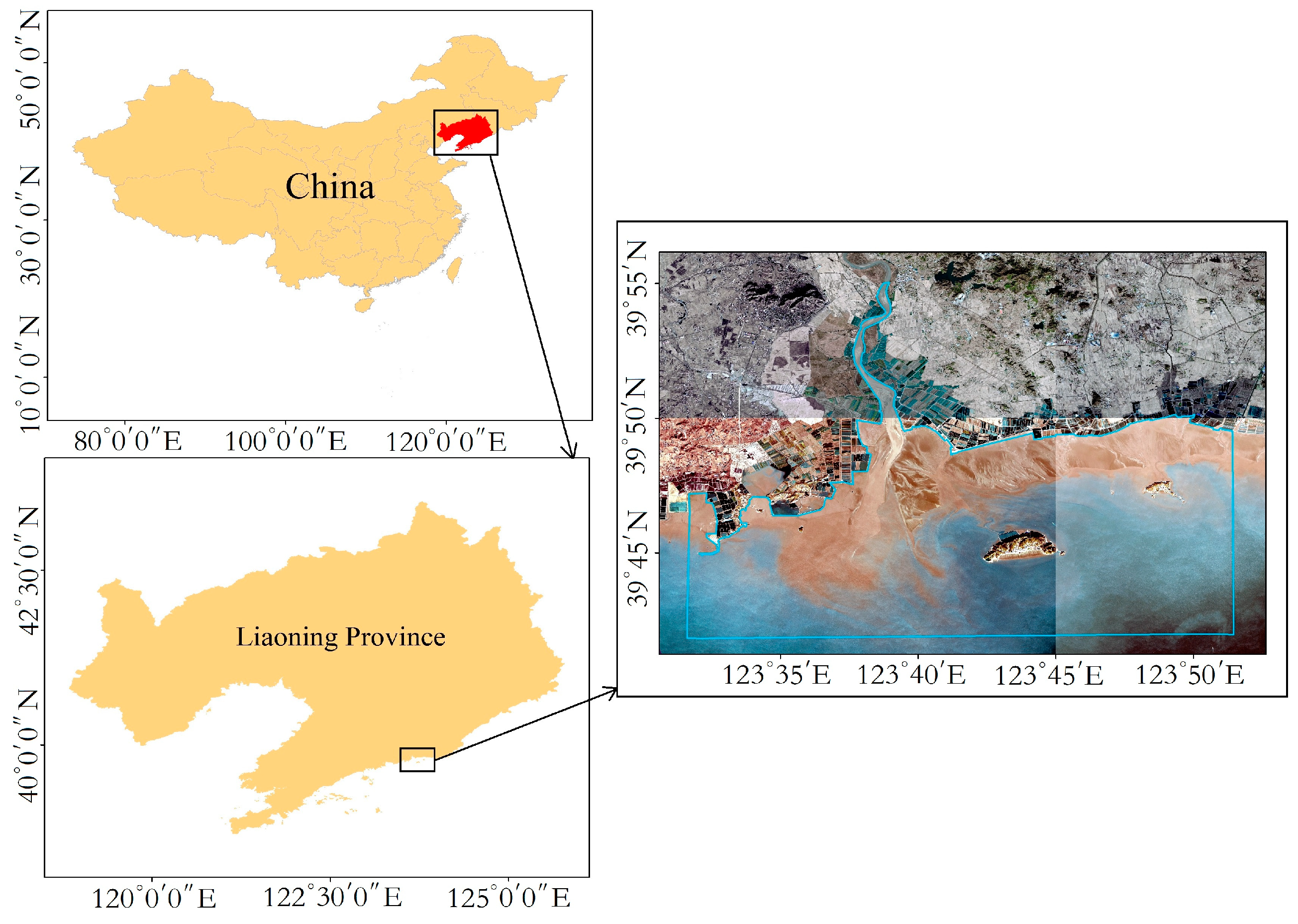
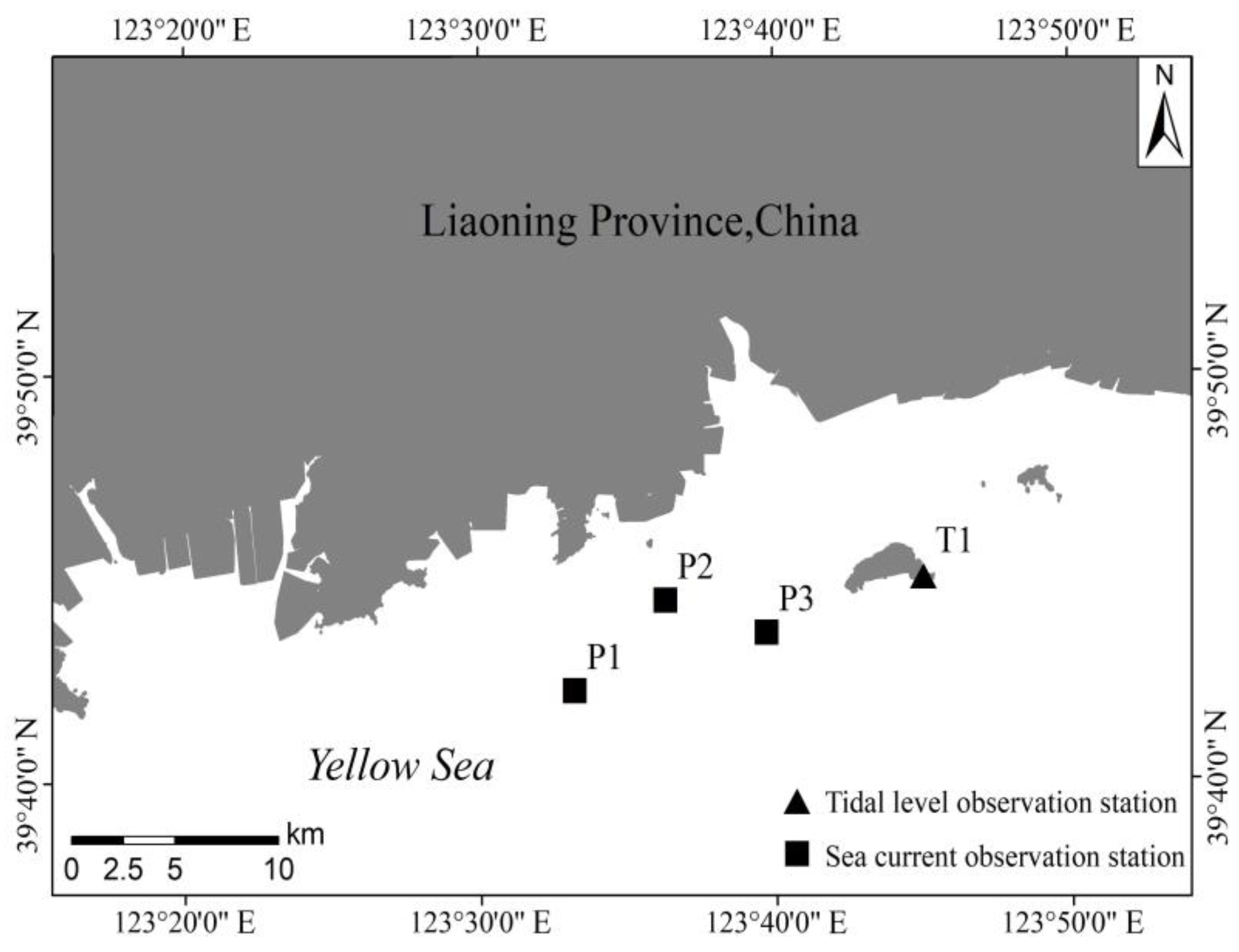
2.1. Investigated Water Area and Observational Data

The location and scope of the specific investigated water area in this paper are shown in Figure 1 below. The project team set up a temporary tide observation station and three synchronous continuous current observation stations in the coastal waters of the northern Yellow Sea. The specific coordinates of the stations are shown in

Table 1. Coordinates of observation stations.

Station	Longitude	Latitude
T1	123°45′0″ E	39°45′0″ N
P1	123°33′10.558″ E	39°42′14.462″ N
P2	123°36′15.952″ E	39°44′26.600″ N
P3	123°39′41.122″ E	39°43′38.126″ N

and their locations are shown in Figure 2.

2.2. Model and Method

2.2.1. Hydrodynamic Model

The investigated area is located in the coastal waters of the northern Yellow Sea in Liaoning Province, China (see Figure 1). A vertically averaged two-dimensional shallow water model was used to reproduce and predict the hydrodynamic environment conditions under various design schemes in the river estuary in order to numerically reproduce and predict the movement of water flow in the nearby waters [18,19,20,21], thereby providing a background field for the subsequent prediction and simulation of the impact of runoff changes caused by river interception on the distribution of salinity and nutrient content in the estuary. Based on the Reynolds-averaged three-dimensional Navier–Stokes equations for incompressible fluids, the horizontal momentum equation and continuity equation were integrated within the total water depth [0,h], after which the following two-dimensional depth-averaged shallow water equations could be obtained:

$${\displaystyle \frac{\partial h}{\partial t}}+{\displaystyle \frac{\partial h\overline{u}}{\partial x}}+{\displaystyle \frac{\partial h\overline{v}}{\partial y}}=hS$$

(1)

$$\begin{array}{l}{\displaystyle \frac{\partial h\overline{u}}{\partial t}}+{\displaystyle \frac{\partial h{\overline{u}}^2}{\partial x}}+{\displaystyle \frac{\partial h\overline{v}\overline{u}}{\partial y}}=f\overline{v}h-gh{\displaystyle \frac{\partial \eta }{\partial x}}-{\displaystyle \frac{h}{{\rho }_0}}{\displaystyle \frac{\partial p_a}{\partial x}}-{\displaystyle \frac{g{h}^2}{2{\rho }_0}}{\displaystyle \frac{\partial \rho }{\partial x}}+{\displaystyle \frac{{\tau }_{sx}}{{\rho }_0}}-{\displaystyle \frac{{\tau }_{bx}}{{\rho }_0}}\\ -{\displaystyle \frac{1}{{\rho }_0}}\left[{\displaystyle \frac{\partial s_{xx}}{\partial x}}+{\displaystyle \frac{\partial s_{xy}}{\partial y}}\right]+{\displaystyle \frac{\partial }{\partial x}}\left(h{T}_{xx}\right)+{\displaystyle \frac{\partial }{\partial y}}\left(h{T}_{xy}\right)+h{u}_{s}S\end{array}$$

(2)

$$\begin{array}{l}{\displaystyle \frac{\partial h\overline{v}}{\partial t}}+{\displaystyle \frac{\partial h{\overline{v}}^2}{\partial x}}+{\displaystyle \frac{\partial h\overline{u}\overline{v}}{\partial y}}=f\overline{u}h-gh{\displaystyle \frac{\partial \eta }{\partial y}}-{\displaystyle \frac{h}{{\rho }_0}}{\displaystyle \frac{\partial p_a}{\partial y}}-{\displaystyle \frac{g{h}^2}{2{\rho }_0}}{\displaystyle \frac{\partial \rho }{\partial y}}+{\displaystyle \frac{{\tau }_{sy}}{{\rho }_0}}-{\displaystyle \frac{{\tau }_{by}}{{\rho }_0}}\\ -{\displaystyle \frac{1}{{\rho }_0}}\left[{\displaystyle \frac{\partial s_{yx}}{\partial x}}+{\displaystyle \frac{\partial s_{yy}}{\partial y}}\right]+{\displaystyle \frac{\partial }{\partial x}}\left(h{T}_{yx}\right)+{\displaystyle \frac{\partial }{\partial y}}\left(h{T}_{yy}\right)+h{v}_{s}S\end{array}$$

(3)

where t, x, and y are temporal and spatial coordinates; η is free water surface level (m); h = η + d is total water depth (m), d is static water depth (m); ū and $\overline{v}$ are vertical average velocitys in the directions of x and y; ρ is water body density (kg/m³); ρ₀ is relative density of the water body; S is source-sink flow value; p_a is atmospheric pressure (Pa); u_s and v_s are source-sink velocity values;$f=2\omega \sin \phi$, where $\omega$ is rotational angular velocity of the earth and φ is geographic latitude; (τ_sx, τ_bx) and (τ_sy, τ_by) are the components of the surface wind and seafloor shear stress in the directions of x and y; T_xx, T_xy, T_yx, and T_yy are lateral stresses, including viscous stress, turbulent friction, and convection friction.

Interactions between waves and currents lead to complex turbulence phenomena, which have an important impact on the location and transport of nutrients, distribution of temperature and salinity indicators, and transport of sediment [22]. The turbulence caused by wave–current interactions is mainly handled through the comprehensive consideration of horizontal eddy viscosity parameterization, wave radiation stress coupling, and bottom friction correction. In this paper, the turbulent eddy viscosity coefficient was introduced. The horizontal eddy viscosity coefficient was dynamically given based on the Smagorinsky model. The formula is related to the grid scale and water flow gradient. The specific configuration is shown in the model settings.

Equations (1)–(3) constitute the basic control equations for solving the hydrodynamic background field of the estuarine area. In order to ensure the uniqueness of the solution, definite conditions must be given, including initial and boundary conditions. The following scheme is given as:

(1)

Initial conditions

The cold start mode was adopted, meaning that the initial conditions were considered to be irrelevant to the final calculation results. In this study, the values of initial velocity and tide level are both 0.

(2)

Boundary conditions

In this paper, two boundary conditions are given, including closed boundary and open boundary conditions.

The closed boundary is the boundary where the land and water meet, which is determined by the coastline and islands. The normal velocity is zero at the closed boundary.

Based on the investigated area, the northern boundary of the tidal river was set as the flow open boundary condition, which was given based on the multi-year average flow. The southern boundary, as well as the east- and westsides, were set as open boundaries, and the following formula of harmonic tidal constituents was used to calculate the open boundary conditions of the tidal level time series. In addition, for tidal flats, the location where the land and water meet varies with the rise and fall of the tide level. In this model, dryness/wetness variation of the grid nodes within the moving boundaries were taken into consideration [23,24,25].

The formula of harmonic tidal constituents used to calculate the open boundary conditions of the tidal level time series is provided below:

$$\eta (x,y,t)={\displaystyle \sum _{k=1}^m{f}_k}{H}_k\cos \left[w_{k}t+{\left(v_0+u\right)}_k-g_k\right]$$

(4)

where k is the tidal constituent sequence number; m is the numberof tidal constituents; ${\omega }_k$ is the angular velocity of each tidal constituent; H_k and g_k are the amplitude and retardation angle of each tidal constituent, i.e., the harmonic constant; f_k and u_k are the intersection factor and retardation angle correction of each tidal constituent, respectively; ${(V_0+u)}_k$ is the astronomical initial phase of each tidal component.

(3)

Numerical discretization of model control equationss

A CC-based finite volume method was used to discretize the partial differential equations for model control. In order to increase the accuracy of model verification and parameter calibration, the density of the meshes in the key areas near the measuring stations was increased to improve the adaptability of the program system to shoreline changes and the terrain, as well as to improve the calculation accuracy.

2.2.2. Water Environment Model

On the basis of an accurate hydrodynamic background field, a convection–diffusion transport model for water environment was established for the estuary and coastal waters, where some indexes (salinity and nutrient concentrations) of the waterbody were the major unknown data. The equation is shown below:

$${\displaystyle \frac{\partial C}{\partial t}}+u{\displaystyle \frac{\partial C}{\partial x}}+v{\displaystyle \frac{\partial C}{\partial y}}=E_x{\displaystyle \frac{\partial {}^{2}C}{\partial x^2}}+E_y{\displaystyle \frac{\partial {}^{2}C}{\partial y^2}}+S$$

(5)

where E_x and E_y are the water diffusion coefficients in the horizontal directions; C is concentration, a water quality indicator; S is the source-sink term.

2.3. Grid Creation and Model Settings

2.3.1. Grid Creation

The computational grid was generated by the SMS (Surface Water Model System 10.1). This grid generator features flexible and variable resolution in the horizontal direction of the grid, showcases a great gradient, and can generate high-quality smooth grids in locations where circum-island currents are likely to be formed. In addition, it can increase mesh density in areas with complex terrains, such as coastal areas, estuaries, and wetlands in offshore areas. A total of 3546 unstructured triangular grid nodes and 6557 grid cells were generated, and the minimum mesh scale in the river channel was about 35 m. Mesh distribution is shown in Figure 3.

2.3.2. Model Settings

In the model, the computing time step was adjusted according to the CFL conditions to ensure that the maximum time step was 30 s when the model computation converged. The bottom friction was controlled by Manning’s number, and the specific value was 33–45 m^1/3/s. The simulation period was from 5 June to 22 June 2024. The terrain data were obtained by combining the measured data of the river channel terrain and the terrain with the maximum resolution extracted from a global database. The diffusion coefficient is related to the turbulence intensity and is proportional to the turbulent eddy viscosity coefficient. In many applications, a constant eddy viscosity can be used for horizontal stress terms. Alternatively, Smagorinsky (1963) [26] proposed to express sub-grid scale transports by an effective eddy viscosity related to a characteristic length scale. The sub-grid scale eddy viscosity is given by [26,27,28], and is specifically expressed as follows:

$$A=c_s^2{l}^2\sqrt{2S_{ij}{S}_{ij}}$$

(6)

where c_s is a constant, l is a characteristic length, and the deformation rate is given by

$$S_{ij}={\displaystyle \frac{1}{2}}\left({\displaystyle \frac{\partial u_i}{\partial x_j}}+{\displaystyle \frac{\partial u_j}{\partial x_i}}\right)$$

(7)

3. Results

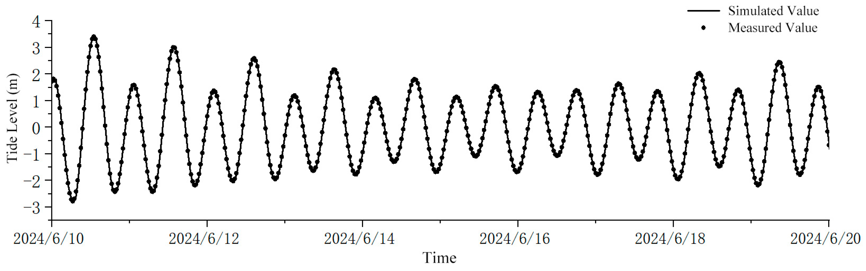
3.1. Model Verification Results

The verification data included the flowrate and direction data from the three observation stations, which were collected synchronously and continuously from 20 June to 21 June 2024, as well as the tide level observation data from the tide level observation station, which have been collected for 10 consecutive days. In order to improve the reliability of the model, the hydrodynamic module was verified by using the measured values, while continuous salinity observations were conducted at the stations for the salinity module. The results of verification and comparison of the simulation data and the measurement data are shown in Figure 4, Figure 5 and Figure 6 below. A comparison of the simulated values and the measured values indicates that they are in good agreement with each other; the curve is smooth and has no abrupt change, and the tidal characteristics are well described. The results suggest that the parameter settings are reasonable and the model is stable, which can meet the simulation requirements of various hydrodynamic and water environment design schemes in the later stage.

3.2. Simulation Results Under Various Conditions

The simulation conditions were set based on the five interception schemes. Due to the limited space of the paper, the following water flow, salinity, and nutrient distribution results (Figure 7, Figure 8, Figure 9 and Figure 10) only show the planar distribution of the water environment simulation results at different time points under three typical conditions. For the sake of clarity,

Table 2. Flow rates and interception rates under the simulation schemes.

Simulation Scheme	Condition 1	Condition 2	Condition 3	Condition 4	Condition 5
Flow rate (m3/s)	97.500	82.290	68.650	60.090	46.455
Interception rate	0	16%	30%	38%	52%

shows the correspondence between flow rates and interception rates under the five simulation conditions.

3.3. Analysis of Water Environment Changes Under Different Schemes

The changes in salinity of the planar positions under various simulation conditions are not very obvious in the above planar diagram. In order to show the amount of changes more clearly and obviously, three characteristic representative locations in the tidal area of the estuary were selected, and the results of comparison of the water environment-simulated values under five different conditions were given for the selected positions. The coordinates of the characteristic representative locations are shown in

Table 3. Coordinates of characteristic representative stations.

Station	Longitude	Latitude
1#	123°33′10.558″ E	39°42′14.462″ N
2#	123°39′13.313″ E	39°49′29.110″ N
3#	123°38′52.020″ E	39°55′1.020″ N

below.

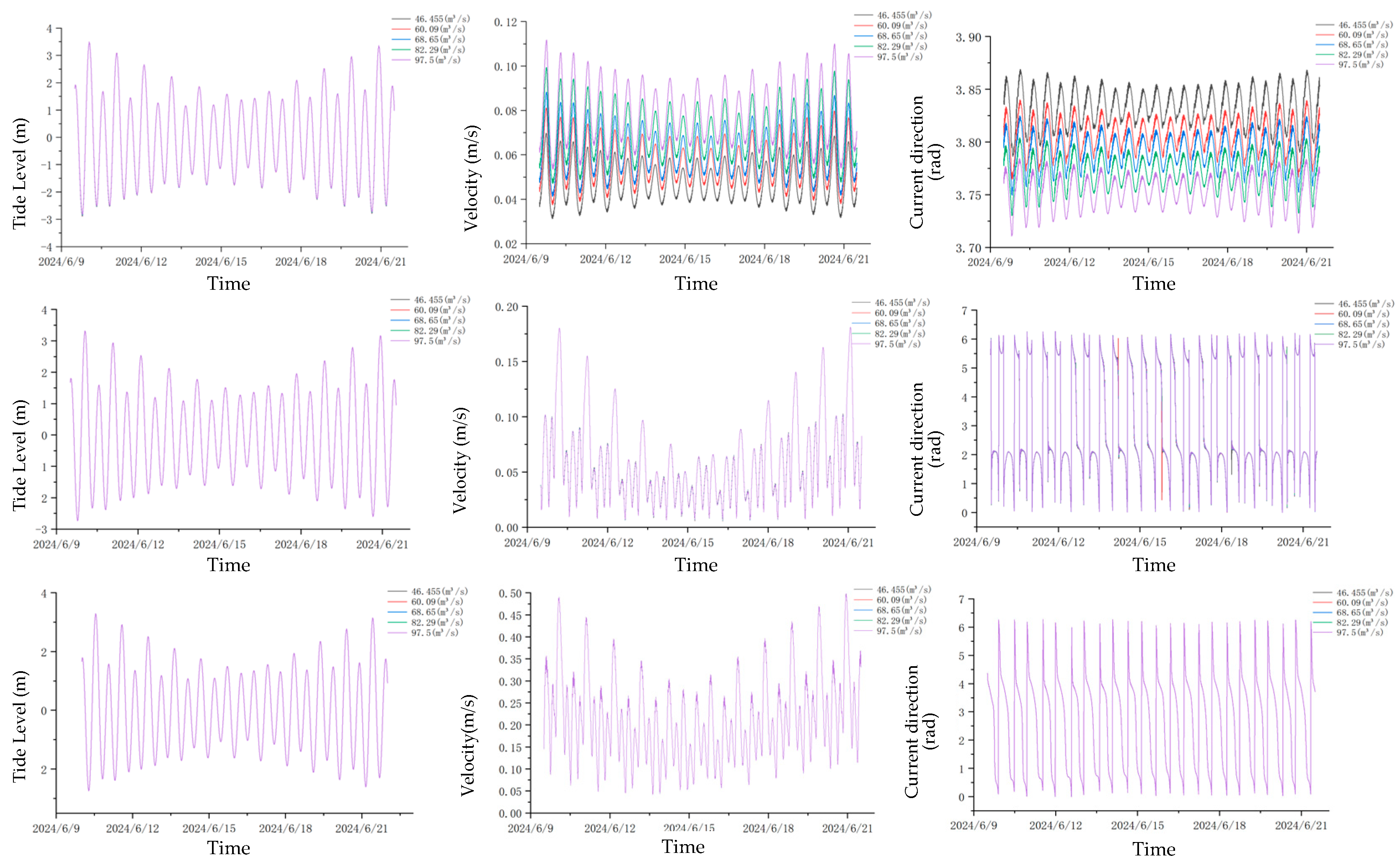
3.3.1. Analysis of Changes in a Hydrodynamic Environment

Figure 11 below shows a comparison of the simulated results of hydrodynamic indicators under five different conditions at three representative locations (3#, 2#, and 1#).

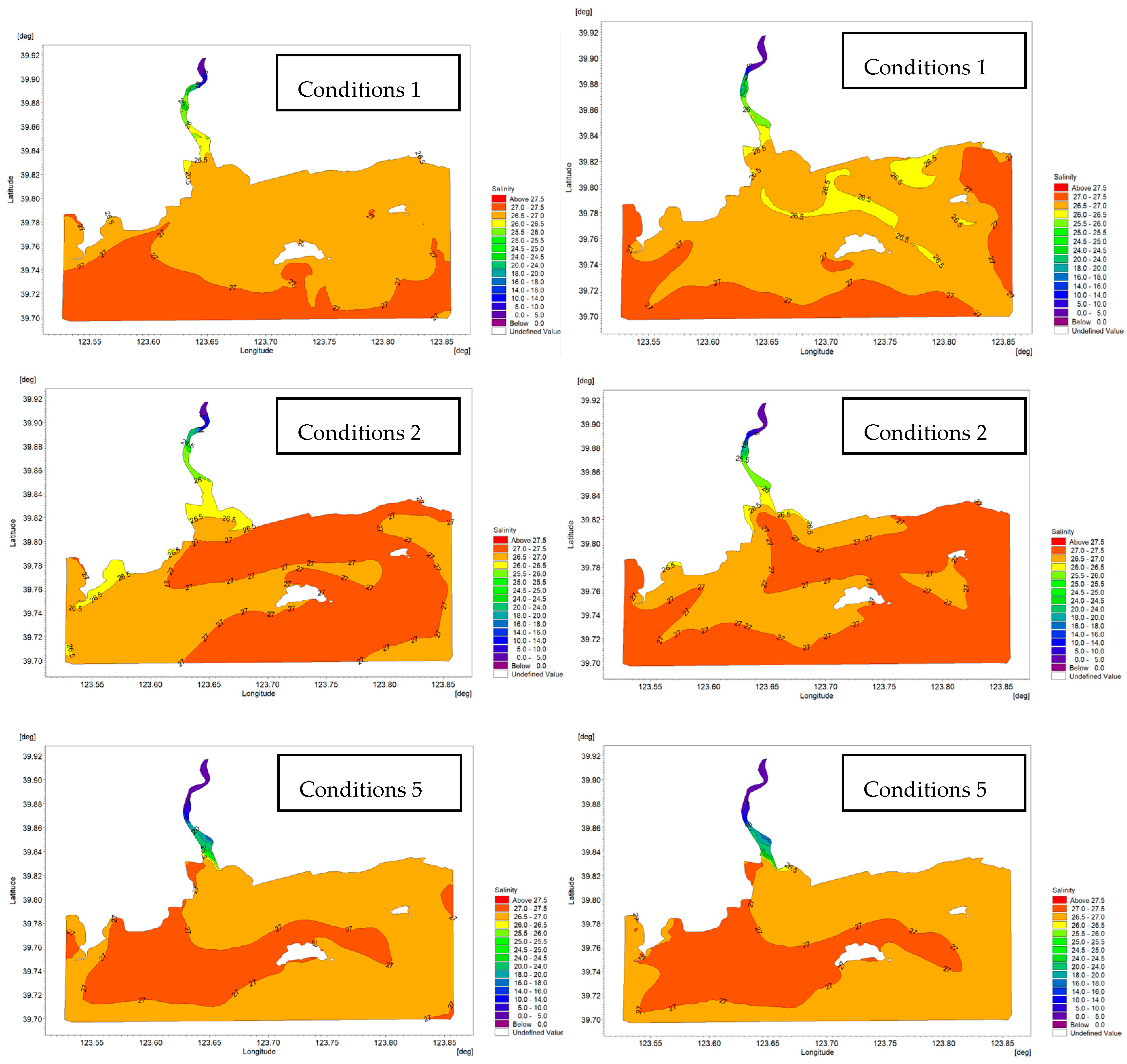
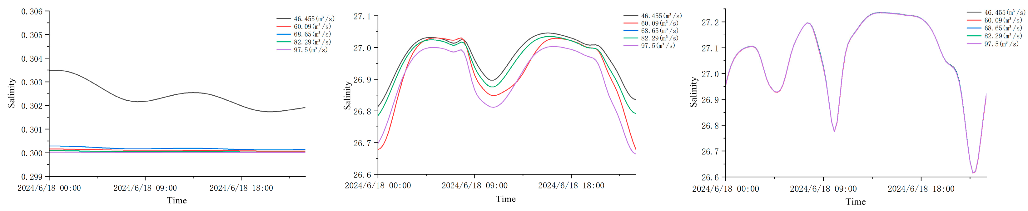
3.3.2. Analysis of Changes in Salinity Distribution

Curve Analysis of Changes in Salinity

Figure 12 shows the results of comparison of salinity values under five different conditions at three representative locations: 3#, 2#, and 1#.

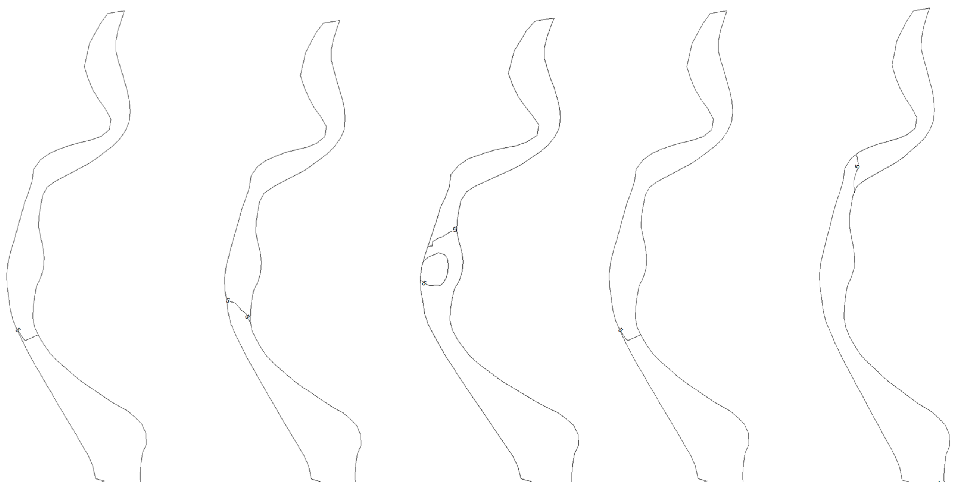
Calculation of Moving Distance of the Isohaline Toward the Estuary

Organisms are more sensitive to a marine hydrological environment with a salinity of 5 [29,30,31]; thus, in order to more clearly express the moving distance of the 5-isohaline before and after water interception, the following figures show a comparison of the movements of the isohaline before and after water interception under various typical schemes, as shown in Figure 13.

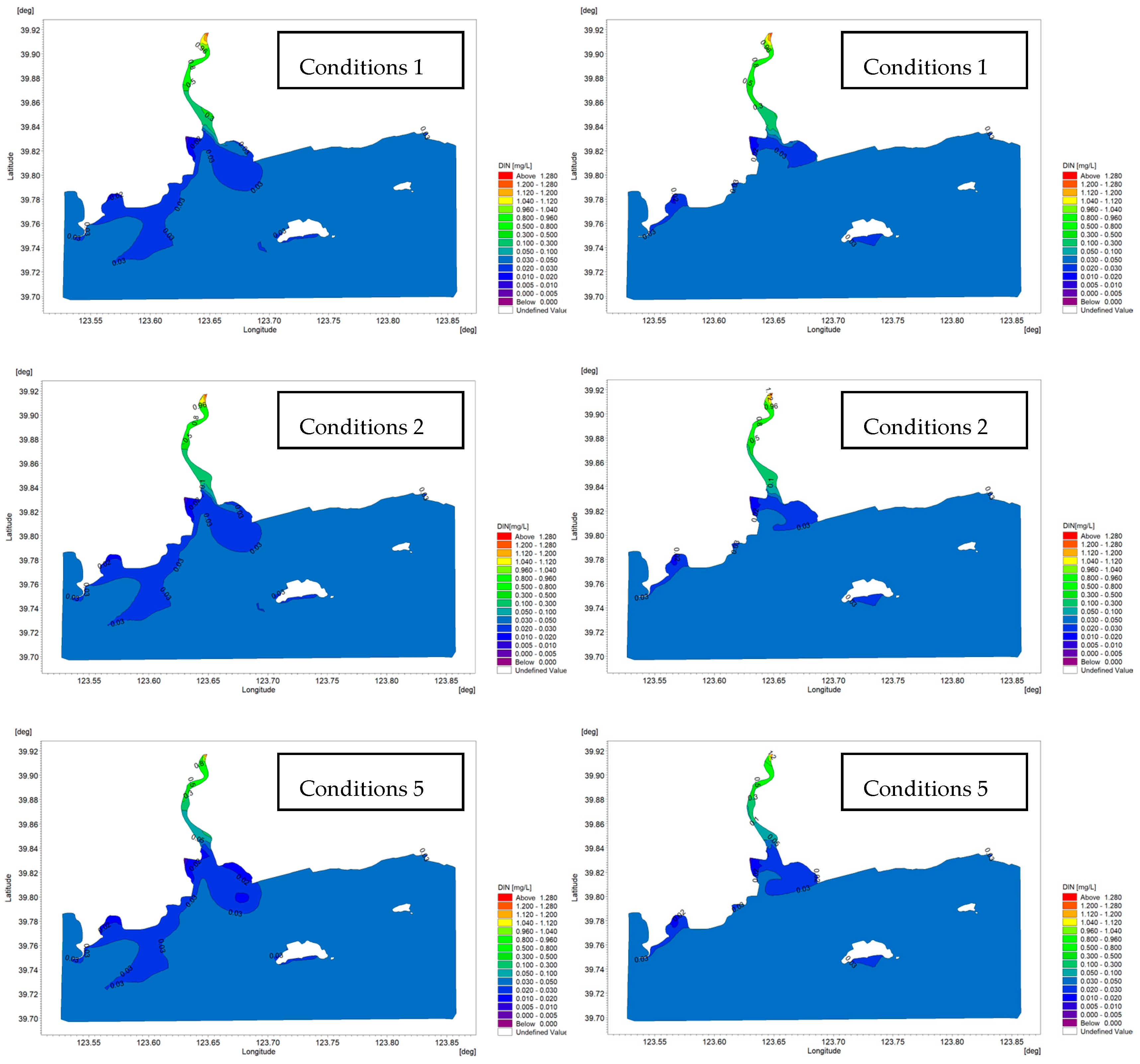
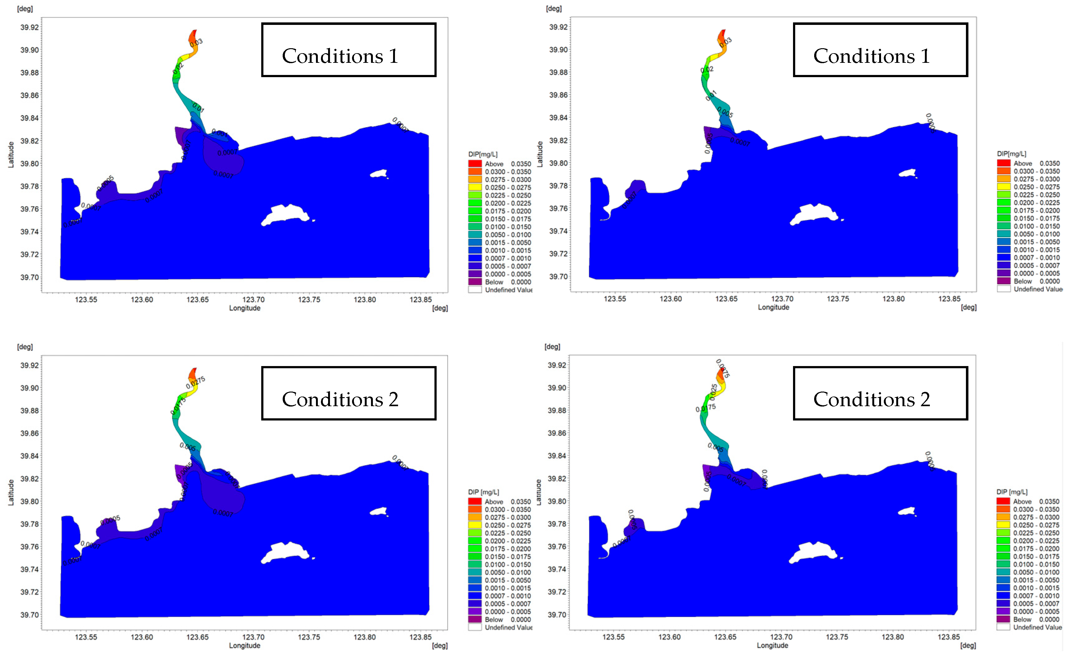
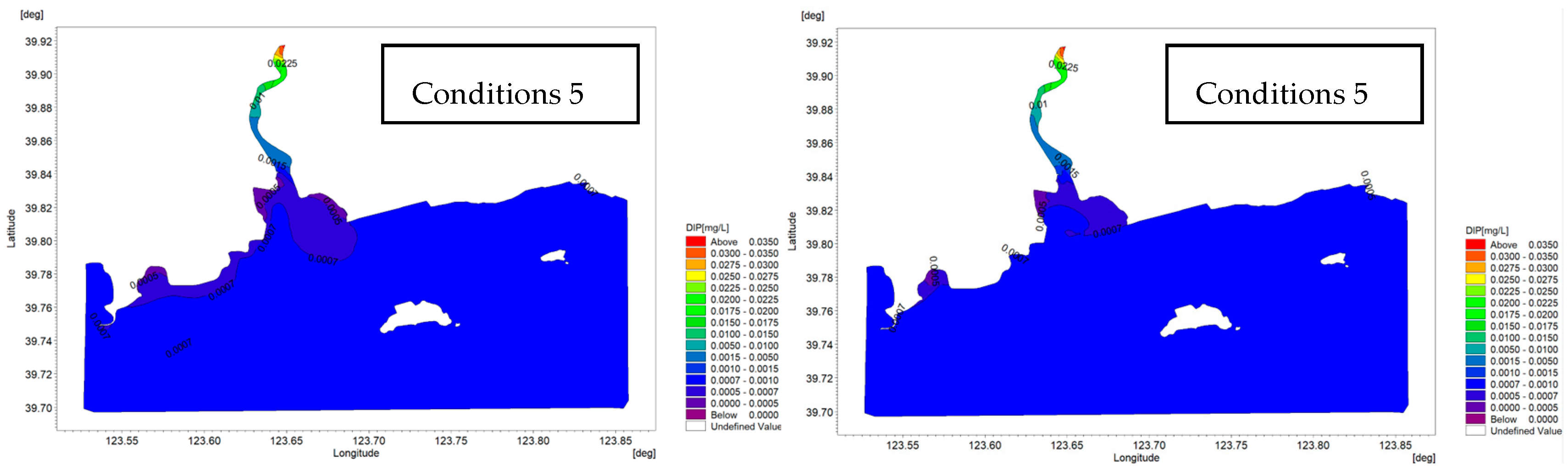
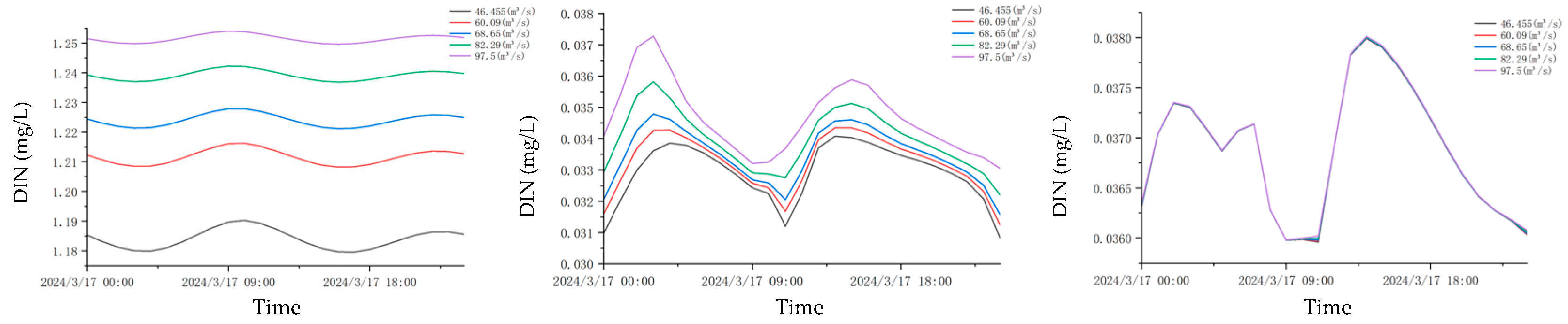
3.3.3. Analysis of Changes in Nutrient Distribution

The time step and calculation accuracy of the water quality module are the same as those of the hydrodynamic model. The nutrient concentrations and a table showing comparison results under different conditions at three representative locations are provided, as shown in the curves in Figure 14 and Figure 15.

4. Discussion

4.1. Changes in Hydrodynamic Conditions Before and After Water Interception

A comparison of the curves for multiple conditions at various stations in the estuary area (as shown in Figure 11) indicates that there was almost no change in tide level under the schemes before and after interception, and the changes in velocity at Stations 2# and 1# were basically negligible. The velocity at Station 3# of the bridge over the river was affected to a certain extent; however, the amount of change in velocity under the current scheme and the scheme with the maximum amount of intercepted water was basically within 10 cm/s, suggesting that there was no obvious change in general. Meanwhile, a comparative analysis of the data collected under the schemes from different stations before and after water interception shows that at a certain station location, with an increase in the amount of intercepted water, the amount of change in hydrodynamic indicators increased accordingly; for different stations involved in this study, as the distance between a station and the estuary increased, the amount of change in velocity decreased.

4.2. Changes in Salinity Distribution Before and After Water Interception

After water interception, due to the reduction of fresh water entering the sea, the salinity of seawater increased to a certain extent. The curve graph (as shown in Figure 12) indicates that at a certain station, the salinity value changed under different interception schemes, and the change at Station 2# in the estuary was the largest with an absolute value of about 0.12. In view of the fact that organisms living in the estuary are more sensitive to a marine hydrological environment with a salinity of 5, in order to describe the changes in the location of the 5-isohaline before and after water interception, the locations of the 5-isohaline under five runoff schemes were simulated sequentially, and its moving distances were calculated based on the scheme before water interception. The results (as shown in Figure 13) indicate that compared with the scheme before water interception, the moving distance of the 5-isohaline to the upper direction of the river channel was 778 m under Scheme 2, 1396 m under Scheme 3, 1735 m under Scheme 4, and 3420 m under Scheme 5 after water interception. Meanwhile, in order to further reflect the importance of salinity to the growth of organisms, changes in the area where salinity was less than 26.8 before and after water interception were analyzed and discussed in this paper. The findings show that with an increase in the interception rate, the amount of reduction of the envelope area gradually increased. At the maximum interception rate, the amount of change is 6.5145 million square meters and the change rate is about 10.7%, which clearly show that water interception for irrigation indeed has a certain impact on salinity distribution in the estuary. A comparison of various schemes shows that when the natural conditions, such as river width and water depth, remain unchanged, the impact increases with an increase in the interception rate. In this paper, the findings show that under the scheme with the maximum interception rate, the longer the moving distance of the 5-isohaline, the greater the amount of change in the area of the envelope curve with a salinity of 26.8.

4.3. Changes in Nutrient Distribution Before and After Water Interception

A comparison of the simulation results (as shown in Figure 14 and Figure 15) indicates that there is a certain change in nutrient contents before and after water interception, but such a change is not significant. The amount of change is related to the amount of intercepted water and the distance between a station and the estuary. Specifically, at a certain station, as interception rate increases, the amount of change in nutrient contents increases. Under the scheme with the maximum interception rate, the content of inorganic nitrogen decreases by up to 5.39%, and the content of inorganic phosphorus decreases by up to 6.34% compared with those under the scheme before water interception. For different stations under the same interception scheme, as a station’s distance from the estuary increases, the amount of change in nutrient contents decreases. For the representative station farthest from the estuary in the sea area, the minimum amount of change in inorganic nitrogen content is merely 0.04%, and the minimum amount of change in inorganic phosphorus content is merely 0.05%.

5. Conclusions

In this paper, numerical simulation was used to quantitatively calculate the impact of changes in the flow of a typical river emptying into the northern Yellow Sea of China on the water environment of the estuary. Based on a vertical average two-dimensional shallow water model, the distribution of water environmental indicators, such as hydrodynamic indicators, salinity, and nutrient contents, under five design schemes with different interception rates was predicted and analyzed. The final verification and findings show that the numerical model proposed in this paper can simulate and predict the hydrodynamic conditions and water quality conditions of the estuary in a great way.

(1)

A comparison of the curves of various stations in the sea area under multiple schemes (as shown in Figure 11, Figure 12, Figure 13, Figure 14 and Figure 15) indicates that the changes in tide level and velocity the five schemes before and after interception are not obvious. Through the simulation of the locations of the 5-isohaline under five runoff schemes and calculation of its moving distances compared to the scheme before interception, it is found that changes in runoff indeed have a certain impact on salinity distribution in the estuary. A comparison of the schemes shows that when natural conditions, such as river width and water depth, remain unchanged, under the five interception schemes, with an increase in the interception rate, the moving distance of the 5-isohaline gradually increases, and the amount of reduction in the area of the envelope curve with a salinity of 26.8 increases. There is a certain change in nutrient contents before and after interception, and the amount of change is also related to the interception rate and the distance of a station from the estuary.

(2)

Studies on the mechanism of the impact of changes in flow rates of typical rivers emptying into the sea under hydrodynamic conditions must attract sufficient attention from aquaculture operators and people engaging in marine environmental protection. The numerical simulation-based research method used in this paper can provide a technical method for accurately predicting the possible impact of river interception for irrigation on estuarine organisms and coastal wetlands, as well as provide estuarine management authorities with data support to help them learn about changes in water environment, ecological environment, etc., within the scope of coastal wetlands belonging to an estuary in an accurate and real-time manner.

(3)

In future studies, we will focus on solving and reducing the impact of changes in runoff of other similar rivers emptying into the sea on water environment across different years and water periods based on numerical simulation methods. We will simulate the impact of high-density cage aquaculture on water environment using non-generalized CFD methods. For example, during ice periods in winter, we may provide quantitative forecasts and early warnings on the amount of changes in water environment indicators, and even try to ensure the stability of water environment indicators by introducing slow-release nutrient fertilizers and externally patented delivery equipment, as well as cooperating with aquaculture operators in ensuring the supply of nutrients required for the growth of organisms. These measures would ensure high yield and quality of organisms [32,33], helping the aquaculture industry pursue sustainable development and providing aquaculture operators with technical support to help them make scientific and effective decisions on aquaculture.

References

1. Sheng, H. The Variations of Water and Sediment Discharge of the Rivers Along the East Coast of Liaodong Peninsula During the Past Millennium: Simulation, Reconstruction and Driving Mechanism Analysis. Master’s Thesis, Nanjing University of China, Nanjing, China, 2018. [Google Scholar]
2. Shrestha, S.; Soden, B.J. Anthropogenic Weakening of the Atmospheric Circulation During the Satellite Era. Geophys. Res. Lett. 2023, 50, e2023GL104784. [Google Scholar] [CrossRef]
3. Nivesh, S.; Patil, J.P.; Goyal, V.C.; Saran, B.; Singh, A.K.; Raizada, A.; Malik, A.; Kuriqi, A. Assessment of future water demand and supply using WEAP model in Dhasan River Basin, Madhya Pradesh, India. Environ. Sci. Pollut. Res. Int. 2023, 30, 27289–27302. [Google Scholar] [CrossRef] [PubMed]
4. Sun, D.; Wang, J.; Fu, Q.; Chen, L.; Chen, J.; Sun, T.; Li, B. Artificial river flow regulation triggered spatio-temporal changes in marine macrobenthos of the Yellow River Estuary. Mar. Environ. Res. 2024, 202, 106804. [Google Scholar] [CrossRef]
5. Rostamzadeh-Renani, M.; Rostamzadeh-Renani, R.; Baghoolizadeh, M. The effect of vortex generators on the hydrodynamic performance of a submarine at a high angle of attack using a multi-objective optimization and computational fluid dynamics. Ocean Eng. 2023, 282, 114932. [Google Scholar] [CrossRef]
6. Gong, W.; Lin, Z.; Zhang, H.; Lin, H. The response of salt intrusion to changes in river discharge, tidal range, and based on wavelet in the Modaomen China. Ocean Coastal Manag. 2022, 219, 106060. [Google Scholar] [CrossRef]
7. Shou, W.; Zong, H.; Ding, P. A numerical study on the impact of the Yellow River runoff emptying into the sea on the circulation in the Yellow River estuary and nearby waters in summer. Acta Oceanolog. Sin. 2016, 38, 1–13. [Google Scholar]
8. Rostamzadeh-Renani, M.; Baghoolizadeh, M.; Sajadi, S.M.; Rostamzadeh-Renani, R.; Azarkhavarani, N.K.; Salahshour, S.; Toghraie, D. A multi-objective and CFD based optimization of roof-flap geometry and position for simultaneous drag and lift reduction. Propuls. Pow. Res. 2024, 13, 26–45. [Google Scholar] [CrossRef]
9. Gao, Z.; Yang, J.; Cui, W.; Zhang, H. Impact of the reduction of the Yellow River runoff emptying into the sea on the estuary and marine ecological environment and countermeasures. In Proceedings of the 2003 China Environmental Resources Law Seminar (Annual Conference), Qingdao, China, 2 July 2003; pp. 314–318. [Google Scholar]
10. Rostamzadeh-renani, M.; Baghoolizadeh, M.; Rostamzadeh-renani, R.; Toghraie, D.; Ahmadi, B. The effect of canard’s optimum geometric design on wake control behind the car using Artificial Neural Network and Genetic Algorithm. ISA Trans. 2022, 131, 427–443. [Google Scholar] [CrossRef]
11. Zhao, G.; Zhang, Z.; Liang, R.; Pu, X.; Li, K.; Wang, Y. Impact of changes in runoff in the Beimenjiang River estuary on the water environment at the estuarine reach. Yangtze River 2018, 49, 6. [Google Scholar]
12. Quang, N.H.; Sasaki, J.; Higa, H.; Huan, N.H. Spatiotemporal Variation of Turbidity Based on Landsat 8 OLI in Cam Ranh Bay and Thuy Trieu Lagoon, Vietnam. Water 2017, 9, 570. [Google Scholar] [CrossRef]
13. Zhu, Y.; Huang, X.; Xie, R.; Wy, C. An experimental study on the effect of runoff rate on saltwater intrusion into an estuary and its application. Chem. Eng. Equip. 2020, 3, 11–13. [Google Scholar]
14. Liang, J.; Xu, Y.; Zhang, W.; Zhou, R. Effect of runoff change of north river and west river on salt Intrusion in tidal estuary. Sci. Technol. Eng. 2024, 24, 2893–2900. [Google Scholar]
15. Gong, Y. A Numerical Simulation-Based Study on the Spatial and Temporal Distribution of Nutrients and Phytoplankton in the Liaohe Estuary; Dalian Ocean University: Dalian, China, 2024. [Google Scholar]
16. Wu, Q. A Simulation-Based Study on The Impact of the Yangtze River Runoff on Phytoplankton in the Yangtze River Estuary; Nanjing University of Information Science and Technology: Nanjing, China, 2021. [Google Scholar]
17. Wang, Y.; Liu, Z.; Zhang, Y.; Wang, M.; Liu, D. Spatial and temporal variation characteristics of chlorophyll a and environmental factors in Jiaozhou Bay from 2010 to 2011. ACTAOceanolog. Sin. 2015, 37, 103–116. [Google Scholar]
18. Shi, F.; Dong, X. Three-dimension numerical simulation for vulcanization process based on unstructured tetrahedron mesh. J. Manuf. Process. 2016, 22, 1–6. [Google Scholar]
19. Zhang, P.; Zhang, R.J.; Huang, J.M.; Sheng, Z.; Wang, S. FVCOM model-based study on tidal prism and water exchange capacity of Haizhou Bay. Water Resour. Hydropower Eng. 2021, 52, 143–151. [Google Scholar]
20. Chen, C.; Liu, H.; Beardsley, R.C. An Unstructured Grid, Finite-Volume, Three-Dimensional, Primitive Equations Ocean Model: Application to Coastal Ocean and Estuaries. J. Atmos. Ocean. Technol. 2003, 20, 159–186. [Google Scholar]
21. Zhao, C.; Ren, L.; Yuan, F.; Zhang, L.; Jiang, S.; Shi, J.; Chen, T.; Liu, S.; Yang, X.; Liu, Y.; et al. Statistical and Hydrological Evaluations of Multiple Satellite Precipitation Products in the Yellow River Source Region of China. Water 2020, 12, 3082. [Google Scholar] [CrossRef]
22. Marino, M.; Faraci, C.; Jensen, B.; Musumeci, R.E. Turbulent features of nearshore wave–current flow. Ocean Sci. 2024, 20, 1479–1493. [Google Scholar]
23. Minhaz, F.A.; Mazlin, B.M.; Chen, K.L.; Nuriah, A.M. Identification of Water Pollution Sources for Better Langat River Basin Management in Malaysia. Water 2022, 14, 1904. [Google Scholar] [CrossRef]
24. Liu, X.; Ma, D.G.; Zhang, Q.H. A higher-efficient non-hydrostatic finite volume model for strong three-dimensional free surface flows and sediment transport. China Ocean. Eng. 2017, 31, 736–746. [Google Scholar]
25. Stanovoy, V.V.; Eremina, T.R.; Isaev, A.V.; Neelov, I.A.; Vankevich, R.E.; Ryabchenko, V.A. Modeling of oil spills in ice conditions in the Gulf of Finland on the basis of an operative forecasting system. Marine Phys. 2012, 52, 754–759. [Google Scholar]
26. Smagorinsky, J. General circulation experiments with the primitive equations: I. The basic experiment. Mon. Weather Rev. 1963, 91, 99–164. [Google Scholar]
27. Wang, K.; Li, N.; Wang, Z.; Song, G.; Du, J.; Song, L.; Jiang, H.; Wu, J. The Impact of Floating Raft Aquaculture on the Hydrodynamic Environment of an Open Sea Area in Liaoning Province, China. Water 2022, 14, 3125. [Google Scholar] [CrossRef]
28. Wang, K.; Li, N.; Song, L.; Jiang, H. Application of a VOF Multiphase Flow Model for Issues concerning Floating Raft Aquaculture. Water 2023, 15, 3450. [Google Scholar] [CrossRef]
29. Wang, Y.; Zhou, W. Research progress on the effect of salinity on pond aquaculture. Jiangsu J. Agric. Sci. 2022, 38, 278–284. [Google Scholar]
30. Qin, H.; Yang, S.; Wang, B.; Liao, X.; Hu, S.; Zhao, J.; He, Z.; Sun, C. Effects of different salinity levels on biological floccules, prawn growth and enzyme activity. Jiangsu J. Agric. Sci. 2020, 39, 400–406. [Google Scholar]
31. Zhang, K. Research on Ph and Salinity Control Technology Fora Culture Environment for Biological Floccules of Prawns; Ocean University of China: Qingdao, China, 2015. [Google Scholar]
32. Li, L.; Wu, L.; Yuan, J.; Zhao, X.; Xia, Y. Water Environment in Macro-Tidal Muddy Sanmen Bay. J. Mar. Sci. Eng. 2025, 13, 55. [Google Scholar]
33. Al-Mur, B.A. Environmental Assessment Using Phytoplankton Diversity, Nutrients, Chlorophyll-a, and Trophic Status Along Southern Coast of Jeddah, Red Sea. J. Mar. Sci. Eng. 2025, 13, 29. [Google Scholar]
Figure 1. Location and scope of the estuary involved in the study.
Jmse 13 00736 g001
Figure 2. Locations of observation stations.
Jmse 13 00736 g002
Figure 3. Computational domain, topography, and mesh distribution.
Jmse 13 00736 g003
Figure 4. Tide level verification diagram from Station T1.
Jmse 13 00736 g004
Figure 5. Verification of velocitys and directions at the three observation stations.
Jmse 13 00736 g005
Figure 6. Comparison of measured and simulated temperature as well as salinity values at Station P1.
Jmse 13 00736 g006
Figure 7. Flow field simulation results at the times of rapid fall (left) and rapid rise (right) during a spring tide under three typical conditions (Conditions 1, 2, and 5).
Jmse 13 00736 g007aJmse 13 00736 g007b
Figure 8. Salinity field simulation results at the times of rapid fall (left) and rapid rise (right) during a spring tide under three typical conditions (Conditions 1, 2, and 5).
Jmse 13 00736 g008
Figure 9. Distribution of the inorganic nitrogen concentration field at the times of rapid fall (left) and rapid rise (right) during a spring tide under three typical conditions (Conditions 1, 2, and 5).
Jmse 13 00736 g009
Figure 10. Distribution of the inorganic phosphorus concentration field at the times of rapid fall (left) and rapid rise (right) during a spring tide under three typical conditions (Conditions 1, 2, and 5).
Jmse 13 00736 g010aJmse 13 00736 g010b
Figure 11. Comparison of simulated values of hydrodynamic indicators (tide level, velocity, and current direction) under different conditions at three representative locations.
Jmse 13 00736 g011
Figure 12. Comparison of simulated salinity values under different conditions at three characteristic representative locations.
Jmse 13 00736 g012
Figure 13. Comparison of movements of the 5-isohaline under Condition 1 before interception and Conditions 2, 3, 4, and 5 after interception.
Jmse 13 00736 g013
Figure 14. Comparison of simulated values of inorganic nitrogen under different conditions at three characteristic representative locations.
Jmse 13 00736 g014
Figure 15. Comparison of simulated values of inorganic phosphorus under different working conditions at three characteristic representative locations.
Jmse 13 00736 g015