
Merging Multiple System Perspectives: The Key to Effective Inland Shipping Emission-Reduction Policy Design


Abstract
1. Introduction
2. Materials and Methods
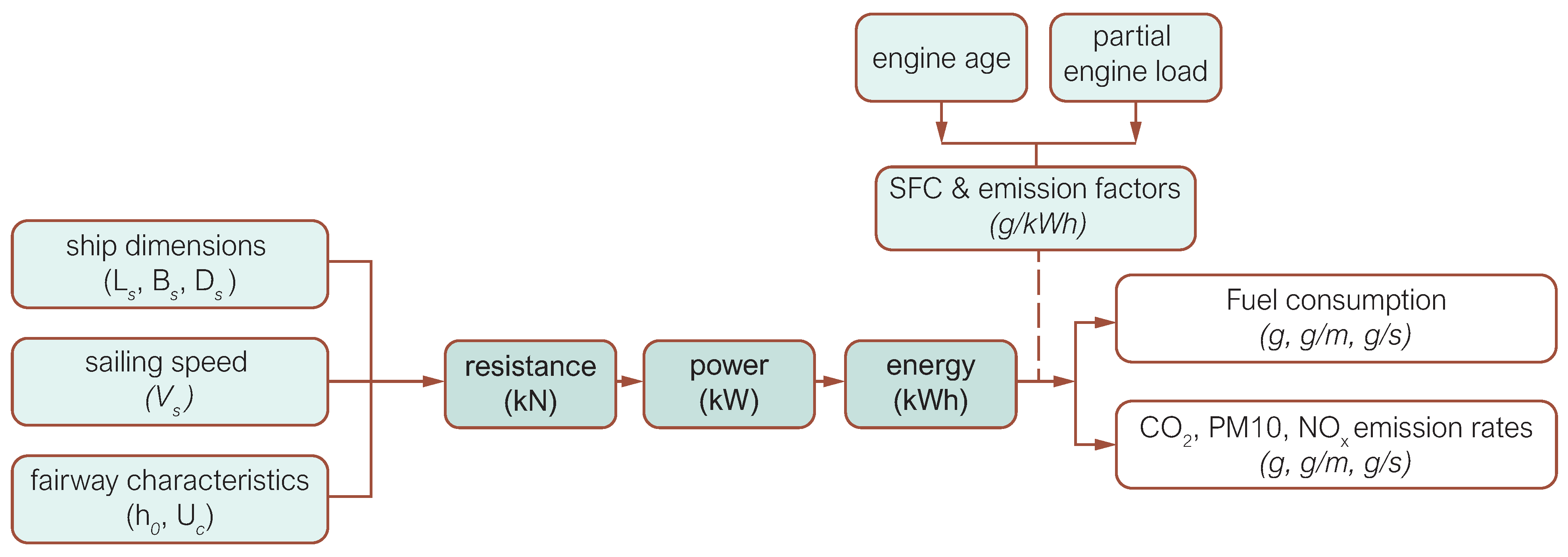
2.1. Emission Estimation Method
2.2. Data Sources
- AIS data
- CEMT classification
- Engine age distribution
- FIS data
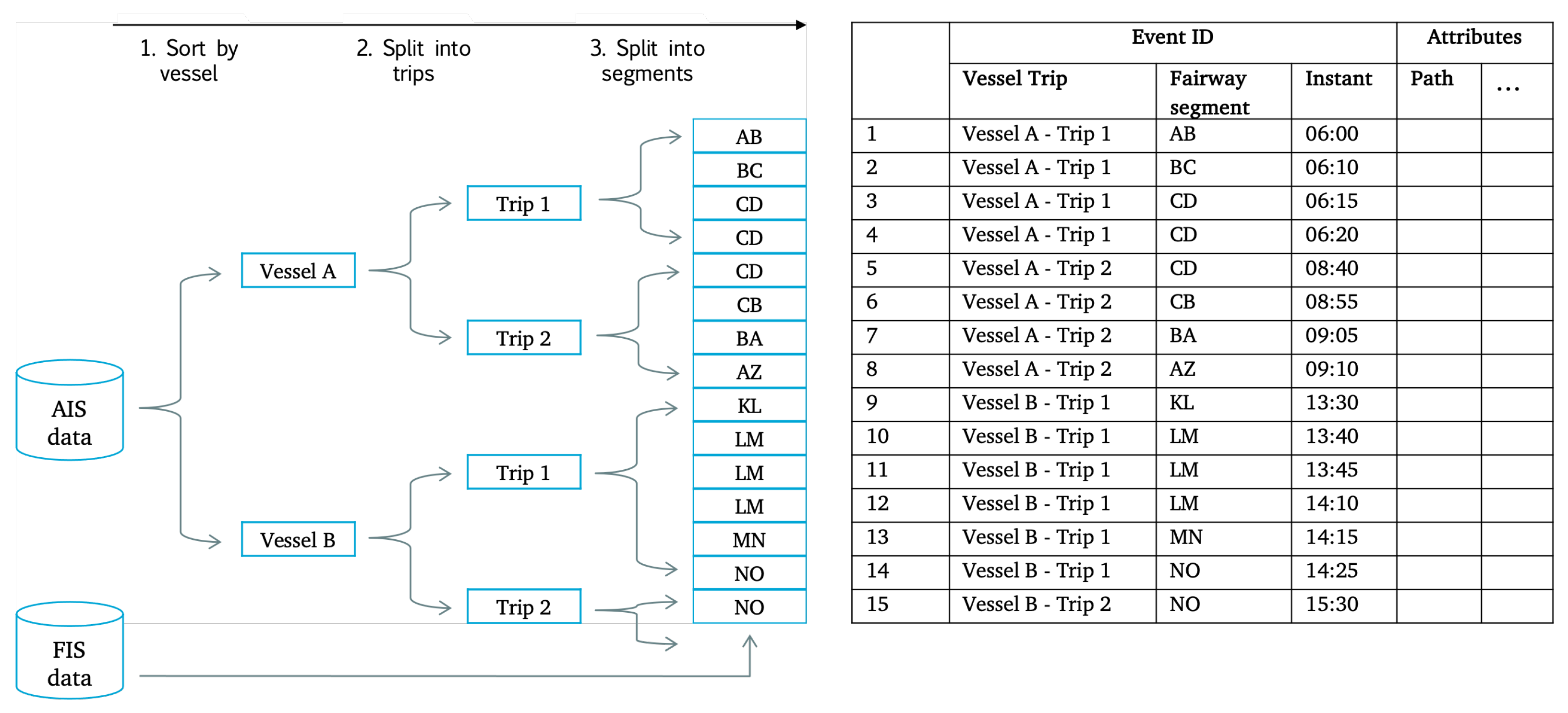
2.3. Designing the Event Table: A Concept for Multi-Perspective Emission Evaluation

| Perspective | Requirement | |
|---|---|---|
| Scales—The ‘where’ and ‘when’ of the performance, uncovering spatial patterns and temporal variations | Fundamental components | The highest level of detail in time (seconds, hours, months, etc.) The highest level of detail in space (meters, street/city/country level, etc.) |
| Aggregation means | For deriving time aggregates (hours, days, weeks, months, etc.) For deriving spatial aggregates (street, river, area, state, etc.) | |
| Conditions—Understand how system performance is connected to its underlying processes and their environment | Fundamental components | The highest level of detail of environmental and process description |
| Influencing factors | Attributes that indicate influencing factors, and that couple them to performance | |
| Behavior—How the performance of the system is influenced by the behavior of individual agents or collectives | Fundamental components | The highest detail level of individual agent or process to keep track of |
| Activity sequence | Means to track the sequence of activities performed by the agent | |
| Dependencies—Identify causal relationships, critical paths, and sensitivities within the entire system | Initiations | Dependency of an event on (an)other event(s) |
| Perspective | Requirement | |
|---|---|---|
| Scales—Spatial patterns of inland shipping emissions including hotspots | Fundamental components | Seconds Fairway segment |
| Aggregation means | Fairway graph | |
| Conditions—The influence of the environmental conditions on the emissions | Influencing factors | Water depth, current speed, vessel properties |
| Coupling factors | Intermediate calculation outcomes | |
| Behavior—Understand how vessel behavior contributes to the emissions | Agent identity | Vessel identity, trip and activity (sailing or pausing) |
| Activity sequence | Time stamps | |
| Dependencies—Not considered | Initiations | - |
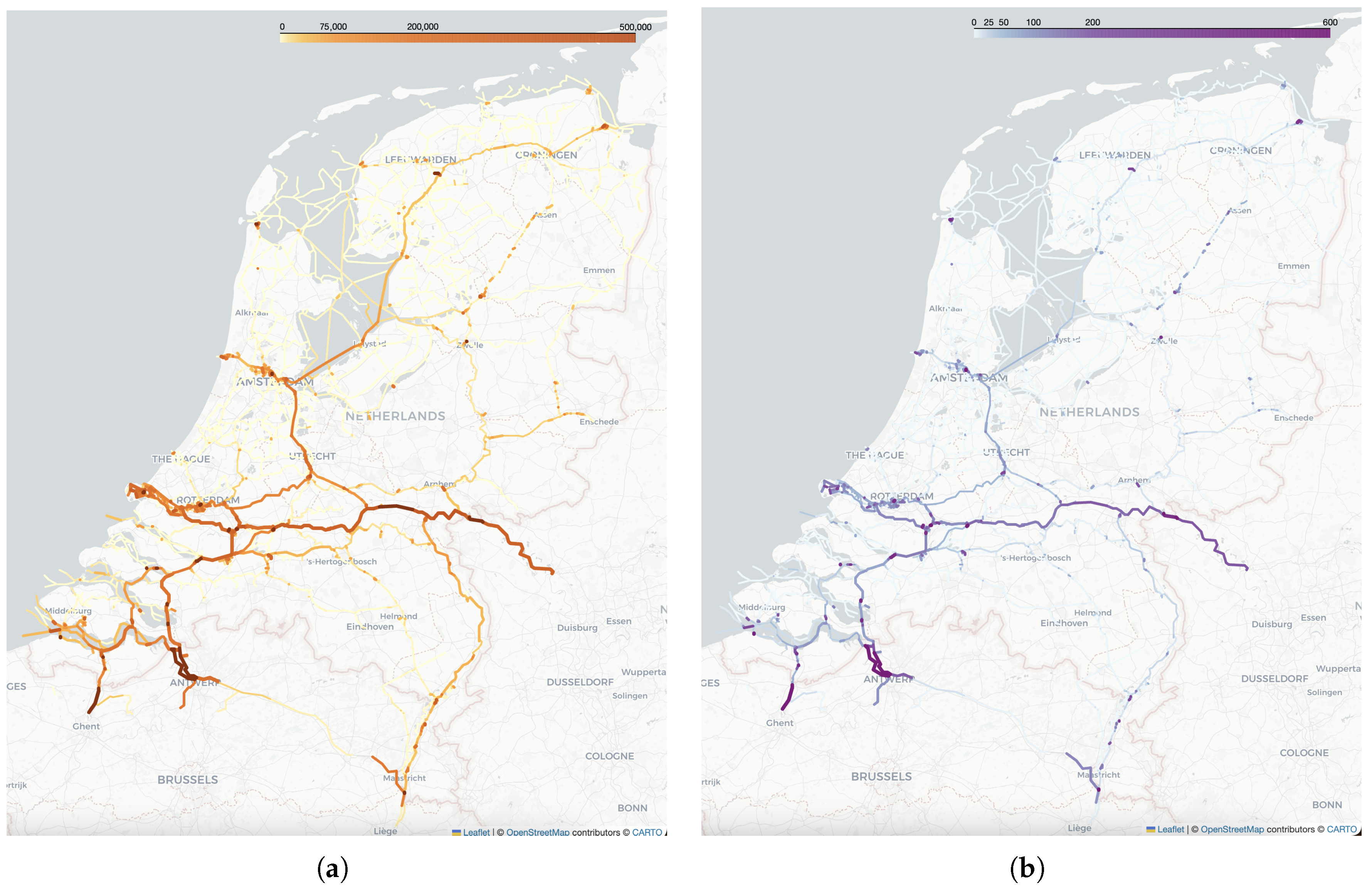
- Scales
- Conditions
- Behavior
- Dependencies
2.4. Computing Event-Based Inland Shipping Emissions
3. Results
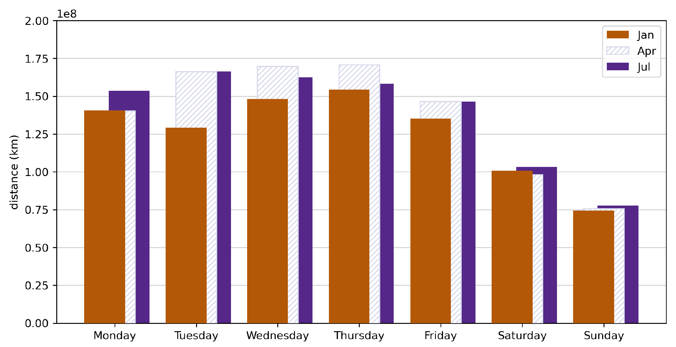
- Scales
- Conditions
- Behavior
4. Discussion
4.1. Contribution to Emission-Reduction Policy Design
4.2. Discussion of the Limitations and Future Work
5. Conclusions
Author Contributions
Funding
Data Availability Statement
Acknowledgments
Conflicts of Interest
Abbreviations
| AIS | Automatic Identification System |
| CEMT | Conférence Européenne des Minstres de Transports |
| FIS | Fairway Information System |
| GSC | Green Shipping Corridor |
| IMO | International Maritime Organisation |
| LNG | Liquefied Natural Gas |
| SFC | Specific Fuel Consumption |
| SOG | Speed Over Ground |
| STW | Speed Through Water |
Appendix A. Vessel Energy Use Calculation
References
- United Nations/Framework Convention on Climate Change. Adoption of the Paris Agreement. In Proceedings of the 21st Conference of the Parties, Paris, France, 12 December 2015; United Nations: New York, NY, USA, 2015. Ch. UNTC XXVII 7.d. [Google Scholar]
- European Commission. The European Green Deal. Bill. 2019. Available online: https://commission.europa.eu/strategy-and-policy/priorities-2019-2024/european-green-deal_en (accessed on 4 March 2025).
- Marine Environment Protection Committee. RESOLUTION MEPC.304(72)—Adoption of the Initial IMO Strategy on Reduction of GHG Emissions from Ships; Resolution; Marine Environment Protection Committee: London, UK, 2018. [Google Scholar]
- Dutch Inland Shipping Green Deal. Green Deal on Maritime and Inland Shipping and Ports. Bill, The Hague. 2019. Available online: https://www.greendeals.nl/sites/default/files/2019-11/GD230%20Greenf%20Deal%20on%20Maritime%20and%20Inland%20shipping%20and%20Ports.pdf (accessed on 4 March 2025).
- Minister of Infrastructure and Water Management. Subsidieverlening Zero Emission Services, Aanleg Laadstations en Aanschaf Energiecontainers; Decree; Minister of Infrastructure and Water Management: The Hague, The Netherlands, 2022. [Google Scholar]
- Song, Z.-Y.; Prem Chhetri, G.Y.; Lee, P.T.W. Green maritime logistics coalition by green shipping corridors: A new paradigm for the decarbonisation of the maritime industry. Int. J. Logist. Res. Appl. 2023, 28, 363–379. [Google Scholar] [CrossRef]
- Port of Rotterdam. Partners Launch Condor H2 for Emission-Free Inland and Near-Shore Shipping. 2023. Available online: https://www.portofrotterdam.com/en/news-and-press-releases/whs2023-partners-launch-condor-h2-for-emission-free-inland-and-near-shore (accessed on 20 June 2024).
- Luo, X.; Yan, R.; Wang, S. Ship sailing speed optimization considering dynamic meteorological conditions. Transp. Res. Part C Emerg. Technol. 2024, 167, 104827. [Google Scholar] [CrossRef]
- Jiang, H.; Peng, D.; Wang, Y.; Fu, M. Comparison of inland ship emission results from a real-world test and an ais-based model. Atmosphere 2021, 12, 1611. [Google Scholar] [CrossRef]
- Kurtenbach, R.; Vaupel, K.; Kleffmann, J.; Klenk, U.; Schmidt, E.; Wiesen, P. Emissions of NO, NO2 and PM from inland shipping. Atmos. Chem. Phys. 2016, 16, 14285–14295. [Google Scholar] [CrossRef]
- Eger, P.; Mathes, T.; Zavarsky, A.; Duester, L. Measurement report: Inland ship emissions and their contribution to NOx and ultrafine particle concentrations at the Rhine. Atmos. Chem. Phys. 2023, 23, 8769–8788. [Google Scholar] [CrossRef]
- Krause, K.; Wittrock, F.; Richter, A.; Busch, D.; Bergen, A.; Burrows, J.P.; Freitag, S.; Halbherr, O. Determination of NOx emission rates of inland ships from onshore measurements. Atmos. Meas. Tech. 2023, 16, 1767–1787. [Google Scholar] [CrossRef]
- Keuken, M.P.; Moerman, M.; Jonkers, J.; Hulskotte, J.; van der Gon, H.A.D.; Hoek, G.; Sokhi, R.S. Impact of inland shipping emissions on elemental carbon concentrations near waterways in The Netherlands. Atmos. Environ. 2014, 95, 1–9. [Google Scholar] [CrossRef]
- PIANC InCom. WG234 Infrastructure for the Decarbonisation of IWT; Report, PIANC-InCom-WG234; PIANC InCom: Brussels, Belgium, 2023. [Google Scholar]
- Fan, A.; Wang, J.; He, Y.; Perčić, M.; Vladimir, N.; Yang, L. Decarbonising inland ship power system: Alternative solution and assessment method. Energy 2021, 226, 120266. [Google Scholar] [CrossRef]
- Evers, V.; Kirkels, A.; Godjevac, M. Carbon footprint of hydrogen-powered inland shipping: Impacts and hotspots. Renew. Sustain. Energy Rev. 2023, 185, 113629. [Google Scholar] [CrossRef]
- Fan, A.; Xiong, Y.; Yang, L.; Zhang, H.; He, Y. Carbon footprint model and low–carbon pathway of inland shipping based on micro–macro analysis. Energy 2023, 263, 126150. [Google Scholar] [CrossRef]
- Tan, Z.; Zeng, X.; Shao, S.; Chen, J.; Wang, H. Scrubber installation and green fuel for inland river ships with non-identical streamflow. Transp. Res. Part E Logist. Transp. Rev. 2022, 161, 102677. [Google Scholar] [CrossRef]
- Gao, D.; Zhang, W.; Shen, A.; Wang, Y. Parameter design and energy control of the power train in a hybrid electric boat. Energies 2017, 10, 1028. [Google Scholar] [CrossRef]
- Zhang, Y.; Sun, L.; Fan, T.; Ma, F.; Xiong, Y. Speed and energy optimization method for the inland all-electric ship in battery-swapping mode. Ocean Eng. 2023, 284, 115234. [Google Scholar] [CrossRef]
- Ahamad, N.B.B.; Guerrero, J.M.; Su, C.L.; Vasquez, J.C.; Zhaoxia, X. Microgrids Technologies in Future Seaports. In Proceedings of the 2018 IEEE International Conference on Environment and Electrical Engineering and 2018 IEEE Industrial and Commercial Power Systems Europe (EEEIC/I&CPS Europe), Palermo, Italy, 12–15 June 2018; pp. 1–6. [Google Scholar] [CrossRef]
- Jiang, M.; Baart, F.; Visser, K.; Hekkenberg, R.; Van Koningsveld, M. Corridor Scale Planning of Bunker Infrastructure for Zero-Emission Energy Sources in Inland Waterway Transport. In Proceedings of PIANC Smart Rivers 2022; Li, Y., Hu, Y., Rigo, P., Lefler, F.E., Zhao, G., Eds.; Springer Nature: Singapore, 2023; pp. 334–345. [Google Scholar] [CrossRef]
- Šimenc, M. Overview and comparative analysis of emission calculators for inland shipping. Int. J. Sustain. Transp. 2016, 10, 627–637. [Google Scholar] [CrossRef]
- Goldsworthy, L.; Goldsworthy, B. Modelling of ship engine exhaust emissions in ports and extensive coastal waters based on terrestrial AIS data—An Australian case study. Environ. Model. Softw. 2015, 63, 45–60. [Google Scholar] [CrossRef]
- Jalkanen, J.P.; Johansson, L.; Kukkonen, J.; Brink, A.; Kalli, J.; Stipa, T. Extension of an assessment model of ship traffic exhaust emissions for particulate matter and carbon monoxide. Atmos. Chem. Phys. 2012, 12, 2641–2659. [Google Scholar] [CrossRef]
- PIANC InCom. Guideline for Air Pollutants and Carbon Emissions Performance Indicators for Inland Waterways; Report, PIANC-InCom-WG229; PIANC InCom: Brussels, Belgium, 2024. [Google Scholar]
- Jiang, M.; Segers, L.; van der Werff, S.; Baart, F.; van Koningsveld, M. OpenTNSim, Version v1.1.1; Zenodo: Geneva, Switzerland, 2022. [CrossRef]
- Segers, L. Mapping Inland Shipping Emissions in Time and Space for the Benefit of Emission Policy Development. Master’s Thesis, Delft University of Technology, Delft, The Netherlands, 2021. [Google Scholar]
- van Koningsveld, M.; van der Werff, S.; Jiang, M.; Lansen, J.; de Vriend, H. Ports and Waterways—Navigating the Changing World; Chapter Performance of Ports and Waterway Systems; TU Delft Open: Delft, The Netherlands, 2021; pp. 433–458. [Google Scholar] [CrossRef]
- Holtrop, J.; Mennen, G. A statistical Power Prediction Method. Int. Shipbuild. Prog. 1978, 25, 253–256. [Google Scholar]
- Terwisga, T. Weerstand en Voortstuwing van Bakken: Een Literatuurstudie; Technical Report 49199-1-RD; Maritiem Research Instituut Nederland: Wageningen, The Netherlands, 1989. [Google Scholar]
- Zeng, Q.; Thill, C.; Hekkenberg, R.; Rotteveel, E. A modification of the ITTC57 correlation line for shallow water. J. Mar. Sci. Technol. 2019, 24, 642–657. [Google Scholar] [CrossRef]
- Hofman, M.; Kozarski, V. Shallow Water Resistance Charts for Preliminary Vessel Design. Int. Shipbuild. Prog. 2000, 47, 61–76. [Google Scholar]
- Hekkenberg, R.G. Inland Ships for Efficient Transport Chains. Ph.D. Thesis, Delft University of Technology, Delft, The Netherlands, 2013. [Google Scholar] [CrossRef]
- Ligterink, N.; van Gijswijk, R.; Kadijk, G.; Vermeulen, R.; Indrajuana, A.; Elstgeest, M. Emissiefactoren Wegverkeer—Actualisatie 2019; Technical Report 2019-STL-RAP-100321751; TNO: Den Haag, The Netherlands, 2019. [Google Scholar]
- Maritime Safety Committee. RESOLUTION MSC.74(69); Resolution; Maritime Safety Committee: London, UK, 1998. [Google Scholar]
- Conférence Européenne des Ministres des Transports. Resolution No. 92/2 on New Classification of Inland Waterways; Statute; Conférence Européenne des Ministres des Transports: Bruxelles, Belgium, 1992. [Google Scholar]
- de Jong, J.; Baart, F.; Zagonjolli, M. Topological Network of the Dutch Fairway Information System, Version v0.2.0; Zenodo: Geneva, Switzerland, 2021. [CrossRef]
- Rijkswaterstaat. Fairways and Infrastructure Netherlands. 2024. Available online: https://www.vaarweginformatie.nl (accessed on 20 June 2024).
- van der Werff, S.; van Gelder, P.; Baart, F.; van Koningsveld, M. How Early Integration of Multiple Analysis Perspectives Can Enhance the Understanding of Complex Systems. 2025; in preparation. [Google Scholar] [CrossRef]
- Asahara, A.; Hayashi, H.; Ishimaru, N.; Shibasaki, R.; Kanasugi, H. International Standard “OGC Moving Features” to address “4Vs” on locational BigData. In Proceedings of the 2015 IEEE International Conference on Big Data (Big Data), Santa Clara, CA, USA, 29 October–1 November 2015; pp. 1958–1966. [Google Scholar]
- van der Aalst, W. Process Mining. ACM Trans. Manag. Inf. Syst. 2012, 3, 2. [Google Scholar] [CrossRef]
- Smyth, D.; Checkland, P. Using a Systems Approach: The Structure of Root Definitions. J. Appl. Syst. Anal. 1976, 5, 75–83. [Google Scholar]
- Bunge, M.A. Treatise on Basic Philosophy: Ontology II: A World of Systems; Reidel Publishing Company: Dordrecht, The Netherlands, 1979. [Google Scholar]
- Lukyanenko, R.; Storey, V.C.; Pastor, O. System: A core conceptual modeling construct for capturing complexity. Data Knowl. Eng. 2022, 141, 102062. [Google Scholar] [CrossRef]
- Andrienko, N.; Andrienko, G. Article Visual analytics of movement: An overview of methods, tools and procedures. Inf. Vis. 2013, 12, 3–24. [Google Scholar] [CrossRef]
- Microsoft Open Source; McFarland, M.; Emanuele, R.; Morris, D.; Augspurger, T. microsoft/PlanetaryComputer: October 2022, Version 2022.10.28; Zenodo: Geneva, Switzerland, 2022. [CrossRef]
- Rijkswaterstaat. Richtlijnen Vaarwegen 2020; Rijkswaterstaat Water, Verkeer en Leefomgeving: Rijswijk, The Netherlands, 2020. [Google Scholar]


| Global | Targeted | |
|---|---|---|
| Regulations | Fuel composition (EU regulations RED-III and ETS-2) | Local air quality requirements (municipalities, port authorities) |
| Subsidies | Engine renewal (compliant with latest emission standards) | Zero-emission shipping concepts, Alternative fuel corridors |
| Operational | Speed limits, water management implementation | Optimizing lock operations, providing shore power |
Disclaimer/Publisher’s Note: The statements, opinions and data contained in all publications are solely those of the individual author(s) and contributor(s) and not of MDPI and/or the editor(s). MDPI and/or the editor(s) disclaim responsibility for any injury to people or property resulting from any ideas, methods, instructions or products referred to in the content. |
© 2025 by the authors. Licensee MDPI, Basel, Switzerland. This article is an open access article distributed under the terms and conditions of the Creative Commons Attribution (CC BY) license (https://creativecommons.org/licenses/by/4.0/).
Share and Cite
van der Werff, S.; Baart, F.; van Koningsveld, M. Merging Multiple System Perspectives: The Key to Effective Inland Shipping Emission-Reduction Policy Design. J. Mar. Sci. Eng. 2025, 13, 716. https://doi.org/10.3390/jmse13040716
van der Werff S, Baart F, van Koningsveld M. Merging Multiple System Perspectives: The Key to Effective Inland Shipping Emission-Reduction Policy Design. Journal of Marine Science and Engineering. 2025; 13(4):716. https://doi.org/10.3390/jmse13040716
Chicago/Turabian Stylevan der Werff, Solange, Fedor Baart, and Mark van Koningsveld. 2025. "Merging Multiple System Perspectives: The Key to Effective Inland Shipping Emission-Reduction Policy Design" Journal of Marine Science and Engineering 13, no. 4: 716. https://doi.org/10.3390/jmse13040716
APA Stylevan der Werff, S., Baart, F., & van Koningsveld, M. (2025). Merging Multiple System Perspectives: The Key to Effective Inland Shipping Emission-Reduction Policy Design. Journal of Marine Science and Engineering, 13(4), 716. https://doi.org/10.3390/jmse13040716