A Data-Driven Approach to Analyzing Fuel-Switching Behavior and Predictive Modeling of Liquefied Natural Gas and Low Sulfur Fuel Oil Consumption in Dual-Fuel Vessels

Abstract

International shipping is responsible for approximately 2.7% of the global greenhouse gas emissions, a share expected to rise by as much as 250% by 2050. In response, the International Maritime Organization (IMO) has set ambitious targets to reduce these emissions to near-zero by 2050, focusing on alternative fuels like LNG. This study examines the energy consumption patterns of dual-fuel engines powered by LNG and develops machine learning models using LightGBM to predict fuel usage for both fuel oil (FO) and gas (GAS) modes. The methodology involved analyzing operational data to identify patterns in fuel usage across different voyage conditions. The FO mode was found to be predominantly used for rapid propulsion during speed changes or directional shifts, while the GAS mode was optimized for stable conditions to maximize fuel efficiency. Additionally, a mixed mode of FO and GAS was occasionally applied on complex routes to balance safety and efficiency. Using these insights, LightGBM models were trained to predict fuel consumption in each mode, achieving high accuracy with R² scores of 0.94 for the GAS mode and 0.98 for the FO mode. This model enables ship operators to optimize fuel decisions in response to varying voyage conditions, resulting in reduced overall fuel consumption and lower CO₂ emissions. By applying the predictive model, operators can adjust fuel usage strategies to match operational demands, potentially achieving notable cost savings and meeting stricter environmental regulations. Furthermore, the accurate estimation of fuel usage supports CO₂ emissions management, aligning with the Carbon Intensity Indicator (CII) and providing ship operators with actionable data for fleet management optimization. This research provides essential data to support carbon emission compliance, improves fuel efficiency, and offers practical insights into fuel management strategies. The predictive model serves as a valuable resource for ship operators to optimize fuel use and aligns with the IMO’s environmental targets, aiding the maritime industry’s transition toward carbon neutrality.

1. Introduction

1.1. Background of Study

The issue of carbon neutrality has become a critical global priority in addressing climate change and reducing greenhouse gas emissions. The Paris Agreement, established to limit global warming to well below 2 °C, underscores the importance of achieving carbon neutrality by mid-century. To meet these targets, significant societal transformations and emission reductions across all sectors are essential [1]. The urgency of this transition is further highlighted by the continuous rise in global CO₂ emissions, which reached a record high of 43.1 Gt CO₂ in 2019. Major emitting countries such as the European Union (EU), United States of America (USA), Japan, and Australia have made ambitious commitments to peak CO₂ emissions and achieve carbon neutrality by 2050, necessitating deep and comprehensive changes in energy consumption, industrial processes, and societal behaviors [2]. In the context of global efforts, the EU has played a significant role in promoting carbon neutrality, focusing on substantial emission reductions across its member states through technological and policy reforms. These changes are being applied comprehensively across various sectors, including the shipping industry [1,2,3].

International shipping is currently responsible for about 2.7% of the total global greenhouse gas (GHG) emissions based on data from 2009 [4]. The share of shipping emissions in global anthropogenic emissions has increased from 2.76% in 2012 to 2.89% in 2018 [5]. While this may seem like a small proportion of the global GHG emissions, under a new voyage-based allocation of international shipping, CO₂ emissions have also increased over this same period from 701 million tons in 2012 to 740 million tons in 2018 (5.6% increase) [5]. Furthermore, the overall volume of global maritime trade is increasing, and the trend towards larger ships continues [6]. In 2022, capacity expanded at an annual rate of 3.2 per cent with overall tonnage hitting 2.27 billion dead weight tons. On average, the global fleet was two years older in 2023 compared to a decade earlier [7]. Furthermore, maritime CO₂ emissions are projected to increase significantly in the coming decades. Depending on future economic and energy developments, business-as-usual (BAU) scenarios project an increase of 50% to 250% by 2050 [8]. Therefore, implementing operational measures such as speed limitations, improved fuel efficiency, and the use of cleaner fuels like LNG can significantly reduce emissions in the short to medium term. For instance, introducing speed restriction zones and onshore power supply systems can reduce NOx and CO₂ emissions by up to 15% [9]. Furthermore, mitigation strategies involving the integration of carbon capture technologies onboard ships are being explored as a means to achieve long-term emission reductions [10]. In summary, responding to environmental changes necessitates the adoption of market-based strategic mechanisms [8].

Due to the continuous increase in carbon emissions and these market changes, the International Maritime Organization (IMO) has recently reinforced its greenhouse gas reduction strategy for the shipping sector. In 2018, the Marine Environment Protection Committee (MEPC) set initial targets for reducing emissions from international shipping. These targets included reducing CO₂ emissions per transport work, as an average across international shipping, by at least 40% by 2030, pursuing efforts towards 70% by 2050, compared to the 2008 levels [11]. However, during the 80th session of MEPC in 2023, the goals were significantly raised under the “NET ZERO” strategy [12].

To meet these stringent targets, the IMO has implemented several regulations focusing on improving the energy efficiency of ships. Key regulations include the Energy Efficiency Design Index (EEDI), the Energy Efficiency Existing Ship Index (EEXI), and the Carbon Intensity Indicator (CII) [13]. The CII, EEXI, and EEDI are stringent regulations because they mandate continuous annual improvements in carbon intensity (CII), enforce energy efficiency standards for both new (EEDI) and existing ships (EEXI), and require significant technical and operational modifications to achieve compliance [13]. Non-compliance can result in operational restrictions or prohibitions, compelling the maritime industry to adopt more sustainable practices and technologies [14,15].

According to the 2019 ABS report, the IMO is emphasizing the use of alternative fuels, particularly liquefied natural gas (LNG), to achieve the greenhouse gas emission targets for 2030 [16]. LNG ships use dual-fuel engines that run on both LNG and MDO (Marine Diesel Oil) [17]. LNG ships significantly reduce SO₂, NO_x, PM, and CO₂ emissions and are more sustainable in terms of environmental, economic, and safety aspects compared to diesel systems [18,19]. However, as yet, there are no true zero-carbon fuel solutions and very few carbon-neutral fuel solutions when assessed from the “well-to-wake” perspective. The “well-to-wake” analysis encompasses the entire lifecycle of fuel production, distribution, and usage, providing a comprehensive yet stringent benchmark. According to research, fossil-based fuels like ammonia and hydrogen involve energy-intensive production processes, resulting in indirect carbon emissions. Without reliance on renewable energy, achieving carbon neutrality remains challenging [20].

All known alternative fuels and energy sources face significant limitations when applied to international shipping. Although recent developments have enabled ammonia bunkering infrastructure at the Port of Singapore [21], challenges persist in terms of onboard storage, energy density, supporting infrastructure, and supply systems from the perspective of global shipping. These limitations are major obstacles to large-scale commercial feasibility [22].

In the maritime industry, methods for monitoring and predicting the condition of ships using operational data during voyages are being developed [23]. Data-driven models, including machine learning and artificial intelligence (AI) approaches, are crucial for these purposes [24,25].

Accurately predicting a ship’s fuel consumption and carbon emissions based on data is crucial for complying with carbon emission regulations and improving economic efficiency [26]. Numerous data-driven studies have been conducted on predicting fuel consumption for ships using traditional fuels such as HFO (Heavy Fuel Oil), LSFO (Low Sulfur Fuel Oil), and MDO (Marine Diesel Oil) [23,26,27,28]. However, there is a relative lack of research on ships using alternative fuels. Ships using alternative fuels still face limitations in terms of the complexity of fuel switching [29]. Additionally, the fuel consumption and emissions of dual-fuel engines are influenced by several factors, including the voyage profile, propulsion mode, and the specific blend of fuels used. These variables add layers of complexity to the task of estimating fuel consumption and emissions accurately [30].

1.2. Aim of the Study

This study aims to support the maritime sector’s transition toward alternative fuel solutions by analyzing fuel usage patterns in LNG vessels, particularly differentiating between the LSFO and LNG operating modes based on operational data. LNG ships, equipped with dual-fuel engines, have the flexibility to operate on both fuel oil and gas, a capability that helps reduce emissions but also introduces operational complexities.

Since carbon conversion factors differ across fuel types—MDO at 3.206 t-CO₂/t-Fuel, MGO at 3.114 t-CO₂/t-Fuel, and LNG at 2.750 t-CO₂/t-Fuel—analyzing these usage patterns is essential [31]. A deeper understanding of these patterns will enable the development of accurate fuel consumption models, crucial for regulatory compliance and advancing environmental goals. Another critical factor is Boil-Off Gas (BOG), which is naturally evaporated gas from LNG tanks. BOG generated at the liquefied natural gas (LNG) export terminal causes negative economic and environmental impacts [32].

However, due to limitations in the scope of the available measurement data, this study does not directly account for BOG. While BOG remains a significant aspect of LNG operations, it is indirectly considered within the broader context of fuel usage and operational patterns in dual-fuel LNG vessels.

Acknowledging these limitations, this study focuses on modeling and analyzing energy consumption patterns using operational data. By doing so, it aims to provide actionable insights to improve fuel efficiency and support the maritime industry’s compliance with environmental regulations. The study’s specific objectives are as follows:

• Analyze and identify the energy usage patterns of LNG-fueled dual-fuel ships by employing data-driven methods that capture the unique operational profiles of each fuel mode under diverse voyage conditions. Establishing a comprehensive understanding of dual-fuel engine operational profiles is an essential first step, as these profiles provide insights necessary for optimizing fuel use and managing emissions in LNG-powered vessels. This analysis is invaluable in accurately identifying patterns and understanding the various factors—such as temperature, pressure, and regulatory requirements—that influence fuel switching, energy efficiency, and emissions outcomes.
• Machine learning models using LightGBM are developed to predict energy usage for each fuel type, specifically for the FO (LSFO) mode and GAS (LNG) mode. These models capture the variability in energy consumption under various voyage conditions. This approach aims to enhance prediction accuracy, allowing for more efficient energy management across modes and helping the maritime industry achieve its carbon reduction targets. The models developed in this study serve as critical tools to support energy-efficient operations and provide a structured approach for ensuring compliance with emissions regulations.

2. Literature Review

Recent studies in the maritime industry have increasingly adopted data-driven approaches to optimize fuel consumption and reduce carbon emissions in LNG and dual-fuel vessels. These approaches are essential for minimizing both operating costs and carbon emissions, especially given the tightening of international regulations.

Shih et al. [33] applied the NSGA-II algorithm to optimize the speed and fuel ratio for dual-fuel LNG vessels. This study considered ECAs and European Union (EU) regulations, concluding that faster speeds outside ECAs are more efficient, while slower speeds within ECAs are more appropriate. However, the study did not focus on a detailed analysis of energy usage patterns on a per-voyage basis.

Trodden et al. [34] conducted an analysis of fuel usage data to improve the efficiency of shipping operations. The study highlighted the importance of analyzing data collected through real-time monitoring systems to enhance fuel efficiency and validated the methodology by comparing the results with sea trial conditions. However, the study did not emphasize predictive model development for fuel consumption based on diverse voyage conditions.

Juhyang Lee et al. [35] calculated CO₂ emissions for two fuel modes for coastal vessels in Korea. They labeled a mixed-fuel mode; however, their study faced limitations due to insufficient data, particularly in exploring wind and wave effects, which are critical for ocean-going vessels. In contrast, this study surpasses those limitations by targeting ocean-going vessels and incorporating both wave and current factors, thereby improving the accuracy of the two fuel modes.

Li et al. [36] explored fuel supply strategies for LNG dual-fuel ships, optimizing fuel costs. This study emphasized the economic aspects of fuel usage and replenishment strategies but did not focus on analyzing energy consumption patterns or environmental impacts in depth.

Martinić-Cezar et al. [37] examined fuel consumption and emissions reduction from LNG energy systems under different operating modes. This study identified the optimal number of engines required to minimize fuel consumption and emissions during various ship operations, providing valuable insights into how power management can influence overall fuel efficiency.

The studies mentioned above provide valuable insights into optimizing fuel consumption and emissions for LNG and dual-fuel ships. However, many of them focus on specific aspects, such as route optimization, economic efficiency, or the influence of environmental factors, without conducting a detailed analysis of energy usage patterns on a per-voyage basis.

This study distinguishes itself by conducting exploratory data analysis (EDA) for each voyage to closely examine the energy usage patterns of dual-fuel vessels operating in LNG and LSFO modes. By using LightGBM, this research aims to develop predictive models for each fuel type, improving the accuracy of energy consumption predictions by incorporating detailed voyage conditions. The focus on per-voyage analysis and data-driven machine learning models offers a unique contribution to the field, particularly in supporting sustainable fuel consumption and carbon-neutral strategies [38,39].

3. Data Description

3.1. Target Ship

This study was conducted based on the data of an LNG carrier with 114,000 Gross Tons, as shown in

Table 1. Principal dimensions of the target ship.

Ship Particular	Dimension	Unit
Gross Tonnage	114,000	ton
Length Overall (LOA)	293	m
Breadth	45	m
Depth	26	m
Designed Draught	11.5	m

. The ship’s main engine system is equipped with dual-fuel, two-stroke engines using LNG and LSFO. These engines are designed to deliver a maximum output of 11,350 kW at 74.0 RPM and a normal continuous rating of 10,215 kW at 71.4 RPM. The operational data were collected over a period of six months, from 10 February 2023 to 31 July 2023. During this six-month period, the target ship operated on various routes across Asia, India, the Middle East, and Europe, as shown in Figure 1.

3.2. Feature Selection

The data utilized in this study are categorized into navigation data, engine data, and environmental data. Navigation data include information related to the ship’s position, speed, heading, and sailing route, collected from the Automatic Identification System (AIS). Engine data encompass temperature, pressure, output, and fuel consumption metrics obtained through sensors indicating the engine’s operational status. Environmental data, such as wind, currents, waves, and temperature, are provided by the National Oceanic and Atmospheric Administration (NOAA).

The data were collected at one-second intervals over a six-month period, from 10 February 2023 to 31 July 2023, resulting in a dataset comprising 1055 features (columns) and 23,185 instances. The dataset is extensive, with a total of 1055 columns. These data were gathered based on the ship’s logbook during actual operational processes. Although the raw log data were collected at one-second intervals, considering the relatively stable nature of the ship’s operations, all the feature values were averaged at ten-minute intervals and stored in a land-based cloud database. Thus, the data comprises 1055 columns and 23,185 instances, with averaged values collected at ten-minute intervals over approximately six months of operational states. These original data lists can be seen in

Table 2. Original feature list.

Type	Feature Name	Unit
Navigation	Speed over Ground (SOG)	knot
	Ship Heading (HD)	degree
	Course over Ground (COG)	degree
	Rudder Angle (RUD)	degree
	Draught Fore	m
	Draught Aft	m
	Cargo	ton
Engine	Main Engine 1,2 FO(LSFO) Consumption	kg/h
	Main Engine 1,2 GAS(LNG) Consumption	kg/h
	Main Engine 1,2 RPM	revolution/min
	Main Engine 1,2 Load	%
	Main Engine 1,2 Power	kw
Environmental	Relative Wind Speed	m/s
	Relative Wind Direction	degree
	Current Speed	m/s
	Current Direction	degree
	Total Wave Height	m
	Total Wave Direction	degree
	Total Wave Period	-

.

Among the navigation and engine data features are those manipulated by the navigators and engineers during ship operations, as well as the resulting output features. Representative features include ground speed, heading, and rudder angle, which can be adjusted to determine sailing speed and route. Cargo loading is also a pre-planned set value. In contrast, features such as RPM, LOAD, and POWER relate to engine output resulting from the manipulated features, with higher values expected to correspond to increased fuel consumption. Therefore, in this study, engine output features were excluded from the model’s candidate features due to their direct correlation with fuel consumption. However, for analyzing operational patterns, engine-related features were used to visualize and analyze these patterns.

4. Methodologies

This section provides an overview of the research methodology and the data of the target ship. The research procedure is illustrated in Figure 2. The process encompasses the preprocessing of the data collected from the ship database and feature transformation for analyzing energy usage patterns. A brief description of each step is as follows:

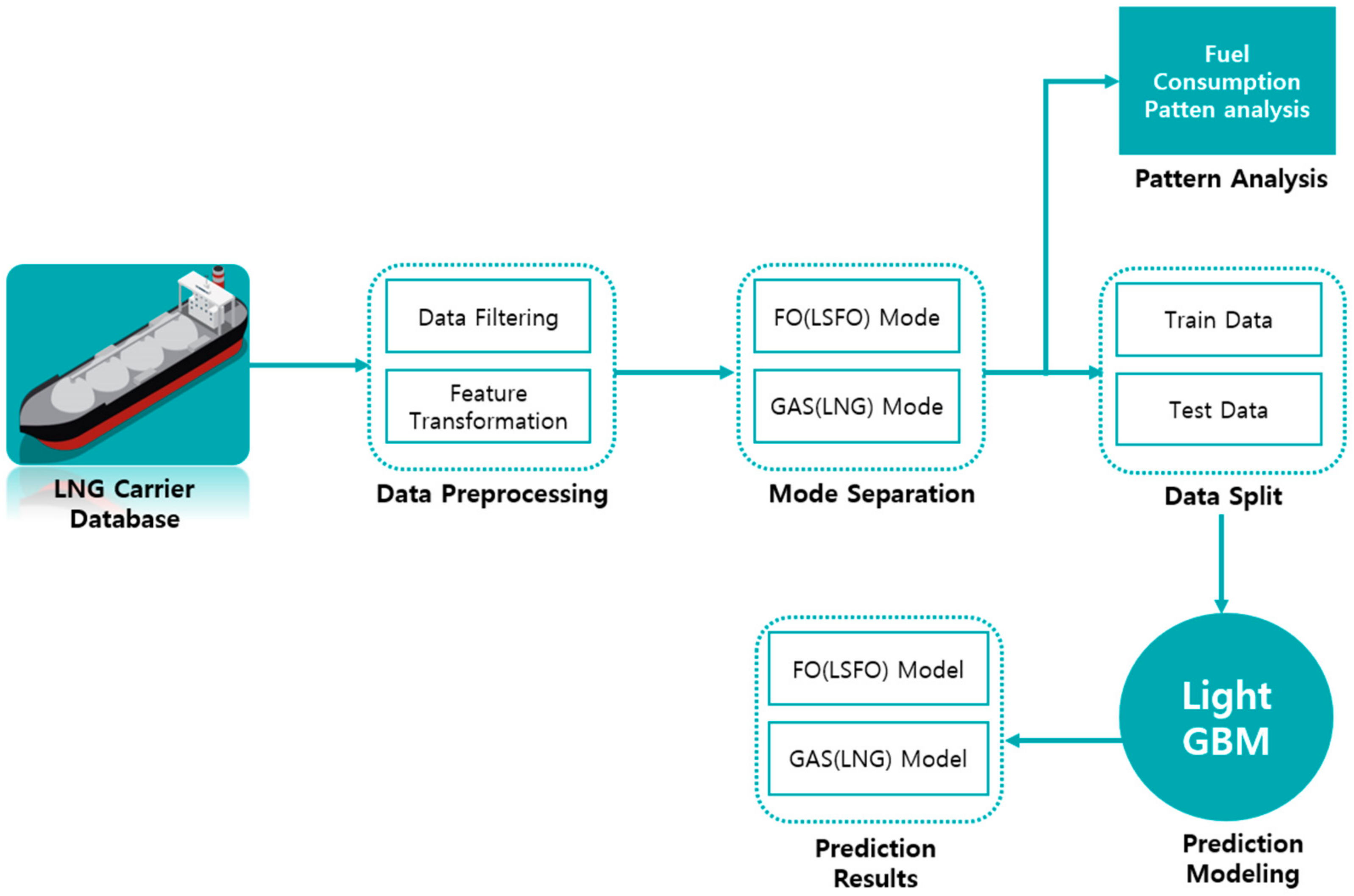
• Data Preprocessing: Missing values and outliers were removed, and medium- to high-speed segments, where fuel consumption is higher, were extracted.
• Mode Separation: Preprocessed data were separated by operation mode, distinguishing fuel oil (LSFO) sections from gas (LNG) sections.
• Fuel Consumption Pattern Analysis: Energy usage patterns and characteristics were analyzed for each voyage based on the separated modes.
• Data Split: The dataset was divided into training (80%) and testing (20%) sets to validate model performance.
• Prediction Modeling: LightGBM models were developed to predict fuel consumption for each mode.
• Prediction Results: Model accuracy was evaluated using RMSE, MAE, and R-squared (R²) on the test data.

4.1. Data Preprocessing

4.1.1. Data Filtering

The data collected from the target ship are primarily obtained from sensors attached to various ship equipment, which may result in missing values due to various factors. These factors include technical issues or physical damage to the sensors, communication errors, interruptions during data transmission, storage device problems, and environmental conditions.

When sensor anomalies occur, the data collection device records a value of −9999. Therefore, if the minimum value of a feature is −9999, it indicates the presence of missing data for that feature. To ensure data quality, instances with any missing values in any column were removed from the dataset.

In this study, the goal is to analyze fuel usage patterns through exploratory data analysis (EDA). Following this, the objective is to develop a fuel consumption prediction model for steady cruising conditions with ground speed recorded as 10 knots or higher. Therefore, only data where the ground speed was recorded as 10 knots or higher were used for model development. There are two primary reasons for this decision. First, most fuel consumption occurs during steady cruising conditions, making low-speed segment data less impactful. Second, low-speed segments often involve anchoring and course changes, which do not reflect typical sailing patterns and could reduce predictive accuracy.

4.1.2. Feature Transformation and Mode Separation

The target ship in this study is equipped with two main engines. Observations showed that the outputs related to each engine were largely consistent. To simplify the analysis, data from both engines were averaged for each feature, providing a unified view of engine performance. Similarly, draft measurements at the bow and stern were combined by averaging, creating a single draft indicator. This feature transformation process enables a deeper exploration of the ship’s operational patterns.

One of the objectives of this study is to understand the operational behavior and fuel usage patterns of dual-fuel ships, particularly how the ship transitions between fuel types and manages energy sources. The ship in this study exclusively uses Low Sulfur Fuel Oil (LSFO) as its fuel oil and LNG as its gas fuel. Consequently, the analysis defines four main fuel usage modes: FO mode (using fuel oil), GAS mode (using LNG), mixed mode (using both fuels simultaneously), and non-fuel mode when neither fuel is used.

To track fuel usage, three main indicators were established: FO usage, GAS usage, and combined usage. These indicators allow for the clear differentiation of the ship’s operational state and enable the analysis of fuel-switching behavior over time. Using these features, we analyzed the frequency and conditions under which the ship switches between fuel types, providing valuable insights into the fuel management strategies that can optimize efficiency and reduce environmental impact. This transformed feature set supports a comprehensive understanding of the dual-fuel system’s operations, as shown in

Table 3. Feature transformation lists.

Feature Name	Unit	Description
Main Engine Load	%	Average load of Main Engines 1 and 2
Main Engine Power	kW	Average output of Main Engines 1 and 2
Main Engine RPM	revolution/min	Average RPM of Main Engines 1 and 2
Main Engine FOC	kg/h	Average LSFO consumption of Main Engines 1 and 2
Main Engine GC	kg/h	Average LNG consumption of Main Engines 1 and 2
Draft	m	Average draught of Draught Fore and Draught Aft
FO_MODE	-	LSFO mode (Main Engine FOC ≥ 1)
GAS_MODE	-	LNG mode (Maine Engine GC ≥ 1)

.

4.2. Operational Pattern Analysis

The operational pattern analysis in this study was designed to investigate fuel consumption patterns in an LNG-fueled dual-fuel ship under various operational conditions. To achieve this, we first selected essential operational features related to fuel consumption, including speed over ground, Main Engine RPM, main engine load, main engine power output, Ship Heading, and draft. Data cleaning was conducted to ensure quality before proceeding with the analysis. Next, we applied time-series analysis to observe temporal changes in fuel mode usage across multiple voyages, which allowed us to identify trends and shifts in the fuel usage modes over time.

In the next phase, we created route maps to spatially segment each voyage by fuel mode. This mapping approach enabled us to identify specific sections along each route where fuel mode shifts occurred, providing a spatial perspective on fuel consumption behavior. To further understand fuel-switching behavior, we identified and analyzed instances of rapid transitions between the fuel oil (FO) and gas (GAS) modes, referred to as fuel changeover peaks. By correlating these peaks with operational factors such as speed changes, directional shifts, and engine load adjustments, we aimed to uncover the operational scenarios that commonly trigger fuel switching.

Finally, we performed a detailed classification of fuel usage patterns for each voyage, differentiating between steady cruising conditions and more dynamic navigational scenarios that required frequent fuel switching. Additionally, we examined how route complexity—such as straight versus winding sections—impacted fuel mode choices, especially in areas with frequent speed or course adjustments. This approach provided a comprehensive understanding of the factors driving fuel mode selection, contributing valuable insights toward developing optimized fuel management strategies for dual-fuel vessels.

4.3. Fuel Consumption Prediction Model

This study aims to classify the GAS and FO fuel modes, analyze operational pattern profiles, and develop predictive models tailored to each mode to optimize fuel management strategies. Using these models, we seek to accurately forecast fuel consumption patterns for each mode, enabling more efficient and effective fuel use [40].

In this study, the LightGBM model was selected as the prediction model. The dataset used is structured and time-series-based, making LightGBM the most suitable choice due to its superior performance with such data. Compared to other gradient boosting models, such as XGBoost and CatBoost, LightGBM has demonstrated superior performance in both prediction accuracy and computational efficiency, particularly for time-series data [41,42].

One of the key reasons for this choice is LightGBM’s leaf-wise tree growth strategy, which splits the leaf with the highest potential for loss reduction. This approach contrasts with the level-wise growth strategies used by XGBoost and CatBoost, allowing LightGBM to achieve higher accuracy and lower training loss, especially in datasets with complex relationships between variables. This efficiency is further enhanced by its histogram-based algorithm, which reduces memory usage and accelerates training without compromising accuracy [43]. Additionally, LightGBM employs Gradient-based One-Side Sampling (GOSS), a technique that selectively retains high-gradient instances while sampling low-gradient ones. This method not only reduces the data volume required for training but also ensures that critical information is preserved, a distinct advantage over XGBoost, which processes all data points equally, potentially leading to longer training times [44]. While CatBoost is optimized for categorical data and XGBoost offers strong baseline performance across diverse applications, LightGBM excels in processing datasets with continuous features and pronounced structural characteristics, such as time-series data. Its ability to capture nonlinear interactions and adapt to patterns within temporal data makes it particularly robust for this study. Moreover, LightGBM’s faster training speeds and lower computational demands make it a practical choice for large-scale datasets, aligning well with the study’s focus on predictive modeling [45,46]

Following model selection, we fine-tuned the model’s hyperparameters to maximize predictive performance. Bayesian optimization was employed for hyperparameter tuning, as it efficiently searches the parameter space by balancing exploration and exploitation, outperforming traditional methods like grid and random search. Key hyperparameters, including lambda_l1, lambda_l2, num_leaves, feature_fraction, bagging_fraction, and min_child_samples, were optimized to minimize Root Mean Squared Error (RMSE). The tuning process utilized 5-fold cross-validation on the training set to ensure that the model generalizes well to unseen data and captures complex patterns in fuel consumption without overfitting [47].

This comprehensive approach to model development and tuning enhances the model’s ability to predict fuel consumption accurately for each fuel mode, supporting optimized fuel management strategies and contributing to improved operational efficiency for dual-fuel vessels.

5. Result and Discussion

5.1. Operational Pattern Analysis

We conducted a comprehensive analysis of the operational profiles for each voyage of the target ship to gain a detailed understanding of its fuel management patterns. This analysis emphasizes the identification of fuel usage trends and the development of optimized predictive models tailored to the specific characteristics of each fuel type. The overarching objective is to enhance fuel management efficiency and to formulate a model that optimizes fuel utilization across various operational scenarios.

To facilitate this analysis, we examined the time-series graphs of the features most relevant to the ship’s fuel consumption. In these graphs, the blue line represents FO (fuel oil, kg/h), while the orange line represents GAS (gas, kg/h). The features shown, starting from the first graph, include the fuel usage mode (kg/h), speed over ground (SPEED_VG, knots), main engine revolutions per minute (ME_RPM, RPM), main engine load (ME_LOAD, %), main engine power output (ME_POWER, kW), the ship’s heading (SHIP HEADING, degrees), and draft (DRAFT, meters). The x-axis in all the graphs represents the time stamp (time in 10 min intervals).

In addition to the time-series graphs, the route maps utilize specific colors to denote the different fuel modes. In these maps, green indicates the FO mode, orange represents the GAS mode, red signifies the mixed mode, and gray shows the sections where no fuel was used.

5.1.1. Voyage 1: Speed-Induced Fuel Changeover Peaks

The analysis of fuel usage patterns for Voyage 1 revealed three distinct fuel changeover peaks. These peaks were all closely associated with changes in speed and direction, occurring when the ship transitioned from FO to GAS during its operation. The first and second peaks were observed at times when the ship’s speed over ground increased sharply. As shown in Figure 3, these two peaks occurred during the process of accelerating the ship, during which the engine load (ME Load) and output (ME Power) increased, resulting in a temporary rise in FO consumption. This indicates that the ship switched to the FO mode to obtain the necessary power during periods of increased propulsion demand. The third peak occurred when the ship’s heading changed abruptly. At this point, both the engine load and output increased, leading to a temporary surge in FO consumption. This suggests that the ship switched to the FO mode to secure the additional power needed for the directional change. Additionally, changes in the draft were observed during this process, indicating that the physical state changes associated with the directional shift may have influenced fuel consumption.

As shown in Figure 4, the analysis of the Voyage 1 route reveals a tendency for fuel mode switching to occur at points where the route changes abruptly. The enlarged section in the map highlights the areas where these mode switches were most concentrated. In Figure 4, orange indicates the GAS mode, green represents the FO mode, red shows the mixed mode, and gray indicates the sections where no fuel was used. Notably, at the points where the route changes, both the speed and direction shifted rapidly, making steady cruising difficult, leading to a switch to the FO mode.

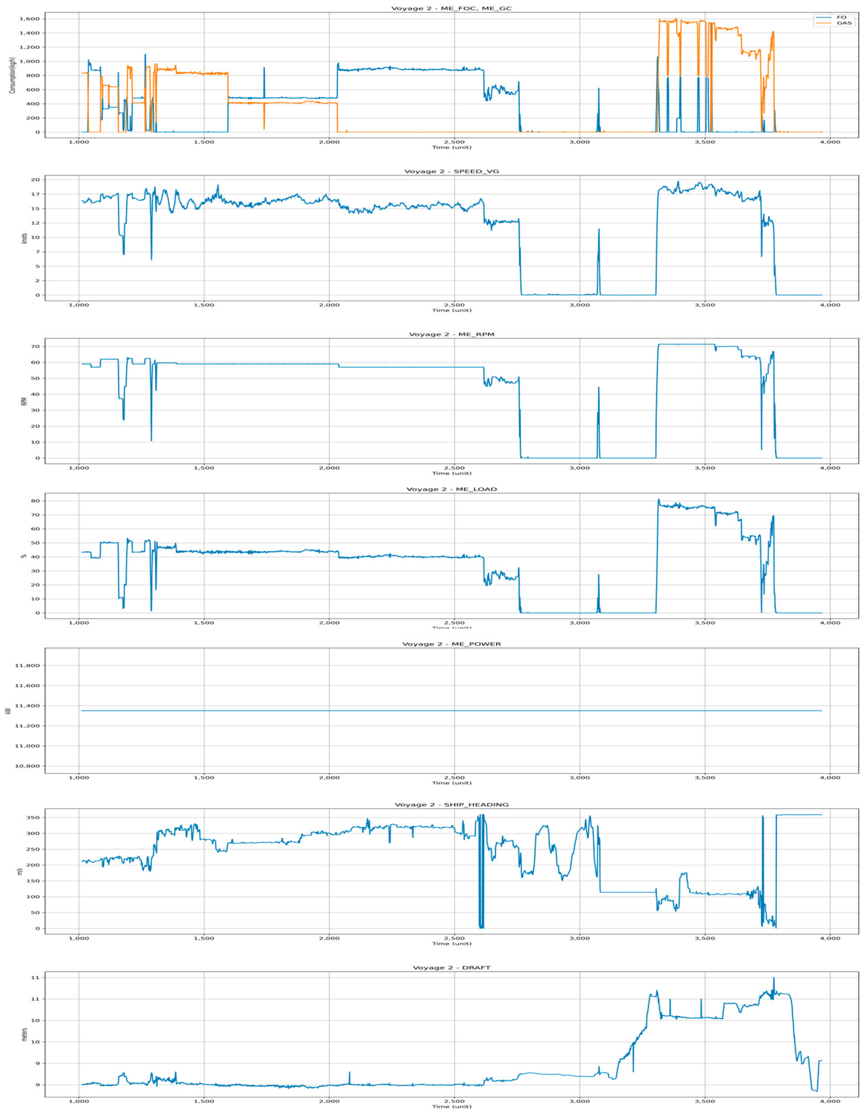
5.1.2. Voyage 2: Mixed Fuel Utilization and Directional Complexity

In Voyage 2, there were numerous instances where both FO and GAS were used in a mixed mode. As shown in Figure 4, fuel switching and mixed mode usage tended to occur primarily in conjunction with changes in speed over ground and Ship Heading. In the final gas usage section illustrated in Figure 5, the pattern shows that the ship switched to the FO mode when adjustments in draft or direction were necessary. This suggests that while gas fuel was employed for steady cruising, FO was likely used to complement the operation during speed changes or directional adjustments. Therefore, it can be inferred that the GAS mode is better suited for stable operations, whereas the FO mode is more appropriate for handling rapid changes in the ship’s operation.

In particular, as shown in Figure 6, the operational route of Voyage 2 indicates that the regions where the mixed mode was used align with specific points on the map, often occurring during course changes or in complex navigational areas. This suggests that the use of the mixed mode may arise from the ship’s intricate operational conditions.

The difficulty in clearly determining the exact reason for the use of the mixed mode may stem from the interplay of various operational variables. As observed in Figure 5, the areas where the mixed mode and FO mode were used are associated with specific routes, but this likely involves factors beyond simple speed or course changes, such as external environmental conditions or the complexity of the route.

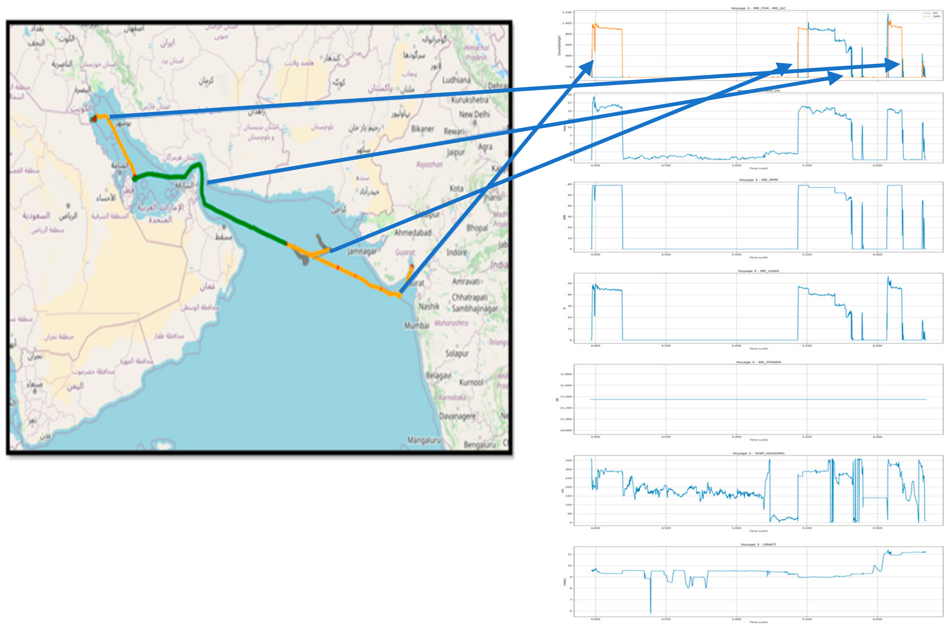
5.1.3. Voyage 3: Route Change Constraints on Fuel Switching

In Voyage 3, several fuel changeover peaks were observed during the ship’s operation (Figure 7). These peaks particularly occurred when the ship’s speed increased, before entering a stable speed zone, or when adjusting the course. During these moments, the ship operated in the FO mode, and once the operational conditions stabilized, it switched to the GAS mode. This phenomenon suggests that the ship tends to prefer FO fuel under unstable operational conditions, such as during speed changes or course adjustments. However, once the conditions stabilize, the ship switches to GAS to enhance fuel efficiency.

In Voyage 3, there were instances where the ship operated solely in the FO mode within specific sections (Figure 8). These sections primarily occurred in areas where frequent course changes took place, indicating that it might be challenging to use the GAS mode during situations with frequent route adjustments or course changes. Consequently, FO was exclusively used in these areas, demonstrating that course alterations are a significant factor that can restrict the use of the GAS mode. The areas include the Strait of Hormuz, the Gulf of Oman, and the coastal waters near Gujarat, India.

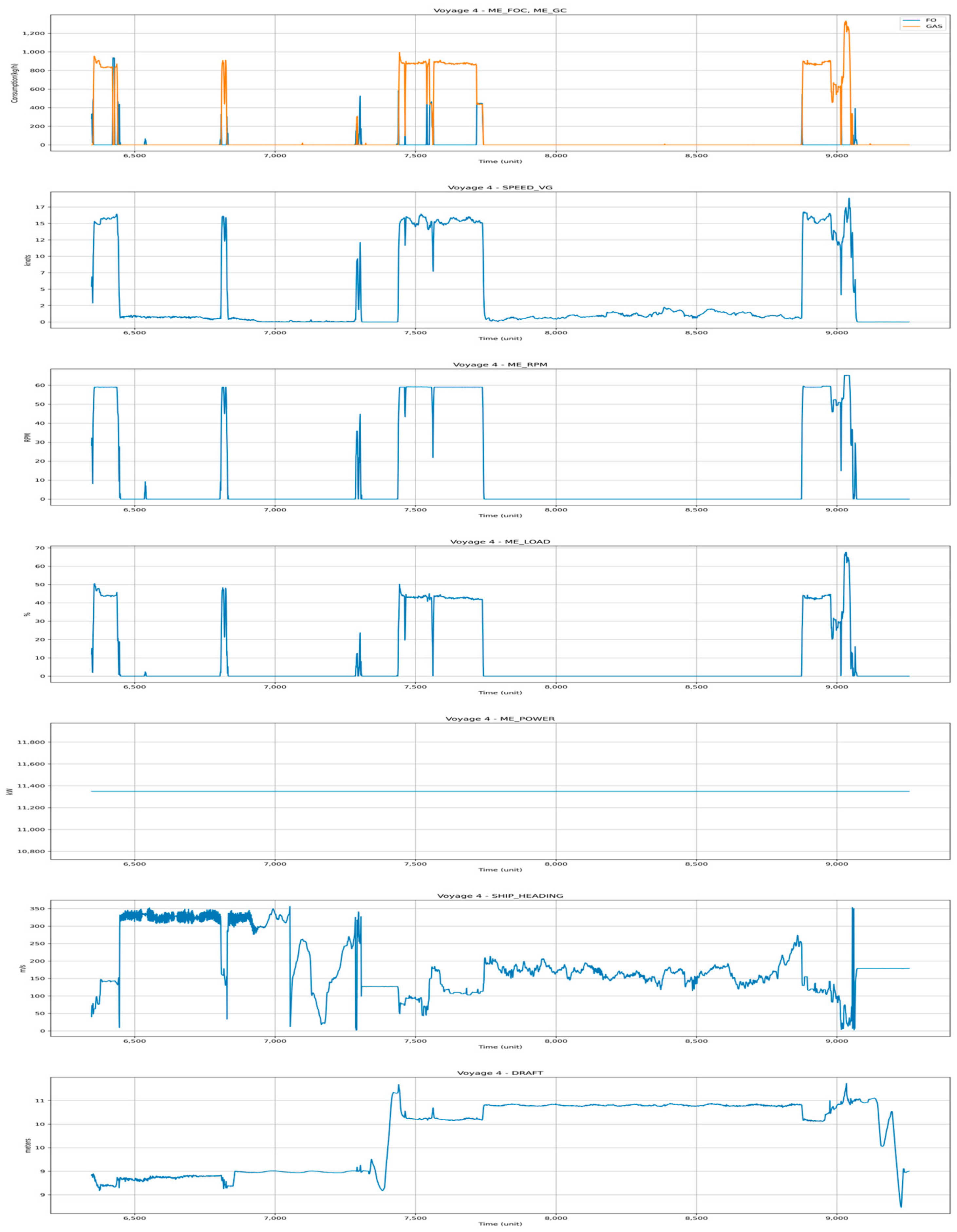
5.1.4. Voyage 4: Frequent Course Adjustments Leading to FO Spikes

The fuel consumption pattern in Voyage 4 shares several similarities with that of Voyage 1, but it also presents some key differences. Like in Voyage 1, three distinct fuel changeover peaks were observed in Voyage 4 (Figure 9). These peaks are closely associated with changes in speed over ground and Ship Heading. Similarly to Voyage 1, where the first and second peaks occurred when the ship was rapidly increasing speed and the third peak during a course change, Voyage 4 also exhibited fuel switchovers under these conditions.

However, a distinguishing factor is that while fuel changeovers in Voyage 1 primarily occurred during periods of speed increases and course changes, in Voyage 4, fuel switchovers were also observed during speed reductions. This suggests that Voyage 4 employed a more varied fuel transition strategy under different operational conditions compared to Voyage 1. The switch to the FO mode during speed reduction is a notable difference, indicating that fuel management strategies may vary between voyages, adapting to the specific conditions encountered. Additionally, as shown in Figure 10, the voyage route of Voyage 4 stands out due to the frequent course changes in complex sections. In these complex navigational areas, speed adjustments and course changes occurred frequently, leading to more frequent transitions to the FO mode. This suggests that the route of Voyage 4 involved more course alterations and complex operational conditions, indicating that the ship applied various fuel-switching strategies to navigate these sections safely and efficiently.

5.1.5. Voyage 5: Speed and Directional Variability Triggering Fuel Peaks

Several fuel changeover peaks were observed during Voyage 5, primarily occurring during moments of speed adjustment and course changes.

Three fuel changeover peaks, highlighted in red in Figure 11, were identified. These peaks were confirmed to coincide with significant fluctuations in the ship’s speed over ground and Ship Heading. The first peak occurred when the ship’s speed increased sharply, during which FO was utilized. Afterward, the ship transitioned to the GAS mode, maintaining a stable speed. The second peak occurred during a phase where both speed and directional adjustments were necessary. FO was predominantly used during this period, and once speed and direction stabilized, the ship switched back to the GAS mode. The third peak occurred immediately following another speed change, indicating that the ship initially used FO for high-speed operation before transitioning back to the GAS mode.

As shown in Figure 12, the operational route of Voyage 5 visually confirms the alignment between major route changes and the fuel changeover peaks. This analysis illustrates how fuel usage strategies shift under complex navigational conditions. The areas highlighted in orange and red particularly indicate the sections where FO was used. In contrast, the GAS mode was primarily utilized in the sections where the route remained straight, with minimal speed changes or directional adjustments.

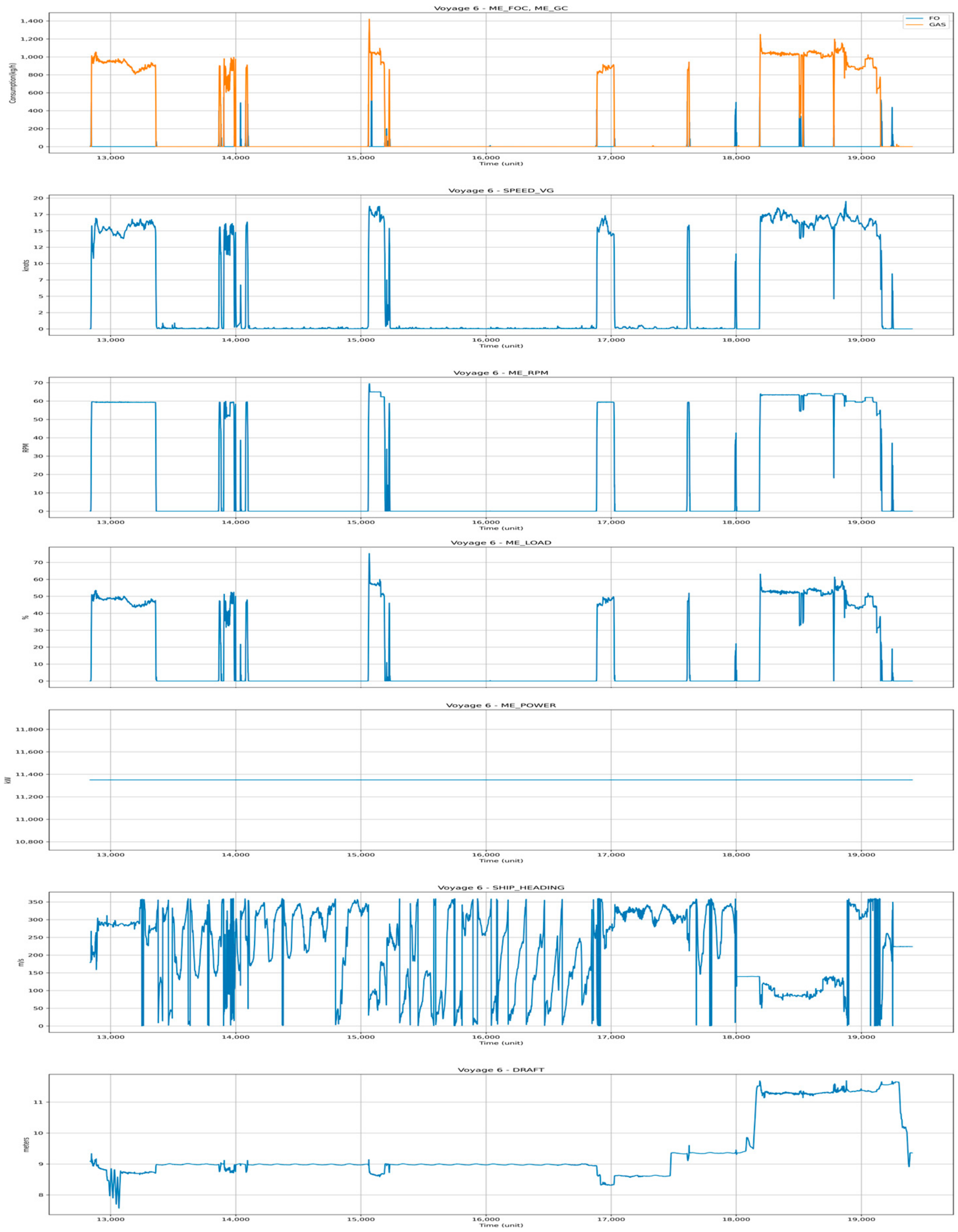
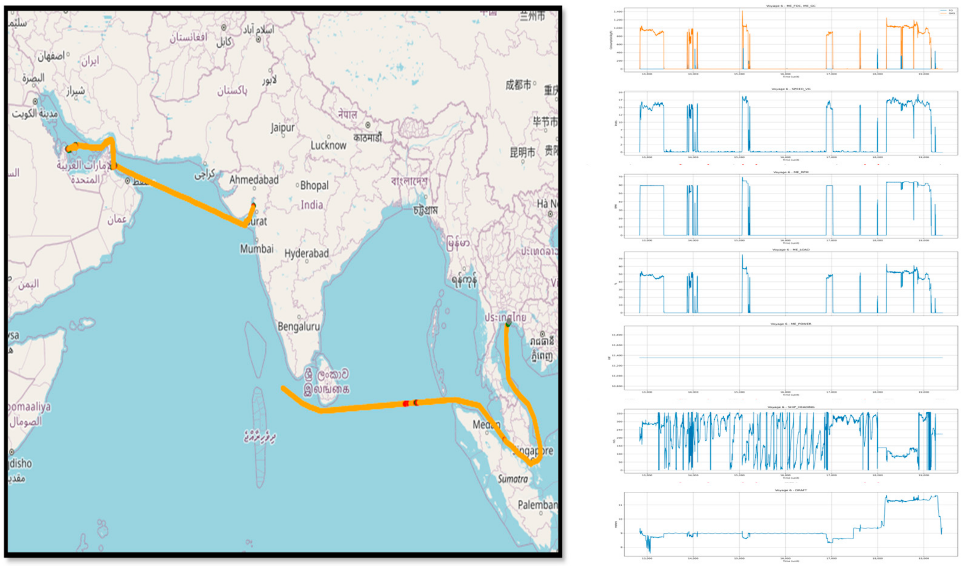
5.1.6. Voyage 6: Complex Navigation with Frequent Fuel Shifts

In Voyage 6, several fuel changeover peaks were observed, primarily occurring at times when changes in the ship’s speed and direction were necessary. As shown in Figure 13, three fuel changeover peaks marked in red can be identified. The first peak occurred when the ship’s speed over ground changed rapidly, prompting a switch to the FO mode. After this peak, the ship transitioned back to the GAS mode, which was then used consistently in the stabilized speed zones. The second peak occurred at a point where a directional change was made, accompanied by an increase in speed, leading to the use of FO. In this case, as well, once the direction and speed stabilized, the ship switched back to the GAS mode. The third peak took place when speed and direction adjustments were needed, after which the ship reverted to the GAS mode, leading to a stabilization of the operation.

As shown in Figure 14, the sections marked in orange and red are primarily located in complex navigational areas, where significant changes in the ship’s speed and direction occurred, leading to the use of FO. In contrast, the GAS mode was primarily used in the areas where a consistent speed and direction were maintained.

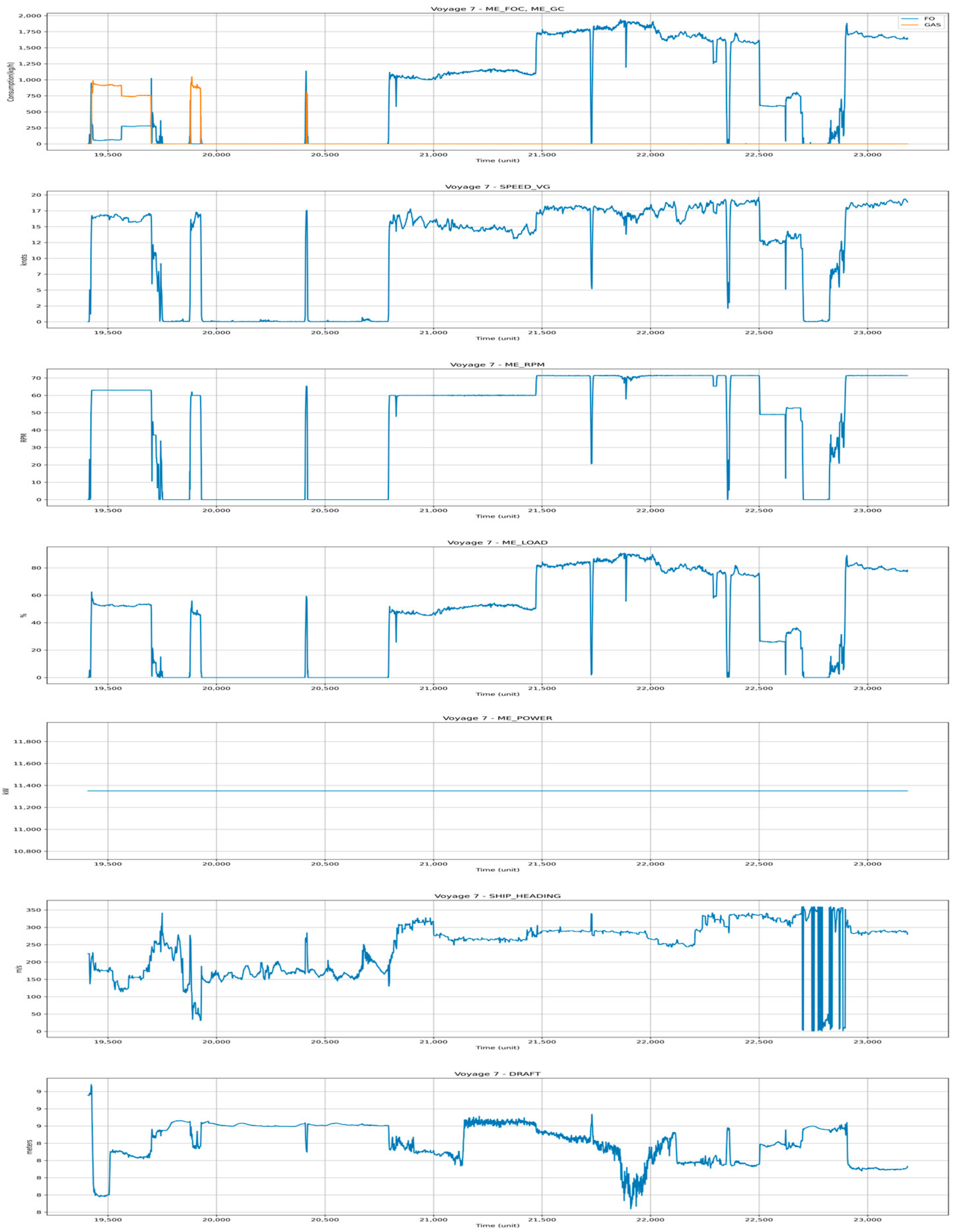
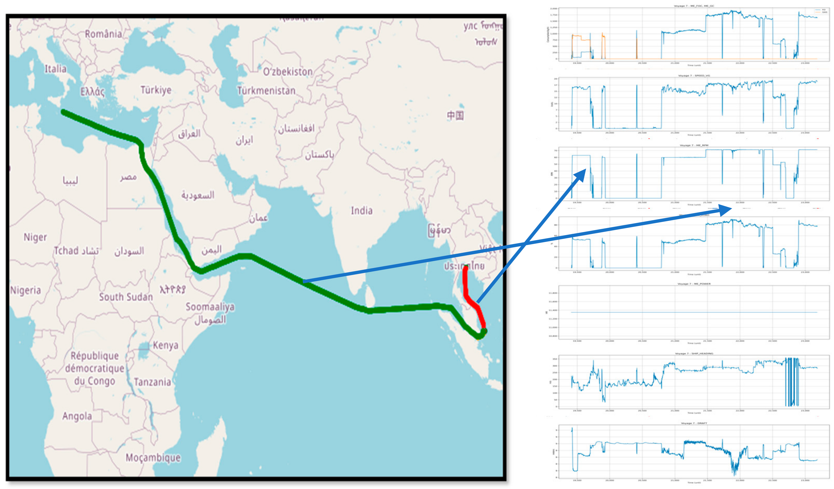
5.1.7. Voyage 7: Stable Navigation with Controlled Fuel Switches

In Voyage 7, several fuel changeover peaks were observed, with a particular emphasis on the relationship between speed changes and the use of FO. As shown in Figure 15, the graph indicates instances where fuel changeover peaks occurred alongside changes in the ship’s speed over ground. The first peak occurred when the speed fluctuated suddenly, prompting a switch to the FO mode, followed by a return to the GAS mode. This pattern suggests that FO was utilized during the segments where speed adjustments or course corrections were necessary. Additionally, in the later stages of the voyage, fuel usage stabilized, with the GAS mode being consistently maintained. This indicates that the ship efficiently used GAS fuel while maintaining stable speed and direction.

As shown in Figure 16, the sections where fuel changeover peaks occurred are visually identifiable. The route maintained a relatively consistent direction but also traversed some complex areas where speed adjustments were required. Consequently, the FO mode was engaged in these challenging sections to provide the necessary power, while the GAS mode was resumed in more stable segments.

As shown in Figure 16, the sections where fuel changeover peaks occurred are visually identifiable. The route maintained a relatively consistent direction but also traversed some complex areas where speed adjustments were required. Consequently, the FO mode was engaged in these challenging sections to provide the necessary power, while the GAS mode was resumed in more stable segments.

5.2. Prediction Model for Dual-Fuel Consumption

Hyperparameter tuning for the LightGBM model was performed using the Optuna library to optimize its performance. Optuna, based on an efficient Bayesian optimization algorithm, automatically searches for hyperparameter combinations and quickly finds high-performing hyperparameters to maximize the model’s predictive performance. During the tuning process, K-fold cross-validation was used to assess how well the model generalizes across different datasets. Specifically, Optuna first proposed hyperparameter combinations in each trial, and then 5-fold cross-validation was conducted. For each fold, the LightGBM model was trained with the proposed hyperparameter values, and the combination that minimized the RMSE (Root Mean Squared Error) on the validation dataset was selected (

Table 4. Hyperparameter tuning range and value.

Hyperparameter	Range	Best Value
lambda_l1	{0.0000001~10.0}	0.000305
lambda_l2	{0.0000001~10.0}	0.05957
num_leaves	{2~256}	207
feature_fraction	{0.4~1.0}	0.554
bagging_fraction	{1~7}	2
min_child_samples	{5~100}	5

).

The model was trained using the training dataset for both the GAS and FO modes, and the final accuracy was measured using 20% of the data reserved for testing. As shown in

Table 5. Performance metrics.

	R2 Score		RMSE		MAE
Mode	GAS	FO	GAS	FO	GAS	FO
Test	0.94	0.98	33.01	48.36	16.29	22.92

, the R² scores for GAS and FO were 0.94 and 0.98, respectively, indicating that both models closely follow the variance in actual fuel consumption. Moreover, in terms of RMSE and MAE, metrics that indicate the absolute accuracy of the predictions, the predictions for the GAS mode slightly outperformed those for the FO mode. For both models, the errors were below 50, which is significantly smaller compared to the standard deviations of FO consumption (677) and GAS consumption (456), indicating that the errors occurred within a relatively small range.

5.3. Discussion

The usage patterns of the FO mode and GAS mode during ship operations were analyzed, and fuel-switching strategies were explored in relation to complex routes and environmental factors. Additionally, fuel consumption prediction models were developed for each fuel mode, allowing an analysis of how ships can efficiently consume fuel under various operating conditions.

• FO Mode Usage Strategy: The analysis revealed that during most voyages, fuel changeover peaks were observed when the ship experienced abrupt changes in speed. FO was predominantly used when the ship needed to accelerate or make sharp directional changes. This indicates a preference for FO in situations requiring immediate power output, as it provides quicker propulsion compared to GAS. This pattern was particularly evident in Voyages 1, 3, 4, 5, and 6. Notably, in Voyage 4, the FO mode was engaged not only during periods of speed increase but also during speed reductions, highlighting a unique pattern observed in this voyage. For instance, in Voyage 1, FO was used to handle speed variations and heading changes, while in Voyage 4 and 5, it was necessary for sharp course adjustments in narrow waterways. Additionally, FO was utilized in congested straits during Voyage 6 to navigate external challenges such as vessel traffic and unpredictable weather (

  Table 6. Profile characteristics and fuel mode scenarios.

  Voy	Profile Characteristics	Fuel Mode	Scenario
  1	Open waters with speed variations	FO	FO was used to handle speed increases and decreases effectively, ensuring quick responsiveness during transitions.
  	Directional adjustments at key points	FO	Necessary to provide sufficient power during heading changes, ensuring stable maneuverability.
  	Stable cruising	GAS	GAS was used for sustained cruising with minimal fluctuations, reducing emissions and fuel costs.
  2	Complex route with frequent adjustments	Mixed	Mixed mode was used for narrow waterways and sharp course changes, balancing FO’s power and GAS’s efficiency.
  	Stable cruising segments	GAS	Preferred for long, straight sections where minimal adjustments are required.
  	Sharp directional changes	FO	Required for maintaining stability and responsiveness during abrupt course adjustments.
  3	Frequent course changes	FO	Used to handle unstable conditions with frequent adjustments in heading and speed.
  	Speed variations in open waters	FO	Critical for acceleration and deceleration phases in variable-speed regions.
  	Prolonged steady-state operations	GAS	Utilized in stable, open-water sections with consistent speeds to maximize efficiency.
  4	Narrow waterways, frequent course adjustments	FO	Required during rapid speed changes and sharp course adjustments to maintain maneuverability.
  	Calm, straight sections	GAS	Used during steady cruising for optimal fuel efficiency.
  5	Tight navigational paths	FO	Critical for overcoming environmental resistance and navigating through complex, winding paths.
  	Open water between narrow sections	GAS	Enables sustained cruising at consistent speeds between confined navigational areas.
  6	Congested or busy straits	FO	Necessary to handle external challenges, including nearby vessel traffic and unpredictable weather.
  	Clear straits or open stretches	GAS	Preferred for low-demand routes with reduced complexity.
  7	Prolonged narrow passages	Mixed	Combines FO’s high-power availability with GAS’s cost efficiency for intricate navigational situations.
  	Minimal adjustment regions	GAS	Focused on maintaining emissions compliance and minimizing operational costs during stable navigation.

  ). These findings suggest that FO offers better maneuverability and responsiveness under unstable route conditions.
• Gas Mode Usage Strategy: The GAS mode was primarily used in stable operating conditions where the ship could maintain consistent speed and direction. This reflects a strategy aimed at maximizing fuel efficiency, given that GAS is more economical, making it preferable during steady-state operations. This pattern was observed in Voyages 1, 3, 4, 5, and 7. For example, in Voyages 1 and 7, GAS was consistently maintained during prolonged cruising in open waters, ensuring reduced emissions and fuel costs. Similarly, in Voyage 5, GAS was predominantly used on relatively straight routes, while in Voyage 6, it was preferred for open stretches with low navigational demand (Table 6). These findings highlight the GAS mode’s suitability for stable and efficient operations.
• Flexibility of Mixed Fuel Mode: As observed in Voyage 2, the ship occasionally employed a mixed mode of FO and GAS to adapt to complex route conditions or external environmental changes. This strategy appears to aim at maintaining safe and efficient navigation by flexibly switching fuel modes to accommodate various operational conditions. For example, in Voyage 2, the mixed mode was used during narrow waterways and sharp course changes to balance FO’s power and GAS’s efficiency. Similarly, in Voyage 7, the mixed mode was employed in prolonged narrow passages, effectively combining the advantages of both fuels for intricate navigational scenarios (Table 6).
• In summary, the FO mode was ideal for dynamic and unstable conditions requiring immediate power, the GAS mode was suited for stable cruising, and the mixed mode provided versatility in complex operational situations. These findings underline the importance of tailored fuel-switching strategies to optimize both operational performance and environmental outcomes.

6. Conclusions

This study focused on analyzing the operational data of dual-fuel ships that use GAS and FO modes, exploring fuel-switching patterns based on complex routes and environmental factors, and developing fuel consumption prediction models tailored to each fuel mode. The FO mode was primarily used in situations requiring sudden speed changes or directional shifts, while the GAS mode was mainly employed on stable routes to maximize fuel efficiency. Through this operational pattern analysis, we were able to identify the key moments and conditions under which fuel switching occurs.

Additionally, this study considered key variables such as weather conditions, cargo load, and engine performance, fully reflecting the various factors that affect fuel consumption. This allowed for the development of a more precise and reliable fuel consumption prediction model which can serve as a foundational resource for future carbon emission measurements and fuel management strategy development.

The prediction model developed using LightGBM achieved R² scores of 0.94 for the GAS mode and 0.98 for the FO mode, demonstrating high prediction accuracy. This enabled the precise prediction of fuel consumption patterns for each fuel mode under various operational conditions.

However, since this study was conducted based on data from a specific ship, further validation is required to generalize the findings to various ship types and operating environments. Therefore, future research should utilize more diverse ship datasets to broaden the applicability of the results. Additionally, it appears that decisions by navigators or ship operators partially influence the selection and switching of fuel modes, making it challenging to precisely predict the timing of fuel mode transitions solely with machine learning models.

Nevertheless, this study provides essential foundational data for ensuring compliance with carbon emission regulations and improving fuel efficiency in the maritime industry. The model, which accurately predicts fuel consumption, offers ship operators practical fuel management strategies that contribute not only to reducing fuel costs but also to developing policies and operational strategies aimed at achieving carbon neutrality. In particular, this model serves as valuable reference material for the development of carbon reduction strategies to meet the increasingly stringent environmental regulations set by IMO.

Furthermore, this study offers insights that are applicable not only to the maritime industry but also to the global logistics and shipping sectors. By establishing effective fuel management and operational strategies for ships, it provides practical support in maximizing energy efficiency and minimizing environmental impact.

References

1. Huang, M.T.; Zhai, P.M. Achieving Paris Agreement Temperature Goals Requires Carbon Neutrality by Middle Century with Far-Reaching Transitions in the Whole Society. Adv. Clim. Change Res. 2021, 12, 281–286. [Google Scholar] [CrossRef]
2. Schreyer, F.; Luderer, G.; Rodrigues, R.; Pietzcker, R.C.; Baumstark, L.; Sugiyama, M.; Brecha, R.J.; Ueckerdt, F. Common but Differentiated Leadership: Strategies and Challenges for Carbon Neutrality by 2050 across Industrialized Economies. Environ. Res. Lett. 2020, 15, 114016. Available online: https://iopscience.iop.org/article/10.1088/1748-9326/abb852 (accessed on 16 October 2020). [CrossRef]
3. Timofeev, G.; Podkolzin, P.; Gladilin, D. Global Trends and Challenges of Achieving Carbon Neutrality. Russ. J. Resour. Conserv. Recycl. 2022, 9, 1–14. [Google Scholar] [CrossRef]
4. IMO. Second IMO Greenhouse Gas Study 2009; International Maritime Organization (IMO): London, UK, 2009; Available online: https://wwwcdn.imo.org/localresources/en/OurWork/Environment/Documents/SecondIMOGHGStudy2009.pdf (accessed on 1 April 2009).
5. IMO. Fourth IMO Greenhouse Gas Study 2020: Executive Summary; International Maritime Organization (IMO): London, UK, 2020; Available online: https://wwwcdn.imo.org/localresources/en/OurWork/Environment/Documents/Fourth IMO GHG Study 2020 Executive-Summary.pdf (accessed on 4 August 2020).
6. Maritime, I.; Traffic, T. International Maritime Trade and Port Traffic; United Nations: New York, NY, USA, 2021; pp. 1–33. [Google Scholar] [CrossRef]
7. UNCTAD. Review of Maritime Transport 2020: International Maritime Trade and Port Traffic; United Nations Conference on Trade and Development (UNCTAD): New York, NY, USA, 2021; Available online: https://unctad.org/system/files/official-document/rmt2020_en.pdf (accessed on 1 October 2024).
8. Rahim, M.M.; Islam, M.T.; Kuruppu, S. Regulating Global Shipping Corporations’ Accountability for Reducing Greenhouse Gas Emissions in the Seas. Mar. Policy 2016, 69, 159–170. [Google Scholar] [CrossRef]
9. López-Aparicio, S.; Tønnesen, D.; Thanh, T.N.; Neilson, H. Shipping Emissions in a Nordic Port: Assessment of Mitigation Strategies. Transp. Res. Part D Transp. Environ. 2017, 53, 205–216. Available online: https://www.sciencedirect.com/science/article/abs/pii/S1361920915300481 (accessed on 26 April 2017). [CrossRef]
10. Bortuzzo, V.; Bertagna, S.; Bucci, V. Mitigation of CO2 Emissions from Commercial Ships: Evaluation of the Technology Readiness Level of Carbon Capture Systems. Energies 2023, 16, 3646. [Google Scholar] [CrossRef]
11. IMO. Resolution MEPC.304(72) (Adopted on 13 April 2018) Initial IMO Strategy on Reduction of GHG Emissions from Ships; International Maritime Organization (IMO): London, UK, 2018; Available online: https://wwwcdn.imo.org/localresources/en/KnowledgeCentre/IndexofIMOResolutions/MEPCDocuments/MEPC.304(72).pdf (accessed on 13 April 2018).
12. IMO. Resolution MEPC.377(80), Annex 15, 2023 IMO Strategy on Reduction of GHG Emissions from Ships; International Maritime Organization (IMO): London, UK, 2023; Available online: https://wwwcdn.imo.org/localresources/en/KnowledgeCentre/IndexofIMOResolutions/MEPCDocuments/MEPC.377(80).pdf (accessed on 7 July 2023).
13. IMO. IMO Train the Trainer (TTT) Course on Energy Efficient Ship Operation Module 2—Ship Energy Efficiency Regulations and Related Guidelines; International Maritime Organization (IMO): London, UK, 2016; Available online: https://wwwcdn.imo.org/localresources/en/OurWork/Environment/Documents/Air pollution/M2 EE regulations and guidelines final.pdf (accessed on 1 January 2016).
14. IMO. 2013 Guidelines for Calculation of Reference Lines for Use with the Energy Efficiency Design Index (EEDI), Resolution MEPC.231(65); International Maritime Organization (IMO): London, UK, 2013; Available online: https://wwwcdn.imo.org/localresources/en/KnowledgeCentre/IndexofIMOResolutions/MEPCDocuments/MEPC.231(65).pdf (accessed on 17 May 2013).
15. IMO. Amendments to the Annex of the Protocol of 1997 to Amend the International Convention for the Prevention of Pollution from Ships, 1973, as Modified by the Protocol of 1978 Relating Thereto (Revised MARPOL Annex VI), Resolution MEPC.328(76); International Maritime Organization (IMO): London, UK, 2021; Available online: https://wwwcdn.imo.org/localresources/en/KnowledgeCentre/IndexofIMOResolutions/MEPCDocuments/MEPC.328(76).pdf (accessed on 17 June 2021).
16. ABS. Guide for Smart Functions for Marine Vessels and Offshore Units; American Bureau of Shipping (ABS): Texas, TX, USA, 2022; Available online: https://ww2.eagle.org/content/dam/eagle/rules-and-guides/current/other/307_smart_functions_marine_offshore_2022/smart-guide-jun22.pdf (accessed on 1 June 2022).
17. Rachow, M.; Loest, S.; Sitinjak, L.R.M. Concept for a LNG Gas Handling System for a Dual Fuel Engine. Int. J. Mar. Eng. Innov. Res. 2017, 1, 272–283. [Google Scholar] [CrossRef]
18. Livaniou, S.; Chatzistelios, G.; Lyridis, D.V.; Bellos, E. LNG vs. MDO in Marine Fuel Emissions Tracking. Sustainability 2022, 14, 3860. [Google Scholar] [CrossRef]
19. Iannaccone, T.; Landucci, G.; Tugnoli, A.; Salzano, E.; Cozzani, V. Sustainability of Cruise Ship Fuel Systems: Comparison among LNG and Diesel Technologies. J. Clean. Prod. 2020, 260, 121069. [Google Scholar] [CrossRef]
20. Xing, H.; Stuart, C.; Spence, S.; Chen, H. Alternative Fuel Options for Low Carbon Maritime Transportation: Pathways to 2050. J. Clean. Prod. 2021, 297, 126651. [Google Scholar] [CrossRef]
21. Ng, C.K.L.; Liu, M.; Lam, J.S.L.; Yang, M. Accidental release of ammonia during ammonia bunkering: Dispersion behaviour under the influence of operational and weather conditions in Singapore. J. Hazard. Mater. 2023, 452, 131281. [Google Scholar] [CrossRef] [PubMed]
22. McKinlay, C.J.; Turnock, S.R.; Hudson, D.A. Route to Zero Emission Shipping: Hydrogen, Ammonia or Methanol? Int. J. Hydrogen Energy 2021, 46, 28282–28297. [Google Scholar] [CrossRef]
23. Kim, Y.R.; Jung, M.; Park, J.B. Development of a Fuel Consumption Prediction Model Based on Machine Learning Using Ship In-Service Data. J. Mar. Sci. Eng. 2021, 9, 137. [Google Scholar] [CrossRef]
24. Hu, Z.; Jin, Y.; Hu, Q.; Sen, S.; Zhou, T.; Osman, M.T. Prediction of Fuel Consumption for Enroute Ship Based on Machine Learning. IEEE Access 2019, 7, 119497–119505. Available online: https://ieeexplore.ieee.org/document/8790676 (accessed on 1 October 2024). [CrossRef]
25. Ahlgren, F.; Mondejar, M.E.; Thern, M. Predicting Dynamic Fuel Oil Consumption on Ships with Automated Machine Learning. Energy Procedia 2019, 158, 6126–6131. [Google Scholar] [CrossRef]
26. Handayani, M.P.; Kim, H.; Lee, S.; Lee, J. Navigating Energy Efficiency: A Multifaceted Interpretability of Fuel Oil Consumption Prediction in Cargo Container Vessel Considering the Operational and Environmental Factors. J. Mar. Sci. Eng. 2023, 11, 2165. [Google Scholar] [CrossRef]
27. Li, S.; Li, X.; Zuo, Y.; Li, T. Prediction of Ship Fuel Consumption Based on Elastic Network Regression Model. In Proceedings of the 2021 International Conference on Information, Cybernetics, and Computational Social Systems, ICCSS 2021, Beijing, China, 10–12 December 2021; Institute of Electrical and Electronics Engineers Inc.: New York, NY, USA, 2021; pp. 296–301. Available online: https://ieeexplore.ieee.org/stamp/stamp.jsp?tp=&arnumber=9721951 (accessed on 10 December 2021).
28. Papandreou, C.; Ziakopoulos, A. Predicting VLCC Fuel Consumption with Machine Learning Using Operationally Available Sensor Data. Ocean. Eng. 2022, 243, 110321. [Google Scholar] [CrossRef]
29. Sui, C.; de Vos, P.; Stapersma, D.; Visser, K.; Ding, Y. Fuel Consumption and Emissions of Ocean-Going Cargo Ship with Hybrid Propulsion and Different Fuels over Voyage. J. Mar. Sci. Eng. 2020, 8, 588. [Google Scholar] [CrossRef]
30. Afon, Y.; Ervin, D. An Assessment of Air Emissions from Liquefied Natural Gas Ships Using Different Power Systems and Different Fuels. J. Air Waste Manag. Assoc. 2008, 58, 404–411. [Google Scholar] [CrossRef]
31. Pokhrel, S. Resolution MEPC.391(81) (Adopted on 22 March 20 24) 2024 Guidelines on Life Cycle GHG Intensity of Marine Fuels; International Maritime Organization (IMO): London, UK, 2024; pp. 37–48. Available online: https://wwwcdn.imo.org/localresources/en/KnowledgeCentre/IndexofIMOResolutions/MEPCDocuments/MEPC.391(81).pdf (accessed on 22 March 2024).
32. Bouabidi, Z.; Almomani, F.; Al-Musleh, E.I.; Katebah, M.A.; Hussein, M.M.; Shazed, A.R.; Karimi, I.A.; Alfadala, H. Study on Boil-off Gas (Bog) Minimization and Recovery Strategies from Actual Baseload Lng Export Terminal: Towards Sustainable Lng Chains. Energies 2021, 14, 3748. [Google Scholar] [CrossRef]
33. Shih, Y.C.; Tzeng, Y.A.; Cheng, C.W.; Huang, C.H. Speed and Fuel Ratio Optimization for a Dual-Fuel Ship to Minimize Its Carbon Emissions and Cost. J. Mar. Sci. Eng. 2023, 11, 758. [Google Scholar] [CrossRef]
34. Trodden, D.G.; Murphy, A.J.; Pazouki, K.; Sargeant, J. Fuel Usage Data Analysis for Efficient Shipping Operations. Ocean Eng. 2015, 110, 75–84. [Google Scholar] [CrossRef]
35. Lee, J.; Eom, J.; Park, J.; Jo, J.; Kim, S. The Development of a Machine Learning-Based Carbon Emission Prediction Method for a Multi-Fuel-Propelled Smart Ship by Using Onboard Measurement Data. Sustainability. 2024, 16, 2381. [Google Scholar] [CrossRef]
36. Li, S.; Zhang, P.; Sun, Z. Optimization of Fuel Supply Strategy for LNG Dual-Fuel Ships. J. Phys. Conf. Ser. 2022, 2491, 012014. Available online: https://iopscience.iop.org/article/10.1088/1742-6596/2491/1/012014/pdf (accessed on 16 December 2022). [CrossRef]
37. Martinić-Cezar, S.; Bratić, K.; Jurić, Z.; Račić, N. Exhaust Emissions Reduction and Fuel Consumption from the LNG Energy System Depending on the Ship Operating Modes. Pomorstvo 2022, 36, 338–349. [Google Scholar] [CrossRef]
38. Gelman, A. Exploratory Data Analysis for Complex Models. J. Comput. Graph. Stat. 2004, 13, 755–779. [Google Scholar] [CrossRef]
39. Morgenthaler, S. Exploratory Data Analysis. Wiley Interdiscip. Rev. Comput. Stat. 2009, 1, 33–44. [Google Scholar] [CrossRef]
40. Vorkapić, A.; Radonja, R.; Martinčić-Ipšić, S. Predicting Seagoing Ship Energy Efficiency from the Operational Data. Sensors 2021, 21, 2832. [Google Scholar] [CrossRef]
41. Németh, M.; Borkin, D.; Michalconok, G. The Comparison of Machine-Learning Methods XGBoost and LightGBM to Predict Energy Development. AISC 2019, 1047, 208–215. Available online: https://link.springer.com/chapter/10.1007/978-3-030-31362-3_21 (accessed on 20 September 2019).
42. Zhang, J.; Mucs, D.; Norinder, U.; Svensson, F. LightGBM: An Effective and Scalable Algorithm for Prediction of Chemical Toxicity-Application to the Tox21 and Mutagenicity Data Sets. J. Chem. Inf. Model. 2019, 44, 4150–4158. [Google Scholar] [CrossRef]
43. Min, F.; Yaling, L.; Xi, Z.; Huan, C.; Yaqian, H.; Libo, F.; Qing, Y. Fault Prediction for Distribution Network Based on CNN and LightGBM Algorithm. In Proceedings of the 2019 14th IEEE International Conference on Electronic Measurement & Instruments (ICEMI), Changsha, China, 1–3 November 2019; pp. 1020–1026. Available online: https://ieeexplore.ieee.org/document/9101423 (accessed on 1 October 2024).
44. Chen, X.; Zhang, H.; Bai, H.; Yang, C.; Zhao, X.; Li, B. Runtime Prediction of High-Performance Computing Jobs Based on Ensemble Learning. In Proceedings of the 2020 4th International Conference on High Performance Compilation, Computing and Communications, Association for Computing Machinery, Guangzhou, China, 27–29 June 2020; pp. 56–62. [Google Scholar] [CrossRef]
45. Hartanto, A.D.; Kholik, Y.N.; Pristyanto, Y. Stock Price Time Series Data Forecasting Using the Light Gradient Boosting Machine (LightGBM) Model. Int. J. Inf. Vis. 2023, 7, 2270–2279. [Google Scholar] [CrossRef]
46. Kumar, V.; Kedam, N.; Sharma, K.V.; Mehta, D.J.; Caloiero, T. Advanced Machine Learning Techniques to Improve Hydrological Prediction: A Comparative Analysis of Streamflow Prediction Models. Water 2023, 15, 2572. [Google Scholar] [CrossRef]
47. Wang, Y.; Wang, T. Application of Improved LightGBM Model in Blood Glucose Prediction. Appl. Sci. 2020, 10, 3227. [Google Scholar] [CrossRef]
Figure 1. Ship voyage trajectory (routes across Asia, India, the Middle East, and Europe).
Jmse 12 02235 g001
Figure 2. Research procedure.
Jmse 12 02235 g002
Figure 3. Voyage 1 operational analysis results.
Jmse 12 02235 g003
Figure 4. Voyage 1 route analysis results (near southern China’s coast, the central South China Sea, and Vietnam’s eastern coastal waters).
Jmse 12 02235 g004
Figure 5. Voyage 2 operational analysis results.
Jmse 12 02235 g005
Figure 6. Voyage 2 route analysis results (near the Strait of Hormuz, the Arabian Sea, the Bay of Bengal, and the Strait of Malacca).
Jmse 12 02235 g006
Figure 7. Voyage 3 operational analysis results.
Jmse 12 02235 g007
Figure 8. Voyage 3 route analysis results (the Strait of Hormuz, the Gulf of Oman, and the coastal waters near Gujarat, India).
Jmse 12 02235 g008
Figure 9. Voyage 4 operational analysis results.
Jmse 12 02235 g009
Figure 10. Voyage 4 route analysis results (the Strait of Hormuz, the Gulf of Oman, and the coastal waters near Gujarat, India).
Jmse 12 02235 g010
Figure 11. Voyage 5 operational analysis results.
Jmse 12 02235 g011
Figure 12. Voyage 5 route analysis results (near the Strait of Hormuz, the Gulf of Oman, and the coastal waters near Gujarat and Mumbai in India).
Jmse 12 02235 g012
Figure 13. Voyage 6 route analysis results.
Jmse 12 02235 g013
Figure 14. Voyage 6 route analysis results (near the Strait of Hormuz, the Gulf of Oman, the coastal waters near Gujarat and Mumbai, and the Strait of Malacca).
Jmse 12 02235 g014
Figure 15. Voyage 7 route analysis results.
Jmse 12 02235 g015
Figure 16. Voyage 7 route analysis results (the Bab-el-Mandeb Strait, the Gulf of Aden, and the southern coastal waters of India).
Jmse 12 02235 g016