Adaptive Sliding Mode Fault-Tolerant Tracking Control for Underactuated Unmanned Surface Vehicles

Abstract

This article proposes an adaptive sliding mode fault-tolerant tracking control scheme for underactuated unmanned surface vehicles (USVs) that suffer from loss of effectiveness and increase in bias input when performing path tracking. First, the mathematical model and fault model of USVs are introduced. Then, the USV is driven along the planned path by back-stepping and fast terminal sliding mode control. The radial basis function (RBF) neural network is used to approximate the unknown external disturbances caused by wind, waves, and currents, the unmodeled dynamics of the system, the actuator non-executed portions and bias faults. An adaptive law is designed to account for the loss of effectiveness of the thruster. In addition, through the analysis of Lyapunov stability criteria, it is proved that the proposed control method can asymptotically converge the tracking error to zero. Finally, this paper uses a simulation to demonstrate that, when a fault occurs, the tracking effect of the fault-tolerant control method proposed in this paper is almost the same as that without a fault, which proves the effectiveness of the designed adaptive law.

1. Introduction

In recent years, with the rapid development of control technology, USVs play an increasingly important role in marine activities such as marine resource exploration, marine search and rescue, and reconnaissance [1,2,3,4,5]. According to the actuator configuration, ships can be generally categorized into underactuated and fully actuated ships. Ships with higher requirements for control accuracy and safety, such as containers, drilling platforms, and special ships, are designed with full drive systems. In actual navigation, most ships, in order to economize, are only fitted with propellers to generate longitudinal propulsion and rudder devices to generate turning torque, not transverse propellers, which means they qualify as underdrive systems. Due to the complexity and variability of marine conditions, the propellers of fully driven ships frequently experience malfunctions or damages, at which time the system also becomes underactuated. The study of underactuated USV control is critical: underactuated USVs can be designed as backup controllers for fully driven USVs, which can reduce the catastrophic consequences brought about by the damage of the drive.

The basic tasks that underactuated ship motion control addresses today include point-to-point motion control, trajectory tracking control, path following control, dynamic positioning, and formation control, of which the path following problem of underactuated ships has received extensive attention in both theory and practical applications [6,7,8,9]. USVs are typical non-complete systems and have nonlinear characteristics and unknown perturbations in the marine environment, which makes the high-precision path tracking control of USVs extremely challenging. When the underactuated USV performs some tasks with high attitude requirements, the sideslip phenomenon caused by uncontrollable nonzero sway velocity is not allowed. Ref. [10] proposes a path following control algorithm for underactuated USVs, which can reduce the sideslip angle on a curved path. In [11], a fixed-time predictor is proposed to approximate the sideslip caused by disturbance for the path tracking problem of USV systems with unknown disturbance. The predictor can make the prediction error converge to zero in a fixed time. Ref. [12] proposes a finite-time integral line-of-sight-based path following a control scheme for four degree-of-freedom underactuated USVs in the presence of uncertain dynamics and environmental disturbances. It is worth noting that the states and inputs of USVs are either physically constrained or limited by marine applications. Ref. [13] investigates the trajectory tracking control problem of an underactuated unmanned vessel by means of a nonlinear model predictive control strategy under the presence of the above constraints of the system.

Because USVs work in uncertain and complex marine environments for a long time, coupled with factors such as aging components, they are prone to propulsion failures, and once a failure occurs, it is very likely to cause mission failure [14,15]. Therefore, fault-tolerant control technology has always been a problem of interest to USV researchers. Fault-tolerant control is categorized into active fault-tolerant control and passive fault-tolerant control. Active fault-tolerant control requires a fault detection module. For instance, ref. [16] presents a method for detecting internal leakage faults in hydraulic actuator cylinders using signal analysis and a supervised artificial neural network classifier. In contrast, passive fault-tolerant control does not require a fault detection module. For the dynamic positioning control problem of constrained unmanned marine vehicles with thruster faults, ref. [17] propose a codesign framework based on integral sliding mode control and model predictive control. Ref. [18] proposes a fault-tolerant control method based on integral sliding mode output feedback technique for dynamic positioning control of unmanned ocean vehicles affected by signal quantization and thruster faults. Ref. [19] investigates the problem of unmanned vessel dynamic localization control under the influence of thruster failure and time delay. Ref. [20] studies the fixed-time fuzzy formation tracking control problem for multiple unmanned surface vehicle systems with intermittent actuator faults. Ref. [21] investigates the problem of dynamic event-triggered output feedback fault-tolerant control and the design method of states/disturbances/faults estimation for USVs. In order to solve the problem of fault-tolerant trajectory tracking control of twin-propeller non-rudder USVs, ref. [22] designs a new adaptive fault-tolerant control scheme by considering the effects of actuator faults, unknown nonlinear terms, and external disturbances.

Prior research has found that most of the fault-tolerant control for underactuated ships focuses on power positioning, while most of the research on fault-tolerant control during path tracking is for and against fully actuated ships, and there are fewer studies on fault-tolerant control for underactuated ship path tracking. Therefore, this paper proposes an adaptive sliding mode control for the problem of actuator failures of underactuated ships during path tracking. The main contributions are as follows:

• By combining the backstepping method and the fast terminal sliding mode method, the ship can track the path. Compared with the traditional sliding mode, the fast terminal sliding mode has the advantages of increased convergence speeds, robustness, and effective chatter elimination.
• A radial basis function (RBF) neural network is used to approximate the synthetic disturbances consisting of external disturbances, unmodeled system, actuator non−executed portions and actuator bias faults.
• The designed adaptive sliding mode controller can simultaneously handle the case of simultaneous faults of two actuators.

The organizational structure of this paper is as follows: Section 2 briefly introduces some preparatory knowledge. Section 3 introduces the underactuated ship model and the thruster fault model. In Section 4, an adaptive sliding mode controller is designed, and the stability analysis is completed using Lyapunov theory. Section 5 verifies the effectiveness of the proposed control algorithm by Simulink simulation. Section 6 is the conclusion.

2. Preliminary

2.1. RBF

The RBF neural network has good generalization ability, and the network structure is simple, which avoids unnecessarily lengthy calculations. RBFs have the ability to approximate any nonlinear function with compact set and arbitrary precision [23]. Consider a continuous nonlinear function $f\left(\mathit{z}\right)$, which is approximated using an RBF neural network, yielding:

$$f\left(\mathit{z}\right)={\mathit{W}}^{*\mathrm{T}}\mathit{h}\left(\mathit{z}\right)+\epsilon$$

(1)

where $\mathit{z}$ is the input of the network; ${\mathit{W}}^{*}={\left[W_1^{*},W_2^{*},W_3^{*},\cdots ,W_n^{*}\right]}^T$ is the ideal weight of the network; and $\mathit{h}\left(\mathit{z}\right)={\left[h_1,h_2,h_3,\cdots ,h_n\right]}^{\mathrm{T}}$ is the output of the Gaussian basis function of the network, n is the number of neurons; $\epsilon$ is the approximation error of the network, $\left|\epsilon \right|\le {\epsilon }_N$. Typically, the following Gaussian basis function is selected:

$$h_j=exp\left({{\displaystyle \frac{\parallel \mathit{z}-\mathit{c}\parallel }{2b_j^2}}}^2\right),j=1,2,3,\cdots ,n$$

(2)

where $\mathit{c}$ represents the centers of Gaussian basis functions, and $\mathit{b}={\left[b_{1,}{b}_2,\cdots ,b_n\right]}^T$ denotes their widths. In practical applications, by appropriately selecting these parameters, the approximation error can be minimized as much as possible.

2.2. Young’s Inequality

For any $x,y\in {\mathbb{R}}^n$, there exists ${ϵ}_1>0$, ${ϵ}_2>0$, ${ϵ}_3>0$, and $\left({ϵ}_2-1\right)\left({ϵ}_3-1\right)=1$ such that the following inequality holds:

$$x^{T}y\le {\displaystyle \frac{{ϵ}_1^{{ϵ}_2}}{{ϵ}_2}}{\parallel x\parallel }^{{ϵ}_2}+{\displaystyle \frac{1}{{ϵ}_3{ϵ}_1^{{ϵ}_3}}}{\parallel y\parallel }^{{ϵ}_3}$$

(3)

3. Problem Formulation

3.1. USV Model

The simplified body-fixed and earth-fixed reference frame of the USV is shown in Figure 1, where $X_B$, $Y_B$ and $Z_B$ denote the longitudinal axis, transverse axis, and normal axis, respectively; $X_E$, $Y_E$, and $X_E$ denote earth-fixed reference frames. The origin of the coordinates is chosen to be at the center line of the USV.

The three-degrees-of-freedom kinematic model of the USV consists of two combined parts: a kinematic model and a dynamics model. The simplified kinematic model is as follows:

$$\dot{\mathit{\eta }}=\mathit{J}\left(\psi \right)\mathit{\nu }$$

(4)

where $\mathit{\eta }={\left[x,y,\psi \right]}^{\mathrm{T}}\in {\mathbb{R}}^3$ is the earth-fixed orientation vector with x and y specifying the positions, and $\psi$ specifiying the directional angle, respectively; the vector $\mathit{\nu }={\left[u,\upsilon ,r\right]}^{\mathrm{T}}\in {\mathbb{R}}^3$ is the body-fixed linear and angular velocities with u, v, and r specifying the surge velocity, the sway velocity, and the yaw velocity, respectively. $\mathit{J}$ is the transformation matrix between the body-fixed and earth-fixed coordinate systems, described as

$$\mathit{J}=\left[\begin{array}{ccc}cos\left(\psi \right)& -sin\left(\psi \right)& 0\\ sin\left(\psi \right)& cos\left(\psi \right)& 0\\ 0& 0& 1\end{array}\right]$$

The simplified dynamics as

$$\mathit{M}\dot{\mathit{\nu }}+\mathit{C}\left(\mathit{\nu }\right)\mathit{\nu }+\mathit{D}\mathit{\nu }=\mathit{\tau }+{\mathit{\tau }}_{\mathit{w}}$$

(5)

where $\mathit{M}$ is the inertia matrix of the system and $\mathit{M}={\mathit{M}}^T>0$, $\mathit{C}$ denotes the Coriolis and centripetal force matrices, $\mathit{D}$ represents the damping parameter matrix, and ${\mathit{\tau }}_w={\left[{\tau }_{wu},{\tau }_{wv},{\tau }_{wr}\right]}^{\mathrm{T}}\in {\mathbb{R}}^3$ with ${\tau }_{wu}$, ${\tau }_{wv}$, and ${\tau }_{wr}$ specifying the environmental disturbances generated by winds, waves, and currents. The unmodeled dynamics, although not explicitly included in this model, can significantly affect the behavior of the ship. Since it is an underactuated system, the ship lacks lateral thrust, so the control input for the USV is described as $\mathit{\tau }={\left[{\tau }_u,0,{\tau }_r\right]}^{\mathrm{T}}\in {\mathbb{R}}^3$ with ${\tau }_u$ specifying the force provided by main propeller and ${\tau }_r$ specifying the yaw moment provided by azimuth thruster. The expressions for $\mathit{M}$, $\mathit{C}$, and $\mathit{D}$ are as follows:

$$\mathit{M}=\left[\begin{array}{ccc}{m}_{11}& 0& 0\\ 0& m_{22}& 0\\ 0& 0& m_{33}\end{array}\right]$$

$$\mathit{C}\left(\mathit{\nu }\right)=\left[\begin{array}{ccc}0& 0& -m_{22}\upsilon \\ 0& 0& m_{11}u\\ m_{22}\upsilon & -m_{11}u& 0\end{array}\right]$$

$$\mathit{D}=\left[\begin{array}{ccc}{d}_{11}& 0& 0\\ 0& d_{22}& 0\\ 0& 0& d_{33}\end{array}\right]$$

The underactuated USV mathematical model can be converted from Equations (4) and (5) to the following model:

$$\left\{\begin{array}{c}\dot{x}=ucos\left(\psi \right)-vsin\left(\psi \right)\hfill \\ \dot{y}=usin\left(\psi \right)+vcos\left(\psi \right)\hfill \\ \dot{\psi }=r\hfill \\ \dot{u}={\displaystyle \frac{m_{22}}{m_{11}}}vr-{\displaystyle \frac{d_{11}}{m_{11}}}u+{\displaystyle \frac{{\tau }_{wu}}{m_{11}}}+{\displaystyle \frac{{\tau }_u}{m_{11}}}\hfill \\ \dot{v}=-{\displaystyle \frac{m_{11}}{m_{22}}}ur-{\displaystyle \frac{d_{22}}{m_{22}}}v+{\displaystyle \frac{{\tau }_{wv}}{m_{22}}}\hfill \\ \dot{r}={\displaystyle \frac{m_{11}-m_{22}}{m_{33}}}uv-{\displaystyle \frac{d_{33}}{m_{33}}}r+{\displaystyle \frac{{\tau }_{wr}}{m_{33}}}+{\displaystyle \frac{{\tau }_r}{m_{33}}}\hfill \end{array}\right.$$

(6)

In order to realize the design of the path following control law of the USV, the following assumptions are given:

Assumption 1.

${\tau }_{wu}$, ${\tau }_{wv}$, and ${\tau }_{wr}$ are time-varying disturbances and satisfy:

$$\left|{\tau }_{wu}\right|\le {\tau }_{wu}^{*}<\infty$$

$$\left|{\tau }_{wv}\right|\le {\tau }_{wv}^{*}<\infty$$

$$\left|{\tau }_{wr}\right|\le {\tau }_{wr}^{*}<\infty$$

where ${\tau }_{wu}^{*}$, ${\tau }_{wv}^{*}$, ${\tau }_{wr}^{*}$ denote the upper bound of the external interference, and the bound is unknown.

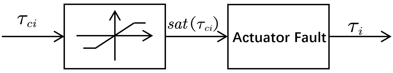
3.2. Actuator Model

As shown in Figure 2, The actuator of the USV exhibits saturation and faults. Where ${\mathit{\tau }}_c$ represents the control input, and $\mathit{\tau }$ represents the actuator output. The saturation of the actuator can be expressed as

$$sat\left({\tau }_{ci}\right)={\tau }_{ci}+{\nabla }_i=\left\{\begin{array}{c}{\tau }_{cimax}{\tau }_{ci}\ge {\tau }_{cimax};\hfill \\ {\tau }_{ci}{\tau }_{cimax}\ge {\tau }_{ci}\ge {\tau }_{cimin};\hfill \\ {\tau }_{cimin}{\tau }_{ci}\le {\tau }_{cimin};\hfill \end{array}\right.$$

(7)

where $i=u,r$, ${\tau }_{cimax}$ and ${\tau }_{cimin}$ represent the upper and lower limits of the actuator’s output and ${\nabla }_i$ denotes the unexecuted portion.

The fault model of the thruster can be denoted as

$${\tau }_u={\sigma }_{u}sat\left({\tau }_{cu}\right)+{\overline{\tau }}_u$$

(8)

$${\tau }_r={\sigma }_{r}sat\left({\tau }_{cr}\right)+{\overline{\tau }}_r$$

(9)

where ${\sigma }_u$ and ${\sigma }_r$ are the thruster effectiveness loss proportional constant, and ${\overline{\tau }}_u$ and ${\overline{\tau }}_r$ are fault bias values. The following assumptions are made for thruster failure.

Assumption 2.

Based on the physical properties of the controller itself, the deviation of the control mechanism is a bounded quantity, and there exist two constants ${\overline{\tau }}_u^{*}$ and ${\overline{\tau }}_r^{*}$ that satisfy ${\overline{\tau }}_u\le {\overline{\tau }}_u^{*}$ and ${\overline{\tau }}_r\le {\overline{\tau }}_r^{*}$, respectively.

Assumption 3.

Based on scenarios in actual engineering, it is assumed that the propellers do not exist in a state of complete failure or stuckness, i.e., ${\tau }_{cu}\ne 0$ and ${\tau }_{cr}\ne 0$, and the failure coefficients are denoted as bounded quantities that satisfy $0<{\tau }_{cu}\le 1$ and $0<{\tau }_{cu}\le 1$.

The failure modes considered are shown in

Table 1. Fault types of each thruster ($i=u,r$).

Fault Model	${\mathit{\sigma }}_{\mathit{i}}$	$\overline{{\mathit{\tau }}_{\mathit{i}}}$
Normal	${\sigma }_i=1$	$\overline{{\tau }_i}=0$
Loss of effectiveness	$0<{\sigma }_i<1$	$\overline{{\tau }_i}=0$
Increased bias input	${\sigma }_i=1$	$\overline{{\tau }_i}\ne 0$
Both faults occur	$0<{\sigma }_i<1$	$\overline{{\tau }_i}\ne 0$

.

4. Adaptive Control Law Design

In this section, the backstepping method is first used to design the virtual control volume, which is the desired USV speed, and then the adaptive controller is designed in conjunction with the terminal sliding mode to make the ship tolerant to propeller faults while performing path tracking. Additionally, the correctness of the designed controller is proved according to Lyapunov stability theory.

4.1. Virtual Control Law Design

Assumption 4.

The reference trajectory $\left(x_d,y_d\right)$ of the USV is smooth and has first and second-order derivatives.

The position tracking error is defined as

$$\left[\begin{array}{c}{x}_e\\ y_e\end{array}\right]=\left[\begin{array}{c}x-x_d\\ y-y_d\end{array}\right]$$

(10)

The derivation can be obtained:

$$\left[\begin{array}{c}{\dot{x}}_e\\ {\dot{y}}_e\end{array}\right]=\left[\begin{array}{cc}cos\left(\psi \right)& -sin\left(\psi \right)\\ sin\left(\psi \right)& cos\left(\psi \right)\end{array}\right]\left[\begin{array}{c}u\\ v\end{array}\right]-\left[\begin{array}{c}{\dot{x}}_d\\ {\dot{y}}_d\end{array}\right]$$

(11)

In order to make these errors converge to zero, the virtual control law is designed to be

$$\left[\begin{array}{c}{u}_d\\ v_d\end{array}\right]=\left[\begin{array}{cc}cos\left(\psi \right)& sin\left(\psi \right)\\ -sin\left(\psi \right)& cos\left(\psi \right)\end{array}\right]\left[\begin{array}{c}{\dot{x}}_d-{\displaystyle \frac{k{x}_e}{\sqrt{x_e+y_e+c}}}\\ {\dot{y}}_d-{\displaystyle \frac{k{y}_e}{\sqrt{x_e+y_e+c}}}\end{array}\right]$$

(12)

where $k>0$, $c>0$. Let $u_e=u-u_d$, $v_e=v-v_d$, so Equation (11) can be expressed as:

$$\left[\begin{array}{c}{\dot{x}}_e\\ {\dot{y}}_e\end{array}\right]=\left[\begin{array}{cc}cos\left(\psi \right)& -sin\left(\psi \right)\\ sin\left(\psi \right)& cos\left(\psi \right)\end{array}\right]\left[\begin{array}{c}{u}_e+u_d\\ v_e+v_d\end{array}\right]-\left[\begin{array}{c}{\dot{x}}_d\\ {\dot{y}}_d\end{array}\right]$$

(13)

In order to facilitate subsequent expressions, let $\sqrt{x_e^2+y_e^2+c}=w$. Equation (11) can now be further expressed as

$$\left[\begin{array}{c}{\dot{x}}_e\\ {\dot{y}}_e\end{array}\right]=\left[\begin{array}{c}{\displaystyle \frac{-k{x}_e}{w}}\\ {\displaystyle \frac{-k{y}_e}{w}}\end{array}\right]+\left[\begin{array}{cc}cos\left(\psi \right)& -sin\left(\psi \right)\\ sin\left(\psi \right)& cos\left(\psi \right)\end{array}\right]\left[\begin{array}{c}{u}_e\\ v_e\end{array}\right]$$

(14)

Define the Lyapunov function as

$$V={\displaystyle \frac{1}{2}}{x}_e^2+{\displaystyle \frac{1}{2}}{y}_e^2$$

(15)

The derivation of the above equation can be obtained

$$\dot{V}=x_e{\dot{x}}_e+y_e{\dot{y}}_e=-{\displaystyle \frac{k}{w}}{x}_e^2-{\displaystyle \frac{k}{w}}{y}_e^2+\left[x_e,y_e\right]\left[\begin{array}{cc}cos\left(\psi \right)& -sin\left(\psi \right)\\ sin\left(\psi \right)& cos\left(\psi \right)\end{array}\right]\left[\begin{array}{c}{u}_e\\ v_e\end{array}\right]$$

(16)

when $u_e\to 0$ and $v_e\to 0$, the above equation can be equated to

$$\dot{V}=-{\displaystyle \frac{k}{w}}{x}_e^2-{\displaystyle \frac{k}{w}}{y}_e^2$$

(17)

The next step involves designing control law such that $u_e\to 0$, $v_e\to 0$.

In order to facilitate the subsequent statement, the derivative of the virtual control law is first obtained:

$$\left[\begin{array}{c}{\dot{u}}_d\\ {\dot{v}}_d\end{array}\right]=\left[\begin{array}{c}r{v}_d\\ -r{u}_d\end{array}\right]+\left[\begin{array}{cc}cos\psi & sin\psi \\ -sin\psi & cos\psi \end{array}\right]\left[\begin{array}{c}{\ddot{x}}_d-k(w^{-1}-w^{-3}{x}_e^2){\dot{x}}_e+k{w}^{-3}{x}_e{y}_e{\dot{y}}_e\\ {\ddot{y}}_d-k(w^{-1}-w^{-3}{y}_e^2){\dot{y}}_e+k{w}^{-3}{x}_e{y}_e{\dot{x}}_e\end{array}\right]$$

(18)

4.2. Surge Adaptive Control Law Design

Considering the unmodeled dynamics in the system, the dynamic model of the USV can be expressed as

$$\left\{\begin{array}{c}\dot{u}={\displaystyle \frac{1}{m_{11}}}\left(m_{22}vr-d_{11}u-f_u+{\tau }_{wu}+{\tau }_u\right)\hfill \\ \dot{v}={\displaystyle \frac{1}{m_{22}}}\left(-m_{11}ur-d_{22}v-f_v+{\tau }_{wv}\right)\hfill \\ \dot{r}={\displaystyle \frac{1}{m_{33}}}\left[\left(m_{11}-m_{22}\right)uv-d_{33}r-f_r+{\tau }_{wr}+{\tau }_r\right]\hfill \end{array}\right.$$

(19)

The fast terminal sliding mode is constructed as

$$S_1={\dot{u}}_e+{\alpha }_{u0}{u}_e+{\beta }_{u0}{u}_e^{q_{u0}/p_{u0}}$$

(20)

where ${\alpha }_{u_0}>0$, ${\beta }_{u0}>0$, $q_{u0}$ and $p_{u0}\left(q_{u0}<p_{u0}\right)$ are odd numbers.

Expanding the above equation yields

$$\begin{gathered} S_1={\dot{u}}_e+{\alpha }_{u0}{u}_e+{\beta }_{u0}{u}_e^{q_{u0}/p_{u0}} \\ =\left(\dot{u}-{\dot{u}}_d\right)+{\alpha }_{u0}{u}_e+{\beta }_{u0}{u}_e^{q_{u0}/p_{u0}} \\ ={\displaystyle \frac{1}{m_{11}}}\left(m_{22}vr-d_{11}u-f_u+{\tau }_u+{\tau }_{wu}\right)-{\dot{u}}_d+{\alpha }_{u0}{u}_e+{\beta }_{u0}{u}_e^{q_{u0}/p_{u0}} \\ ={\displaystyle \frac{1}{m_{11}}}\left(m_{22}vr-d_{11}u\right)-{\dot{u}}_d+{\displaystyle \frac{1}{m_{11}}}\left({\tau }_{wu}-f_u\right)+{\displaystyle \frac{1}{m_{11}}}{\tau }_u+{\alpha }_{u0}{u}_e+{\beta }_{u0}{u}_e^{q_{u0}/p_{u0}} \\ ={△}_u+{\displaystyle \frac{1}{m_{11}}}\left({\tau }_{wu}-f_u\right)+{\displaystyle \frac{1}{m_{11}}}{\tau }_u+{\alpha }_{u0}{u}_e+{\beta }_{u0}{u}_e^{q_{u0}/p_{u0}} \end{gathered}$$

(21)

where

$${△}_u={\displaystyle \frac{1}{m_{11}}}\left(m_{22}vr-d_{11}u\right)-{\dot{u}}_d$$

When $S_1=0$, $u_e$ can approach 0, so the surge adaptive control law is designed as

$$\begin{array}{c}\hfill {\tau }_u=-\left({\tau }_{wu}-f_u\right)-m_{11}{△}_u-m_{11}\left({\alpha }_{u0}{u}_e+{\beta }_{u0}{u}_e^{q_{u0}/p_{u0}}\right)\end{array}$$

(22)

let

$$\alpha =m_{11}{△}_u+m_{11}\left({\alpha }_{u0}{u}_e+{\beta }_{u0}{u}_e^{q_{u0}/p_{u0}}\right)$$

thus, Equation (22) can be expressed as

$${\tau }_u=-\left({\tau }_{wu}-f_u\right)-\alpha$$

(23)

From Equation (8), it can be observed that

$${\tau }_{cu}=-{\displaystyle \frac{1}{{\sigma }_u}}\alpha -{\displaystyle \frac{1}{{\sigma }_u}}\left({\tau }_{wu}-f_u+{\overline{\tau }}_u\right)-{\nabla }_u=-k_u\alpha -d_u$$

(24)

where

$$\left\{\begin{array}{c}{d}_u={\displaystyle \frac{1}{{\sigma }_u}}\left({\tau }_{wu}-f_u+{\overline{\tau }}_u\right)+{\nabla }_{ u}\hfill \\ {\sigma }_u{k}_u=1\hfill \end{array}\right.$$

Remark 1.

Since it has been assumed that ${\sigma }_u\ne 0$, $k_u$ is a bounded quantity, and $k_u^{*}\ge \left|k_u\right|$.

Since $k_u$ and $d_u$ are unknown and varying, so Equation (24) is written as follows:

$${\tau }_{uc}=-{\widehat{k}}_u\alpha -{\widehat{d}}_u$$

(25)

According to the universal approximation property of RBF neural networks, the neural network output expression for the unknown term $d_u$ is

$$d_u={\mathit{W}}_u^{*\mathrm{T}}\mathit{h}\left(\mathit{z}\right)+{\epsilon }_u$$

(26)

$${\widehat{d}}_u={\widehat{\mathit{W}}}_u^{\mathrm{T}}\mathit{h}\left(\mathit{z}\right)$$

(27)

where ${\mathit{W}}_u^{*}$ is the network ideal weights, ${\widehat{\mathit{W}}}_u$ is an estimate of ${\mathit{W}}_u^{*}$, and $\mathit{z}={\left[u,v,r\right]}^{\mathrm{T}}$ is the input to the network. ${\epsilon }_u$ is the neural network approximation error and satisfies $\left|{\epsilon }_u\right|\le {\epsilon }_u^{*}$.

The adaptive control law is designed as

$$\left\{\begin{array}{c}{\dot{\widehat{k}}}_u={\gamma }_{u1}\left(u_e\alpha -g_{u1}{\widehat{k}}_u\right)\hfill \\ {\dot{\widehat{\mathit{W}}}}_{\mathbf{u}}={\gamma }_{u2}\left(u_e\mathit{h}\left(\mathit{z}\right)-g_{u2}{\widehat{\mathit{W}}}_{\mathbf{u}}\right)\hfill \end{array}\right.$$

(28)

where ${\gamma }_{u1}$, ${\gamma }_{u2}$, $g_{u1}$, and $g_{u2}$ are all greater than 0.

The following Lyapunov function is chosen for stability analysis, where ${\tilde{\mathit{W}}}_u={\mathit{W}}_u^{*}-{\widehat{\mathit{W}}}_u$ and ${\tilde{k}}_u=k_u-{\widehat{k}}_u$.

$$V_1={\displaystyle \frac{1}{2}}{m}_{11}{u}_e^2+{\displaystyle \frac{{\sigma }_u}{2{\gamma }_{u1}}}{\tilde{k}}_u^2+{\displaystyle \frac{{\sigma }_u}{2{\gamma }_{u2}}}{\tilde{\mathit{W}}}_u^{\mathrm{T}}{\tilde{\mathit{W}}}_u$$

(29)

The derivative of $V_1$ is

$$\begin{array}{cc}\hfill & {\dot{V}}_1=m_{11}{u}_e{\dot{u}}_e-{\displaystyle \frac{{\sigma }_u}{{\gamma }_{u1}}}{\tilde{k}}_u{\dot{\widehat{k}}}_u-{\displaystyle \frac{{\sigma }_u}{{\gamma }_{u2}}}{\tilde{\mathit{W}}}_u^{\mathrm{T}}{\dot{\widehat{\mathit{W}}}}_u\hfill \\ \hfill & =u_e\left({\tau }_u+\left({\tau }_{wu}-f_u\right)+m_{11}{△}_u\right)-{\displaystyle \frac{{\sigma }_u}{{\gamma }_{u1}}}{\tilde{k}}_u{\dot{\widehat{k}}}_u-{\displaystyle \frac{{\sigma }_u}{{\gamma }_{u2}}}{\tilde{\mathit{W}}}_u^{\mathrm{T}}{\dot{\widehat{\mathit{W}}}}_u\hfill \\ \hfill & =u_e\left[{\sigma }_u\left({\tau }_{cu}+{\nabla }_u\right)+{\overline{\tau }}_u+\left({\tau }_{wu}-f_u\right)+\alpha \right]\hfill \\ \hfill & -u_e{m}_{11}\left({\alpha }_{u0}{u}_e+{\beta }_{u0}{u}_e^{q_{u0}/p_{u0}}\right)-{\displaystyle \frac{{\sigma }_u}{{\gamma }_{u1}}}{\tilde{k}}_u{\dot{\widehat{k}}}_u-{\displaystyle \frac{{\sigma }_u}{{\gamma }_{u2}}}{\tilde{\mathit{W}}}_u^{\mathrm{T}}{\dot{\widehat{\mathit{W}}}}_u\hfill \\ \hfill & =u_e\left[-{\sigma }_u{\widehat{k}}_u\alpha -{\sigma }_u{\widehat{d}}_u+\left({\tau }_{wu}-f_u+{\overline{\tau }}_u\right)+{\sigma }_u{\nabla }_u+\alpha \right]\hfill \\ \hfill & -u_e{m}_{11}\left({\alpha }_{u0}{u}_e+{\beta }_{u0}{u}_e^{q_{u0}/p_{u0}}\right)-{\displaystyle \frac{{\sigma }_u}{{\gamma }_{u1}}}{\tilde{k}}_u{\dot{\widehat{k}}}_u-{\displaystyle \frac{{\sigma }_u}{{\gamma }_{u2}}}{\tilde{\mathit{W}}}_u^{\mathrm{T}}{\dot{\widehat{\mathit{W}}}}_u\hfill \\ \hfill & =u_e\left[-{\sigma }_u{\widehat{k}}_u\alpha +{\sigma }_u{k}_u\alpha -{\sigma }_u{\widehat{d}}_u+\sigma d_u\right]\hfill \\ \hfill & -u_e{m}_{11}\left({\alpha }_{u0}{u}_e+{\beta }_{u0}{u}_e^{q_{u0}/p_{u0}}\right)-{\displaystyle \frac{{\sigma }_u}{{\gamma }_{u1}}}{\tilde{k}}_u{\dot{\widehat{k}}}_u-{\displaystyle \frac{{\sigma }_u}{{\gamma }_{u2}}}{\tilde{\mathit{W}}}_u^{\mathrm{T}}{\dot{\widehat{\mathit{W}}}}_u\hfill \\ \hfill & =u_e\left[{\sigma }_u\alpha {\tilde{k}}_u+{\mathit{W}}_u^T\mathit{h}\left(z\right)+{\epsilon }_u\right]-u_e{m}_{11}\left({\alpha }_{u0}{u}_e+{\beta }_{u0}{u}_e^{q_{u0}/p_{u0}}\right)-{\displaystyle \frac{{\sigma }_u}{{\gamma }_{u1}}}{\tilde{k}}_u{\dot{\widehat{k}}}_u-{\displaystyle \frac{{\sigma }_u}{{\gamma }_{u2}}}{\tilde{\mathit{W}}}_u^{\mathrm{T}}{\dot{\widehat{\mathit{W}}}}_u\hfill \\ \hfill & =-u_e{m}_{11}\left({\alpha }_{u0}{u}_e+{\beta }_{u0}{u}_e^{q_{u0}/p_{u0}}\right)+u_e\left[{\sigma }_u\alpha {\tilde{k}}_u+{\mathit{W}}_u^T\mathit{h}\left(z\right)+{\epsilon }_u\right]\hfill \\ \hfill & -{\sigma }_u{\tilde{k}}_u\left(u_e\alpha -g_{u1}{\widehat{k}}_u\right)-{\sigma }_u{\tilde{\mathit{W}}}_u^{\mathrm{T}}\left(u_e\mathit{h}\left(z\right)-g_{u2}{\widehat{\mathit{W}}}_u\right)\hfill \\ \hfill & =-u_e{m}_{11}\left({\alpha }_{u0}{u}_e+{\beta }_{u0}{u}_e^{q_{u0}/p_{u0}}\right)+u_e{\epsilon }_u+{\sigma }_u{g}_{u1}{\tilde{k}}_u{\widehat{k}}_u+{\sigma }_u{g}_{u2}{\tilde{\mathit{W}}}_u^{\mathrm{T}}{\widehat{\mathit{W}}}_u\hfill \end{array}$$

(30)

Because of

$$\begin{array}{cc}\hfill & 2{\tilde{k}}_u{\widehat{k}}_u=\left(k_u-{\widehat{k}}_u\right){\widehat{k}}_u+{\tilde{k}}_u\left(k_u-{\tilde{k}}_u\right)\hfill \\ \hfill & =k_u{\widehat{k}}_u-{\widehat{k}}_u{\widehat{k}}_u+{\tilde{k}}_u{k}_u-{\tilde{k}}_u{\tilde{k}}_u\hfill \\ \hfill & =k_u\left(k_u-{\tilde{k}}_u\right)-{\widehat{k}}_u{\widehat{k}}_u+{\tilde{k}}_u{k}_u-{\tilde{k}}_u{\tilde{k}}_u\hfill \\ \hfill & =k_u{k}_u-k_u{\tilde{k}}_u-{\widehat{k}}_u{\widehat{k}}_{u1}+{\tilde{k}}_{u1}{k}_{u1}-{\tilde{k}}_{u1}{\tilde{k}}_{u1}\hfill \\ \hfill & =k_u^2-{\widehat{k}}_u^2-{\tilde{k}}_u^2\hfill \\ \hfill & =k_u^2-{\tilde{k}}_u^2\hfill \\ \hfill & \le k_u^{*2}-{\tilde{k}}_u^2\hfill \end{array}$$

(31)

$${\sigma }_u{g}_{u1}{\tilde{k}}_u{\widehat{k}}_u\le g_{u1}{\tilde{k}}_u{\widehat{k}}_u\le -{\displaystyle \frac{1}{2}}{g}_{u1}{\tilde{k}}_u^2+{\displaystyle \frac{1}{2}}{g}_{u1}{k}_u^{*2}$$

(32)

The same reasoning leads to

$${\sigma }_u{g}_{u2}{\tilde{\mathit{W}}}_u^{\mathrm{T}}{\widehat{\mathit{W}}}_u\le g_{u2}{\tilde{\mathit{W}}}_u^{\mathrm{T}}{\widehat{\mathit{W}}}_u\le -{\displaystyle \frac{1}{2}}{g}_{u2}{\tilde{\mathit{W}}}_u^{\mathrm{T}}{\tilde{\mathit{W}}}_u+{\displaystyle \frac{1}{2}}{g}_{u2}{\mathit{W}}_u^{*\mathrm{T}}{\mathrm{W}}_u^{*}$$

(33)

Applying Young’s inequality gives

$$u_e{\sigma }_u{\epsilon }_u\le \left|u_e\right|{\epsilon }_u^{*}\le {\displaystyle \frac{1}{2}}{\epsilon }_u^{*2}+{\displaystyle \frac{1}{2}}{u}_e^2$$

(34)

Therefore, Equation (30) can be expressed as

$$\begin{array}{cc}\hfill & {\dot{V}}_1\le -\left(m_{11}{\alpha }_{u0}-{\displaystyle \frac{1}{2}}\right)u_e^2-m_{11}{\beta }_{u0}{u}_e^{q_{u0}/p_{u0}+1}-{\displaystyle \frac{1}{2}}{g}_{u1}{\tilde{k}}_u^2-{\displaystyle \frac{1}{2}}{g}_{u2}{\tilde{\mathit{W}}}_u^{\mathrm{T}}{\tilde{\mathit{W}}}_u\hfill \\ \hfill & +{\displaystyle \frac{1}{2}}{g}_{u1}{k}_u^{*2}+{\displaystyle \frac{1}{2}}{g}_{u2}{\mathit{W}}_u^{*\mathrm{T}}{\mathit{W}}_u^{*}+{\displaystyle \frac{1}{2}}{\epsilon }_u^{*2}\hfill \\ \hfill & \le -\left(m_{11}{\alpha }_{u0}-{\displaystyle \frac{1}{2}}\right)u_e^2-{\displaystyle \frac{1}{2}}{g}_{u1}{\tilde{k}}_u^2-{\displaystyle \frac{1}{2}}{g}_{u2}{\tilde{\mathit{W}}}_u^{\mathrm{T}}{\tilde{\mathit{W}}}_u\hfill \\ \hfill & +{\displaystyle \frac{1}{2}}{g}_{u1}{k}_u^{*2}+{\displaystyle \frac{1}{2}}{g}_{u2}{\mathit{W}}_u^{*\mathrm{T}}{\mathit{W}}_u^{*}+{\displaystyle \frac{1}{2}}{\epsilon }_u^{*2}\hfill \\ \hfill & \le -C_u{V}_1+U_u\hfill \end{array}$$

(35)

where

$$\left\{\begin{array}{c}{C}_u=2min\left(m_{11}{\alpha }_{u0}-{\displaystyle \frac{1}{2}},{\displaystyle \frac{1}{2}}{g}_{u1},{\displaystyle \frac{1}{2}}{g}_{u2}\right)\hfill \\ U_u={\displaystyle \frac{1}{2}}{\epsilon }_u^{*2}+{\displaystyle \frac{1}{2}}{g}_{u1}{k}_u^{*2}+{\displaystyle \frac{1}{2}}{g}_u{\mathit{W}}_u^{*\mathrm{T}}{\mathit{W}}_u^{*}\hfill \end{array}\right.$$

As obtained from Equation (35):

$$0\le V_1\le {\displaystyle \frac{U_u}{C_u}}+\left(V_1\left(0\right)-{\displaystyle \frac{U_u}{C_u}}\right)e^{-C_{u}t}$$

(36)

From Equation (36), it is known that $V_1$ is convergent, and thus $u_e$ is bounded.

4.3. Steering Torque Adaptive Control Law Design

A fast terminal sliding model with a recursive structure is as follows:

$$\left\{\begin{array}{c}{S}_1={\dot{v}}_e+{\alpha }_{r0}{v}_e+{\beta }_{r0}{v}_e^{q_{r0}/p_{r0}}\hfill \\ S_2={\dot{S}}_1+{\alpha }_{r1}{S}_1+{\beta }_{r1}{S}_1^{q_{r1}/p_{r1}}\hfill \end{array}\right.$$

(37)

where ${\alpha }_{r0}>0$, ${\alpha }_{r1}>0$, ${\beta }_{r0}>0$, ${\beta }_{r1}>0$ and $q_{r0}$, $p_{r0}$, $q_{r1}$, and $q_{r1}\left(q_{r0}<p_{r0},q_{r1}<p_{r1}\right)$ are odd numbers. Expanding $S_2$ to obtain

$$S_2={\ddot{v}}_e+{\alpha }_{r0}{\dot{v}}_e+{\beta }_{r0}{\displaystyle \frac{q_{r0}}{p_{r0}}}{v}_e^{q_{r0}/p_{r0}-1}{\dot{v}}_e+{\alpha }_{r1}{S}_1+{\beta }_{r1}{S}_1^{q_{r1}/p_{r1}}$$

(38)

To achieve $v_e\to 0$, $S_2$ must be set to zero for the design of the steering torque control law. It is first necessary to expand ${\ddot{v}}_e$:

$${\ddot{v}}_e=\ddot{v}-{\ddot{v}}_d$$

(39)

The next step is to calculate $\ddot{v}$ and ${\ddot{v}}_d$ separately. From Equation (19), it follows that

$$\begin{array}{cc}\hfill & \ddot{v}={\displaystyle \frac{1}{m_{22}}}\left[-m_{11}\dot{u}r-m_{11}u\dot{r}-d_{22}\dot{v}+\left({\dot{\tau }}_{wv}-{\dot{f}}_v\right)\right]\hfill \\ \hfill & ={\displaystyle \frac{1}{m_{22}}}\left[-m_{11}\dot{u}r-d_{22}\dot{v}+\left({\dot{\tau }}_{wv}-{\dot{f}}_v\right)\right]\hfill \\ & -{\displaystyle \frac{m_{11}u}{m_{22}}}\left[{\displaystyle \frac{m_{11}-m_{22}}{m_{33}}}uv-{\displaystyle \frac{d_{33}}{m_{33}}}r+{\displaystyle \frac{1}{m_{33}}}\left({\tau }_{wr}-f_r\right)+{\displaystyle \frac{1}{m_{33}}}{\tau }_r\right]\hfill \\ \hfill & =\left({\displaystyle \frac{1}{m_{22}{m}_{33}}}\right)\left[-m_{33}{m}_{11}\dot{u}r-m_{33}{d}_{22}\dot{v}+m_{33}\left({\dot{\tau }}_{wv}-{\dot{f}}_v\right)\right]\hfill \\ & -{\displaystyle \frac{m_{11}u}{m_{22}{m}_{33}}}\left[\left(m_{11}-m_{22}\right)uv-d_{33}r+\left({\tau }_{wr}-f_r\right)+{\tau }_r\right]\hfill \end{array}$$

(40)

From Equation (18), it follows that

$$\begin{gathered} {\dot{v}}_d=-r{v}_d-sin\left(\psi \right)\left[{\ddot{x}}_d-k\left(w^{-1}-w^{-3}{x}_e^2\right){\dot{x}}_e+k{w}^{-3}{x}_e{y}_e{\dot{y}}_e\right] \\ +cos\left(\psi \right)\left[{\ddot{y}}_d-k\left(w^{-1}-w^{-3}{y}_e^2\right){\dot{y}}_e+k{w}^{-1}{x}_e{y}_e{\dot{x}}_e\right] \end{gathered}$$

(41)

Let

$$f=-sin\left(\psi \right)\left[{\ddot{x}}_d-k\left(w^{-1}-w^{-3}{x}_e^2\right){\dot{x}}_e+k{w}^{-3}{x}_e{y}_e{\dot{y}}_e\right]$$

$$+cos\left(\psi \right)\left[{\ddot{y}}_d-k\left(w^{-1}-w^{-3}{y}_e^2\right){\dot{y}}_e+k{w}^{-1}{x}_e{y}_e{\dot{x}}_e\right]$$

then,

$${\dot{v}}_d=-r{v}_d+f$$

(42)

Continuing the derivation for ${\dot{v}}_d$ leads to

$${\ddot{v}}_d=-\dot{r}{v}_d-r{\dot{v}}_d+\dot{f}=-{\displaystyle \frac{v_d}{m_{33}}}\left[\left(m_{11}-m_{22}\right)uv-d_{33}r+\left({\tau }_{wr}-f_r\right)+{\tau }_r\right]-r{\dot{v}}_d+\dot{f}$$

(43)

Therefore, ${\ddot{v}}_e$ can be obtained from Equations (40) and (43):

$${\ddot{v}}_e=\ddot{v}-{\ddot{v}}_d={\displaystyle \frac{1}{m_{22}{m}_{33}}}\left[b\left({\tau }_r+{\tau }_{wr}-f_r\right)+m_{33}\left({\dot{\tau }}_{wv}-{\dot{f}}_v\right)+h\right]$$

(44)

where

$$\begin{array}{cc}\hfill h=& m_{22}{v}_d\left(\left(m_{11}-m_{22}\right)uv-d_{33}r\right)+m_{22}{m}_{33}\left(r{\dot{v}}_d-\dot{f}\right)\hfill \\ \hfill & -d_{22}{m}_{33}\dot{v}-m_{11}{m}_{33}\dot{u}r+m_{11}{d}_{33}ur+m_{11}\left(m_{22}-m_{11}\right)u^{2}v\hfill \end{array}$$

(45)

$$b=m_{22}{v}_d-m_{11}u$$

(46)

The following result is obtained from Equations (38)–(46):

$${\tau }_r=-\left({\tau }_{wr}-f_r\right)-{\displaystyle \frac{m_{33}}{b}}\left({\dot{\tau }}_{wv}-{\dot{f}}_v\right)-{\displaystyle \frac{m_{22}{m}_{33}}{b}}\left({△}_r+{\alpha }_{r1}{S}_1+{\beta }_{r1}{S}_1^{q_{r1}/p_{r1}}\right)$$

(47)

where

$${△}_r={\displaystyle \frac{1}{m_{22}{m}_{33}}}h+{\alpha }_{r0}{\dot{v}}_e+{\beta }_{r0}{\displaystyle \frac{q_{r0}}{p_{r0}}}{v}_e^{q_{r0}/p_{r0}-1}{\dot{v}}_e$$

Remark 2.

For most conventional surface vessels, the inertia parameter $m_{11}$ is 20% larger than $m_{22}$, and, therefore, $b>0$. Then, no singular values will occur.

Remark 3.

Since $v_d$ and u were proved to be bounded earlier, b is bounded. Let the upper bound of b be $b^{*}$.

Let

$$\beta ={\displaystyle \frac{m_{22}{m}_{33}}{b}}\left({△}_r+{\alpha }_{r1}{S}_1+{\beta }_{r1}{S}_1^{q_{r1}/p_{r1}}\right)$$

that

$${\tau }_r=-\left({\tau }_{wr}-f_r\right)-{\displaystyle \frac{m_{33}}{b}}\left({\dot{\tau }}_{wv}-{\dot{f}}_v\right)-\beta$$

(48)

From Equation (9), it can be concluded that

$$\begin{array}{cc}\hfill & {\tau }_{cr}=-{\displaystyle \frac{1}{{\sigma }_r}}\beta -{\displaystyle \frac{1}{{\sigma }_r}}\left[\left({\tau }_{wr}-f_r\right)+{\displaystyle \frac{m_{33}}{b}}\left({\dot{\tau }}_{wv}-{\dot{f}}_v\right)+{\overline{\tau }}_r\right]-{\nabla }_r\hfill \\ \hfill & =-k_r\beta -d_r\hfill \end{array}$$

(49)

where

$$\left\{\begin{array}{c}{d}_r={\displaystyle \frac{1}{{\sigma }_r}}\left[\left({\tau }_{wr}-f_r\right)+{\displaystyle \frac{m_{33}}{b}}\left({\dot{\tau }}_{wv}-{\dot{f}}_v\right)+{\overline{\tau }}_r\right]+{\nabla }_{ r}\hfill \\ {\sigma }_r{k}_r=1\hfill \end{array}\right.$$

Remark 4.

Since it has been assumed that ${\sigma }_r\ne 0$, $k_u$ is a bounded quantity, and $k_r^{*}\ge \left|k_r\right|$.

Since $k_u$ and $d_u$ are unknown and varying, so Equation (49) is written as follows:

$${\tau }_{cr}=-{\widehat{k}}_r\beta -{\widehat{d}}_r$$

(50)

According to the universal approximation property of RBF neural networks, the neural network output expression for the unknown term $d_r$ is

$$d_r={\mathit{W}}_r^{*\mathrm{T}}\mathit{h}\left(\mathit{z}\right)+{\epsilon }_r$$

(51)

$${\widehat{d}}_r={\widehat{\mathit{W}}}_r^{\mathrm{T}}\mathit{h}\left(\mathit{z}\right)$$

(52)

where ${\mathit{W}}_r^{*}$ is the network ideal weights, ${\widehat{\mathit{W}}}_r$ is an estimate of ${\mathit{W}}_r^{*}$, and $\mathit{z}={\left[u,v,r\right]}^{\mathrm{T}}$ is the input to the network. ${\epsilon }_r$ is the neural network approximation error and satisfies $\left|{\epsilon }_r\right|<{\epsilon }_r^{*}$.

The adaptive control law is designed as

$$\left\{\begin{array}{c}{\dot{\widehat{k}}}_r={\gamma }_{r1}\left(b{S}_1\beta -g_{r1}{\widehat{k}}_{r1}\right)\hfill \\ {\dot{\widehat{\mathit{W}}}}_r={\gamma }_{r2}\left(b{S}_1\mathit{h}\left(\mathit{z}\right)-g_{r2}{\widehat{\mathit{W}}}_r\right)\hfill \end{array}\right.$$

(53)

where ${\gamma }_{r1}$, ${\gamma }_{r2}$, $g_{r1}$ and $g_{r2}$ are all greater than 0.

The following Lyapunov function is chosen for stability analysis, where ${\tilde{\mathit{W}}}_r={\mathit{W}}_r^{*}-{\widehat{\mathit{W}}}_r$ and ${\tilde{k}}_r=k_r-{\widehat{k}}_r$:

$$V_2={\displaystyle \frac{1}{2}}{m}_{22}{m}_{33}{S}_1^2+{\displaystyle \frac{{\sigma }_r}{2{\gamma }_{r1}}}{\tilde{k}}_r^2+{\displaystyle \frac{{\sigma }_r}{2{\gamma }_{r2}}}{\tilde{\mathit{W}}}_r^{\mathrm{T}}{\tilde{\mathit{W}}}_r$$

(54)

The derivative of $V_2$ is

$$\begin{array}{cc}\hfill & {\dot{V}}_2=m_{22}{m}_{33}{S}_1{\dot{S}}_1-{\displaystyle \frac{{\sigma }_r}{{\gamma }_{r1}}}{\tilde{k}}_r{\dot{\widehat{k}}}_r-{\displaystyle \frac{{\sigma }_r}{{\gamma }_{r2}}}{\tilde{\mathit{W}}}_r^{\mathrm{T}}{\dot{\widehat{\mathit{W}}}}_r\hfill \\ \hfill & =m_{22}{m}_{33}{S}_1\left({\ddot{v}}_e+{\alpha }_{r0}{\dot{v}}_e+{\beta }_{r_0}{\displaystyle \frac{q_{r0}}{p_{r0}}}{v}_e^{q_{r0}/p_{r0}-1}{\dot{v}}_e\right)-{\displaystyle \frac{{\sigma }_r}{{\gamma }_{r1}}}{\tilde{k}}_r{\dot{\widehat{k}}}_r-{\displaystyle \frac{{\sigma }_r}{{\gamma }_{r2}}}{\tilde{\mathit{W}}}_r^{\mathrm{T}}{\dot{\widehat{\mathit{W}}}}_r\hfill \\ \hfill & =S_1\left[b\left({\tau }_r+{\tau }_{wr}-f_r\right)+m_{33}\left({\dot{\tau }}_{wv}-{\dot{f}}_v\right)+m_{22}{m}_{33}{△}_r\right]\hfill \\ \hfill & -{\displaystyle \frac{{\sigma }_r}{{\gamma }_{r1}}}{\tilde{k}}_r{\dot{\widehat{k}}}_r-{\displaystyle \frac{{\sigma }_r}{{\gamma }_{r2}}}{\tilde{\mathit{W}}}_r^{\mathrm{T}}{\dot{\widehat{\mathit{W}}}}_r\hfill \\ \hfill & =S_1\left[b{\sigma }_r{\tau }_{cr}+b{\sigma }_r{\nabla }_r+b{\overline{\tau }}_r+b\left({\tau }_{wr}-f_r\right)+m_{33}\left({\dot{\tau }}_{wv}-{\dot{f}}_v\right)+m_{22}{m}_{33}{△}_r\right]\hfill \\ \hfill & -{\displaystyle \frac{{\sigma }_r}{{\gamma }_{r1}}}{\tilde{k}}_r{\dot{\widehat{k}}}_r-{\displaystyle \frac{{\sigma }_r}{{\gamma }_{r2}}}{\tilde{\mathit{W}}}_r^{\mathrm{T}}{\dot{\widehat{\mathit{W}}}}_r\hfill \\ \hfill & =S_1\left[b{\sigma }_r\left(-{\widehat{k}}_r\beta -{\widehat{d}}_r\right)+b{\sigma }_r{\nabla }_r+b{\overline{\tau }}_r+b\left({\tau }_{wr}-f_r\right)+m_{33}\left({\dot{\tau }}_{wv}-{\dot{f}}_v\right)+m_{22}{m}_{33}{△}_r\right]\hfill \\ \hfill & -{\displaystyle \frac{{\sigma }_r}{{\gamma }_{r1}}}{\tilde{k}}_r{\dot{\widehat{k}}}_r-{\displaystyle \frac{{\sigma }_r}{{\gamma }_{r2}}}{\tilde{\mathit{W}}}_r^{\mathrm{T}}{\dot{\widehat{\mathit{W}}}}_r\hfill \\ \hfill & =S_1\left[-b{\sigma }_r{\widehat{k}}_r\beta -b{\sigma }_r{\widehat{d}}_r+b{\sigma }_r{\nabla }_r+b{\overline{\tau }}_r+b\left({\tau }_{wr}-f_r\right)+m_{33}\left({\dot{\tau }}_{wv}-{\dot{f}}_v\right)+m_{22}{m}_{33}{△}_r\right]\hfill \\ \hfill & -{\displaystyle \frac{{\sigma }_r}{{\gamma }_{r1}}}{\tilde{k}}_r{\dot{\widehat{k}}}_r-{\displaystyle \frac{{\sigma }_r}{{\gamma }_{r2}}}{\tilde{\mathit{W}}}_r^{\mathrm{T}}{\dot{\widehat{\mathit{W}}}}_r\hfill \\ \hfill & =S_1\left[-b{\sigma }_r{\widehat{k}}_r\beta -b{\sigma }_r{\widehat{d}}_r+b{\sigma }_r{d}_r+b{\sigma }_r{k}_r\beta -m_{22}{m}_{33}\left({\alpha }_{r0}{\dot{v}}_e+{\beta }_{r_0}{\displaystyle \frac{q_{r0}}{p_{r0}}}{v}_e^{q_{r0}/p_{r0}-1}{\dot{v}}_e\right)\right]\hfill \\ \hfill & -{\displaystyle \frac{{\sigma }_r}{{\gamma }_{r1}}}{\tilde{k}}_r{\dot{\widehat{k}}}_r-{\displaystyle \frac{{\sigma }_r}{{\gamma }_{r2}}}{\tilde{\mathit{W}}}_r^{\mathrm{T}}{\dot{\widehat{\mathit{W}}}}_r\hfill \\ \hfill & =S_1\left(b{\sigma }_r\beta {\tilde{k}}_r+b{\sigma }_r{\tilde{\mathit{W}}}_r^T\mathit{h}\left(\mathit{z}\right)+b{\sigma }_r{\epsilon }_r\right)-S_1{m}_{22}{m}_{33}\left({\alpha }_{r0}{\dot{v}}_e+{\beta }_{r_0}{\displaystyle \frac{q_{r0}}{p_{r0}}}{v}_e^{q_{r0}/p_{r0}-1}{\dot{v}}_e\right)\hfill \\ \hfill & -{\sigma }_r{\tilde{k}}_r\left(b{S}_1\beta -g_{r1}{\widehat{k}}_r\right)-{\sigma }_r{\tilde{\mathit{W}}}_r^T\left(b{S}_1\mathit{h}\left(\mathit{z}\right)-g_{r2}{\widehat{\mathit{W}}}_r\right)\hfill \\ \hfill & =-S_1{m}_{22}{m}_{33}\left({\alpha }_{r0}{\dot{v}}_e+{\beta }_{r_0}{\displaystyle \frac{q_{r0}}{p_{r0}}}{v}_e^{q_{r0}/p_{r0}-1}{\dot{v}}_e\right)+S_{1}b{\sigma }_r{\epsilon }_r\hfill \\ \hfill & +{\sigma }_r{g}_{r1}{\tilde{k}}_r{\widehat{k}}_r+{\sigma }_r{g}_{r2}{\tilde{W}}_r^T{\widehat{\mathit{W}}}_r\hfill \end{array}$$

(55)

From the previous analysis, it is clear that

$${\sigma }_r{g}_{r1}{\tilde{k}}_r{\widehat{k}}_r\le g_{r1}{\tilde{k}}_r{\widehat{k}}_r\le -{\displaystyle \frac{1}{2}}{g}_{r1}{\tilde{k}}_r^2+{\displaystyle \frac{1}{2}}{g}_{r1}{k}_r^{*2}$$

(56)

$${\sigma }_r{g}_{r2}{\tilde{\mathit{W}}}_r^{\mathrm{T}}{\widehat{\mathit{W}}}_r\le g_{r2}{\tilde{\mathit{W}}}_r^{\mathrm{T}}{\widehat{\mathit{W}}}_r\le -{\displaystyle \frac{1}{2}}{g}_{r2}{\tilde{\mathit{W}}}^{\mathrm{T}}\tilde{\mathit{W}}+{\displaystyle \frac{1}{2}}{g}_{r2}{\mathit{W}}^{*\mathrm{T}}{\mathit{W}}^{*}$$

(57)

$$S_{1}b{\sigma }_r{\epsilon }_r\le b^{*}\left|S_1\right|{\epsilon }_r^{*}\le {\displaystyle \frac{b^{*}}{2}}{\epsilon }_r^{*2}+{\displaystyle \frac{b^{*}}{2}}{S}_1^2$$

(58)

Therefore, Equation (55) can be denoted as

$$\begin{array}{cc}\hfill & {\dot{V}}_2\le -\left(m_{22}{m}_{33}{\alpha }_{r1}-{\displaystyle \frac{b^{*}}{2}}\right)S_1^2-m_{22}{m}_{33}{\beta }_{r1}{S}_1^{q_{r1}/p_{r1}+1}-{\displaystyle \frac{1}{2}}{g}_{r1}{\tilde{k}}_r^2-{\displaystyle \frac{1}{2}}{g}_{r2}{\tilde{\mathit{W}}}_r^{\mathrm{T}}\tilde{\mathit{W}}\hfill \\ \hfill & +{\displaystyle \frac{1}{2}}{g}_{r1}{k}_r^{*2}+{\displaystyle \frac{1}{2}}{g}_{r2}{\mathit{W}}_r^{*\mathrm{T}}{\mathit{W}}_{\mathbf{r}}^{*}+{\displaystyle \frac{b^{*}}{2}}{\epsilon }_u^{*2}\hfill \\ \hfill & \le -\left(m_{22}{m}_{33}{\alpha }_{r1}-{\displaystyle \frac{b^{*}}{2}}\right)S_1^2-{\displaystyle \frac{1}{2}}{g}_{r1}{\tilde{k}}_r^2-{\displaystyle \frac{1}{2}}{g}_{r2}{\tilde{\mathit{W}}}_r^{\mathrm{T}}{\tilde{\mathit{W}}}_r\hfill \\ \hfill & +{\displaystyle \frac{1}{2}}{g}_{r1}{k}_r^{*2}+{\displaystyle \frac{1}{2}}{g}_{r2}{\mathit{W}}_r^{*\mathrm{T}}{\mathit{W}}_{\mathbf{r}}^{*}+{\displaystyle \frac{b^{*}}{2}}{\epsilon }_u^{*2}\hfill \\ \hfill & \le -C_r{V}_2+U_r\hfill \end{array}$$

(59)

where

$$\left\{\begin{array}{c}{C}_r=2min\left(m_{22}{m}_{33}{\alpha }_{r1}-{\displaystyle \frac{b^{*}}{2}},{\displaystyle \frac{1}{2}}{g}_{r1},{\displaystyle \frac{1}{2}}{g}_{r2}\right)\hfill \\ U_r={\displaystyle \frac{1}{2}}{g}_{r1}{k}_r^{*2}+{\displaystyle \frac{1}{2}}{g}_{r2}{\mathit{W}}_r^{*\mathrm{T}}{\mathit{W}}_{\mathbf{r}}^{*}+{\displaystyle \frac{b^{*}}{2}}{\epsilon }_u^{*2}\hfill \end{array}\right.$$

As obtained from Equation (59):

$$0\le V_2\le {\displaystyle \frac{U_r}{C_r}}+\left(V_2\left(0\right)-{\displaystyle \frac{U_r}{C_r}}\right)e^{-C_{r}t}$$

(60)

Equation (60) shows the convergence of $V_2$, which implies the boundedness of $v_e$.

In order to prevent ${\widehat{k}}_r$ from becoming too large and causing the control input signal to also be too large or ${\widehat{k}}_r\le 0$, it is necessary to design the adaptive rate so that the variation of ${\widehat{k}}_r$ is within the range of $\left[k_{rmin},k_{rmax}\right]$, and a mapping adaptive algorithm [24] with the following correction to Equation (53):

$${\dot{\widehat{k}}}_r=Pro{j}_{{\widehat{k}}_r}\left[{\gamma }_{r1}\left(b\beta S_1-g_{r1}{\widehat{k}}_r\right)\right]$$

(61)

where

$$Pro{j}_{{\widehat{k}}_r}\left(·\right)=\left\{\begin{array}{c}0{\widehat{k}}_r\ge k_{rmax}and·>0;\hfill \\ 0{\widehat{k}}_r\le k_{rmin}and·<0;\hfill \\ ·otherwise;\hfill \end{array}\right.$$

(62)

when ${\widehat{k}}_r$ exceeds the maximum value, if there is a tendency to continue to increase, i.e., ${\dot{\widehat{k}}}_r>0$, then take the value of ${\widehat{k}}_r$ to be unchanged, i.e., ${\dot{\widehat{k}}}_r=0$; when ${\widehat{k}}_r$ exceeds the minimum value, if there is a tendency to continue to decrease, i.e., ${\dot{\widehat{k}}}_r<0$, then the value of ${\widehat{k}}_r$ is taken to be unchanged, i.e., ${\dot{\widehat{k}}}_r=0$.

4.4. Yaw Stability Analysis

Since the design of ${\tau }_u$ and ${\tau }_r$ in this paper does not directly control the ship’s yaw angular velocity r, it is necessary to prove that r has the bounded-input bounded-output stabilization property. Define the following Lyapunov function:

$$V_3={\displaystyle \frac{1}{2}}{m}_{33}{r}^2$$

(63)

The function is directly related to the kinetic energy term of r. This choice aligns with the energy characteristics of the dynamical system and can intuitively reflect the dynamic behavior of r. Moreover, compared to other functions that may introduce unnecessary state coupling, it simplifies the stability proof. The derivative of $V_3$ is

$${\dot{V}}_3=r\left[\left(m_{11}-m_{22}\right)uv-d_{33}r+{\tau }_{wr}+{\tau }_r\right]$$

(64)

if

$$\left|d_{33}r\right|>\left|\left(m_{22}-m_{11}\right)uv+{\tau }_r+{\tau }_{wr}\right|$$

(65)

then, ${\dot{V}}_3<0$. From Equation (64), $V_3$ is a decreasing function. Therefore, r is a decreasing function under the satisfaction of the condition $\left|d_{33}r\right|>\left|\left(m_{22}-m_{11}\right)uv+{\tau }_r+{\tau }_{wr}\right|$. Since ${\tau }_r$, ${\tau }_{wr}$, u, and v bounded, r is also bounded.

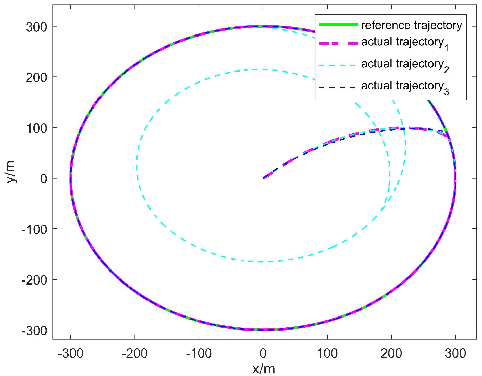
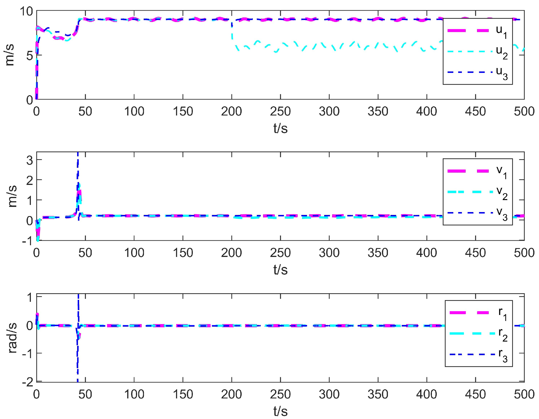
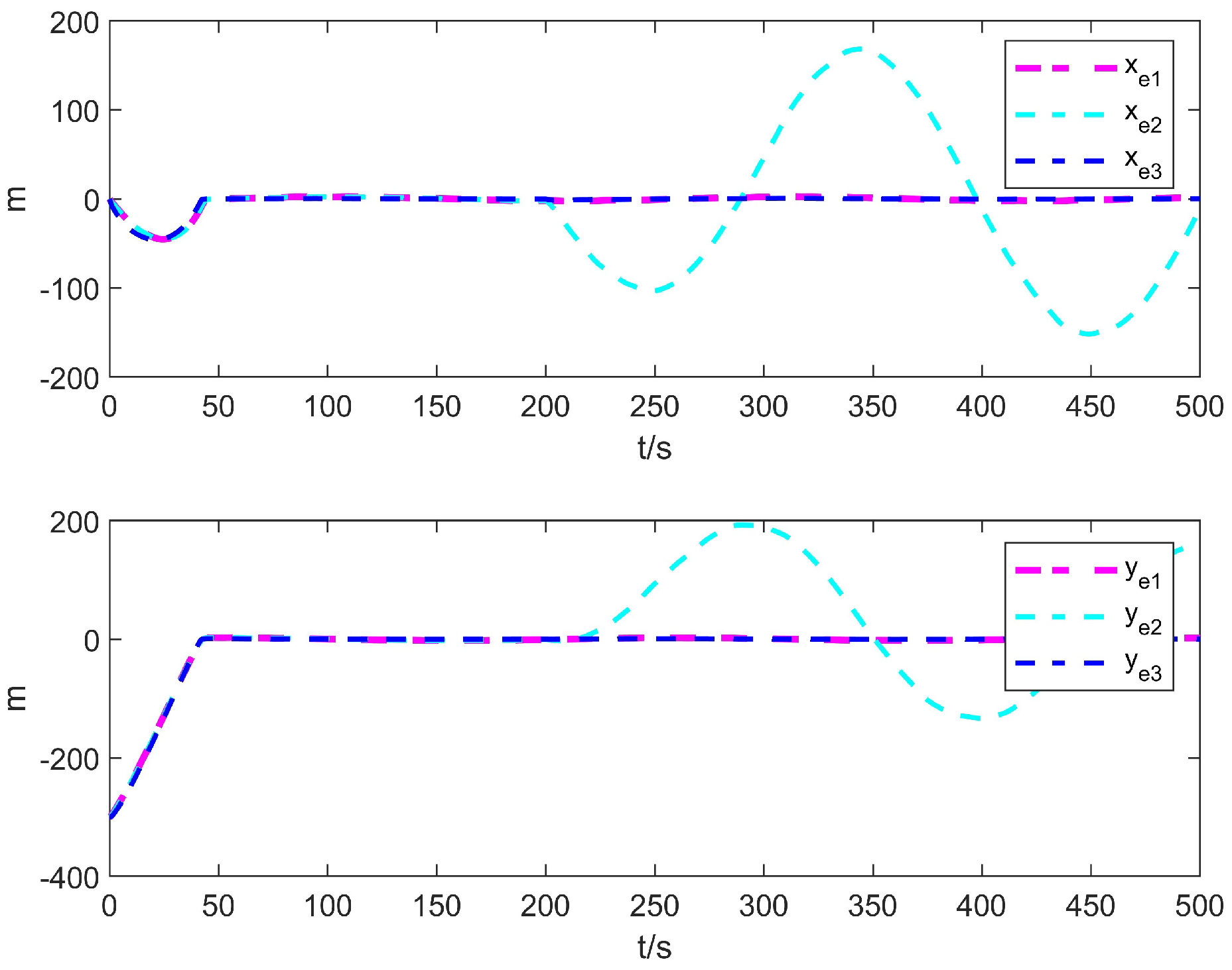
5. Simulation Results

To validate the control performance of the adaptive controller, numerical simulations were conducted in MATLAB/Simulink(R2024b) using the ship model described in Reference [25] as the test case. The parameters of the ship model are

$$m_{11}=1.20\times {10}^{5}kg,d_{11}=2.15\times {10}^{4}kg/s$$

$$m_{22}=1.779\times {10}^{5}kg,d_{22}=1.47\times {10}^{5}kg/s$$

$$m_{33}=6.36\times {10}^{7}kg,d_{33}=8.02\times {10}^{6}kg/s$$

The external environmental interference is

$$\left\{\begin{array}{c}{\tau }_{wu}={10}^5\left[sin\left(0.2t\right)+cos\left(0.5t\right)\right]\hfill \\ {\tau }_{wv}={10}^2\left[sin\left(0.1t\right)+cos\left(0.4t\right)\right]\hfill \\ {\tau }_{wr}={10}^6\left[sin\left(0.5t\right)+cos\left(0.3t\right)\right]\hfill \end{array}\right.$$

The unmodeled dynamics are as follows:

$$\left\{\begin{array}{c}{f}_u=0.2d_{11}{u}^2+0.1d_{11}{u}^3\hfill \\ f_v=0.2d_{22}{v}^2+0.1d_{22}{v}^3\hfill \\ f_r=0.2d_{33}{r}^2+0.1d_{33}{r}^3\hfill \end{array}\right.$$

The target trajectory is

$$x_d=300sin\left(0.03t\right)$$

$$y_d=300cos\left(0.03t\right)$$

The control parameters are shown in

Table 2. Control parameters.

Parameter	Value	Parameter	Value
c	9	k	5
${\alpha }_{u0}$	2	${\beta }_{u0}$	1
$q_{u0}$	5	$p_{u0}$	9
${\alpha }_{r0}$	1	${\beta }_{r0}$	1
$q_{r0}$	5	$p_{r0}$	9
${\alpha }_{r1}$	10	${\beta }_{r1}$	10
$q_{r1}$	1	$p_{r1}$	3
${\gamma }_{u1}$	$1\ast {10}^{-8}$	${\gamma }_{u2}$	$0.2$
$g_{u1}$	1	$g_{u2}$	$0.1$
${\gamma }_{r1}$	$1\ast {10}^{-8}$	${\gamma }_{r2}$	$0.2$
$g_{r1}$	1	$g_{r2}$	$0.1$

. The selection criteria for these parameters will be elaborated in subsequent sections.

The initial state is $x\left(0\right)=0$ m, $y\left(0\right)=0$ m, $\psi \left(0\right)=\pi /6rad$, $u\left(0\right)=0$ m/s, $v\left(0\right)=0$ m/s, $r\left(0\right)=0$ rad/s. The initial values of the parameter estimates are all set to 1. In RBF network design, the initial values of $\mathit{c}$ and $\mathit{b}$ should be configured within the effective mapping range of network inputs. Based on the actual range of network input $\mathit{z}={\left[u,v,r\right]}^T$, the Gaussian basis function parameters are determined as follows:

$$\left\{\begin{array}{c}{\mathbf{c}}_u=4\left[\begin{array}{ccccccccc}-6& -5.7& \cdots & -0.3& 0& 0.3& \cdots & 5.7& 6\\ -6& -5.7& \cdots & -0.3& 0& 0.3& \cdots & 5.7& 6\\ -6& -5.7& \cdots & -0.3& 0& 0.3& \cdots & 5.7& 6\end{array}\right]\hfill \\ {\mathbf{c}}_r=0.2\left[\begin{array}{ccccccccc}-1& -0.95& \cdots & -0.05& 0& 0.05& \cdots & 0.95& 1\\ -1& -0.95& \cdots & -0.05& 0& 0.05& \cdots & 0.95& 1\\ -1& -0.95& \cdots & -0.05& 0& 0.05& \cdots & 0.95& 1\end{array}\right]\hfill \\ b_{uj}=5,j=1,2,3\cdots 41\hfill \\ b_{rj}=2,j=1,2,3\cdots 41\hfill \end{array}\right.$$

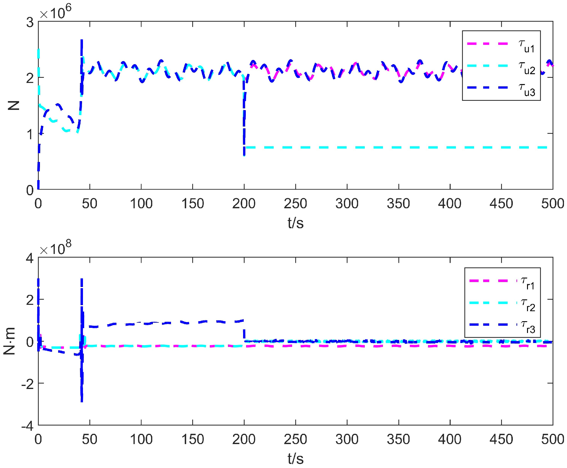
5.1. Control Performance Under Actuator Faults

When $t>200$ s, both actuators ${\tau }_u$ and ${\tau }_r$ experience faults with ${\sigma }_u=0.3$, ${\sigma }_r=0.1$, and ${\overline{\tau }}_u={\overline{\tau }}_r=0.8$. The related path-tracking results are shown in Figure 3, Figure 4, Figure 5, Figure 6 and Figure 7. (For clarity, subscript 1 denotes the case without faults, subscript 2 denotes the case with faults but without fault tolerance, and subscript 3 denotes the case with fault tolerance.) As shown in Figure 7, actuators ${\tau }_u$ and ${\tau }_r$ suffered severe failures at t = 200 s. From Figure 3, it can be observed that when actuator faults occurred, the non-fault-tolerant ship deviated from the desired trajectory, while the ship with our proposed fault-tolerant controller maintained accurate tracking of the reference path.

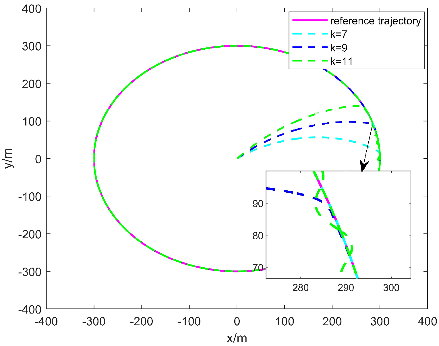
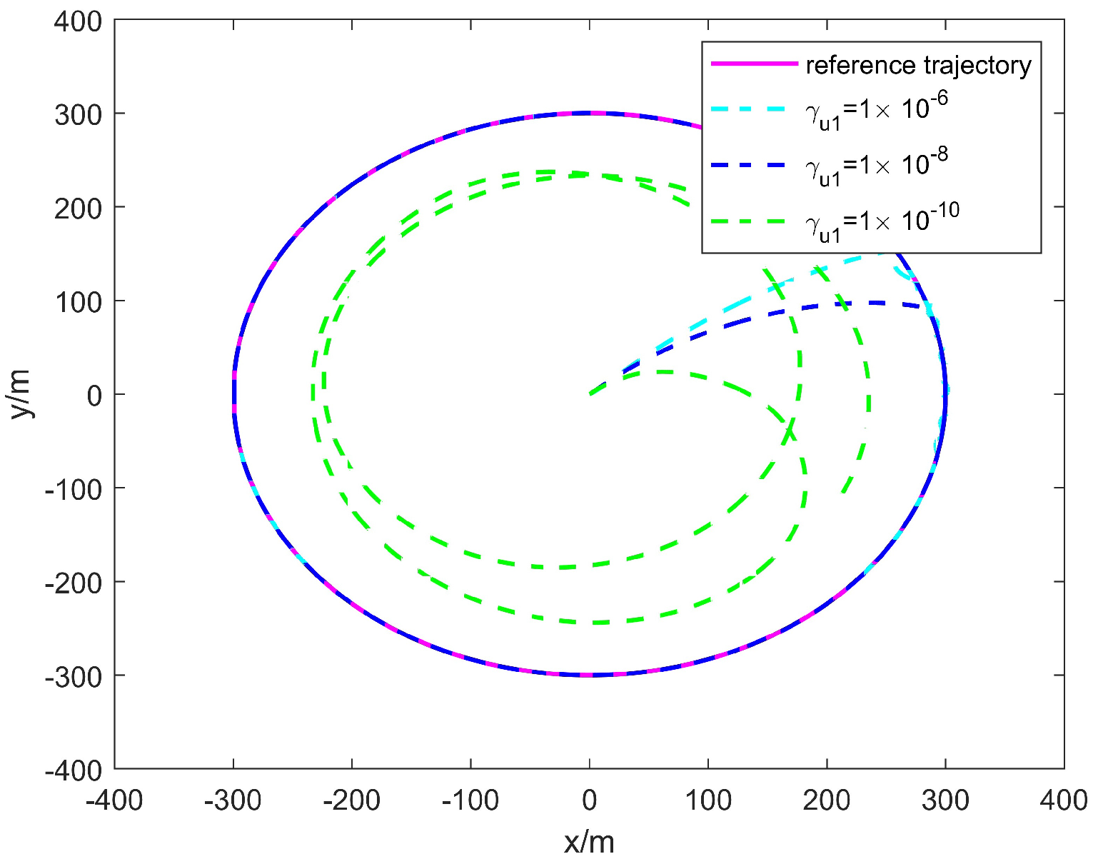
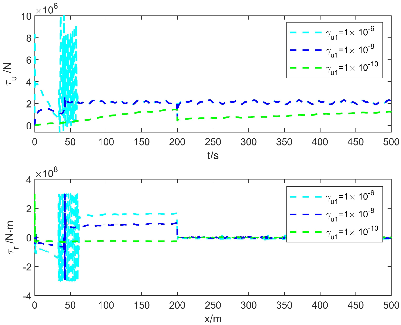
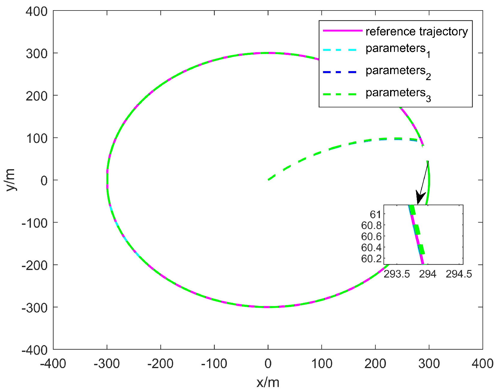
5.2. Impact of Parameters on Control Performance

Parameter selection significantly impacts the controller’s performance. The parameters k and ${\gamma }_{u1}$ are chosen as examples to demonstrate the influence of parameters on control performance.

As shown in Figure 8, the convergence rate is relatively slow when $k=7$, while with $k=11$, although fast convergence is achieved, the system only oscillates near the desired trajectory. Therefore, through comprehensive comparison, $k=9$ demonstrates the optimal convergence performance.

As shown in Figure 9, the system fails to track the reference path when ${\gamma }_{u1}=1\times {10}^{-10}$. While ${\gamma }_{u1}=1\times {10}^{-6}$ enables rapid path tracking, Figure 10 reveals severe actuator chattering occurs during the initial phase. Considering both convergence speed and actuator chattering, ${\gamma }_{u1}=1\times {10}^{-8}$ proves to be the most suitable parameter choice. The selection of other parameters also follows the same methodology.

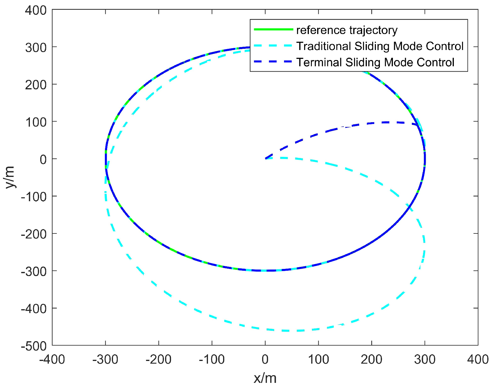
5.3. Comparison with Conventional Sliding Mode Control

A comparative analysis between the proposed fast terminal sliding mode and conventional sliding mode fault-tolerant control strategies reveals the following advantages of the proposed method:

Faster Convergence (Figure 11): The proposed approach demonstrates significantly improved convergence speed compared to traditional sliding mode control.

Enhanced stability under fault conditions (Figure 12): When faults occur, the proposed method exhibits substantially smaller oscillations than the conventional approach.

Reduced actuator chattering (Figure 13): The control signals generated by the proposed method show markedly less chattering behavior.

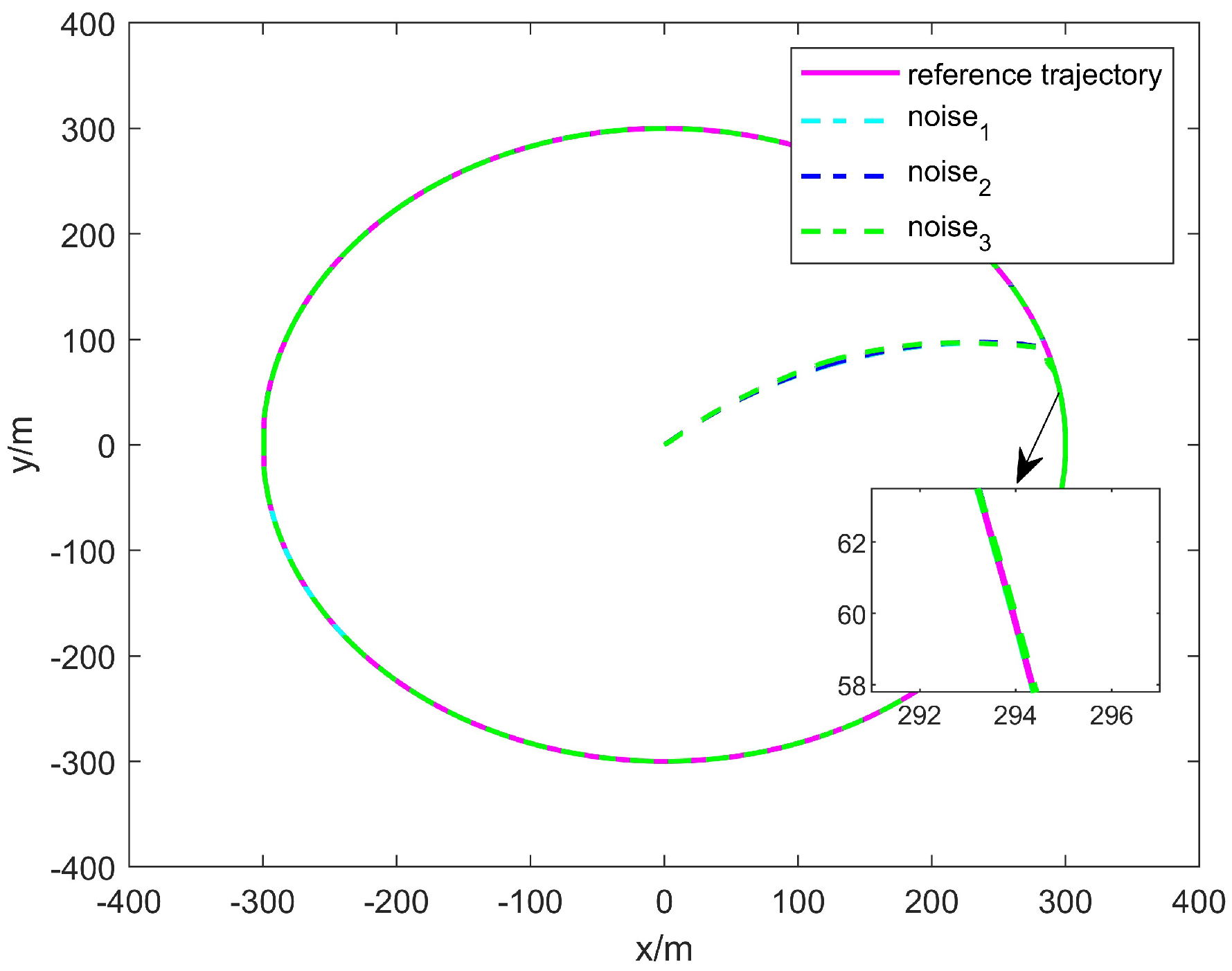
5.4. Robustness

This section presents the robustness test of the system. As shown in Figure 14 and Figure 15, the tracking performance remains virtually unaffected despite significant variations in external disturbances and system parameters.

The following explains the subscripts in the figures:

${\mathrm{noise}}_1$:

$$\left\{\begin{array}{c}{\tau }_{wu}={10}^3\left[sin\left(0.2t\right)+cos\left(0.5t\right)\right]\hfill \\ {\tau }_{wv}={10}^1\left[sin\left(0.1t\right)+cos\left(0.4t\right)\right]\hfill \\ {\tau }_{wr}={10}^5\left[sin\left(0.5t\right)+cos\left(0.3t\right)\right]\hfill \end{array}\right.$$

${\mathrm{noise}}_2$:

$$\left\{\begin{array}{c}{\tau }_{wu}={10}^5\left[sin\left(0.2t\right)+cos\left(0.5t\right)\right]\hfill \\ {\tau }_{wv}={10}^2\left[sin\left(0.1t\right)+cos\left(0.4t\right)\right]\hfill \\ {\tau }_{wr}={10}^6\left[sin\left(0.5t\right)+cos\left(0.3t\right)\right]\hfill \end{array}\right.$$

${\mathrm{noise}}_3$:

$$\left\{\begin{array}{c}{\tau }_{wu}={10}^6\left[sin\left(0.2t\right)+cos\left(0.5t\right)\right]\hfill \\ {\tau }_{wv}={10}^3\left[sin\left(0.1t\right)+cos\left(0.4t\right)\right]\hfill \\ {\tau }_{wr}={10}^7\left[sin\left(0.5t\right)+cos\left(0.3t\right)\right]\hfill \end{array}\right.$$

${\mathrm{parameters}}_1$:

$$\left\{\begin{array}{c}{m}_{11}=0.2\times {10}^5\mathrm{kg}\hfill \\ m_{22}=0.779\times {10}^5\mathrm{kg}\hfill \\ m_{33}=5.36\times {10}^7\mathrm{kg}\hfill \end{array}\right.$$

${\mathrm{parameters}}_2$:

$$\left\{\begin{array}{c}{m}_{11}=1.2\times {10}^5\mathrm{kg}\hfill \\ m_{22}=1.779\times {10}^5\mathrm{kg}\hfill \\ m_{33}=6.36\times {10}^7\mathrm{kg}\hfill \end{array}\right.$$

${\mathrm{parameters}}_3$:

$$\left\{\begin{array}{c}{m}_{11}=2.2\times {10}^5\mathrm{kg}\hfill \\ m_{22}=2.779\times {10}^5\mathrm{kg}\hfill \\ m_{33}=6.36\times {10}^7\mathrm{kg}\hfill \end{array}\right.$$

6. Conclusions

This paper investigates the adaptive fault-tolerant control problem for the USV with thruster failures while performing path tracking. Firstly, in the kinematic section, the desired speed of the USV is designed using the backstepping method based on the desired trajectory of the USV. Secondly, in the dynamic section, the fast terminal sliding mode control method is employed to enable the USV to track the desired speed, thereby achieving tracking of the desired trajectory. To address the composite disturbance composed of external disturbances, system unmodeled dynamics, actuator non-executed portions, and bias faults, an RBF neural network is utilized for approximation. Then, an adaptive law is designed to resolve the loss of effectiveness of the USV, and the stability and effectiveness of the designed controller are proven using Lyapunov functions. Finally, the feasibility of the proposed control method is verified through simulations.

References

- Li, J.; Zhang, G.; Jiang, C.; Zhang, W. A survey of maritime unmanned search system: Theory, applications and future directions. Ocean Eng. 2023, 285, 115359. [Google Scholar]
- Wang, Y.; Liu, W.; Liu, J.; Sun, C. Cooperative USV–UAV marine search and rescue with visual navigation and reinforcement learning-based control. ISA Trans. 2023, 137, 222–235. [Google Scholar] [PubMed]
- Jiang, X.; Xia, G. Event-Triggered Practical Formation Control of Leaderless Unmanned Surface Vehicles With Environmental Disturbances. IEEE Trans. Circuits Syst. II Express Briefs 2024, 71, 1326–1330. [Google Scholar]
- Lu, N.; Liu, H.; Wang, Y.; Yan, H. A new real-time path planning for USV based on dynamic artificial potential field in complex environments. Int. J. Robust Nonlinear Control. 2024. [Google Scholar] [CrossRef]
- Ning, J.; Wang, Y.; Liu, L.; Li, T. Disturbance observer based adaptive heading control for unmanned marine vehicles with event-triggered and input quantization. Int. J. Robust Nonlinear Control. 2024. [Google Scholar] [CrossRef]
- Fu, M.; Zhang, G.; Xu, Y.; Wang, L.; Dong, L. Discrete-time adaptive predictive sliding mode trajectory tracking control for dynamic positioning ship with input magnitude and rate saturations. Ocean Eng. 2023, 269, 113528. [Google Scholar]
- Zhou, B.; Huang, B.; Su, Y.; Zhu, C. Interleaved Periodic Event-Triggered Communications-Based Distributed Formation Control for Cooperative Unmanned Surface Vessels. IEEE Trans. Neural Netw. Learn. Syst. 2024, 36, 2382–2394. [Google Scholar]
- Peng, H.; Huang, B.; Jin, M.; Zhu, C.; Zhuang, J. Distributed finite-time bearing-based formation control for underactuated surface vessels with Levant differentiator. ISA Trans. 2024, 147, 239–251. [Google Scholar]
- Wang, Z.; Li, Y.; Ma, C.; Yan, X.; Jiang, D. Path-following optimal control of autonomous underwater vehicle based on deep reinforcement learning. Ocean Eng. 2023, 268, 113407. [Google Scholar]
- Xu, Z.; He, S.; Zhou, W.; Li, Y.; Xiang, J. Path Following Control With Sideslip Reduction for Underactuated Unmanned Surface Vehicles. IEEE Trans. Ind. Electron. 2024, 71, 11039–11047. [Google Scholar]
- Wang, S.; Sun, M.; Xu, Y.; Liu, J.; Sun, C. Predictor-Based Fixed-Time LOS Path Following Control of Underactuated USV With Unknown Disturbances. IEEE Trans. Intell. Veh. 2024, 8, 2088–2096. [Google Scholar] [CrossRef]
- Li, J.; Zhu, G.; Lu, J.; Chen, C. FTILOS-based self-triggered adaptive neural path following control for 4DOF underactuated unmanned surface vehicles. Ocean Eng. 2024, 295, 116947. [Google Scholar]
- Liang, H.; Li, H.; Xu, D. Nonlinear Model Predictive Trajectory Tracking Control of Underactuated Marine Vehicles: Theory and Experiment. IEEE Trans. Ind. Electron. 2021, 68, 4238–4248. [Google Scholar]
- Li, Y.; Feng, K.; Li, K. Finite-Time Fuzzy Adaptive Dynamic Event-Triggered Formation Tracking Control for USVs With Actuator Faults and Multiple Constraints. IEEE Trans. Ind. Inform. 2024, 4, 5285–5296. [Google Scholar] [CrossRef]
- Li, K.; Feng, K.; Li, Y. Fuzzy Adaptive Fault-Tolerant Formation Control for USVs With Intermittent Actuator Faults. IEEE Trans. Intell. Veh. 2024, 9, 4445–4455. [Google Scholar] [CrossRef]
- Wrat, G.; Ranjan, P.; Mishra, S.K.; Jose, J.T.; Das, J. Neural network-enhanced internal leakage analysis for efficient fault detection in heavy machinery hydraulic actuator cylinders. Proc. Inst. Mech. Eng. Part C J. Mech. Eng. Sci. 2025, 239, 1021–1031. [Google Scholar] [CrossRef]
- Hao, L.; Wu, Z.; Shen, C.; Cao, Y.; Wang, R. Tube-Based Model Predictive Control for Constrained Unmanned Marine Vehicles With Thruster Faults. IEEE Trans. Intell. Veh. 2024, 20, 4606–4615. [Google Scholar]
- Hao, L.; Zhang, Y.; Shen, C.; Xu, F. Fault-Tolerant Control for Unmanned Marine Vehicles via Quantized Integral Sliding Mode Output Feedback Technique. IEEE Trans. Intell. Transp. Syst. 2023, 24, 5014–5023. [Google Scholar] [CrossRef]
- Yang, X.; Hao, L.; Li, T.; Xiao, Y. Dynamic Positioning Control for Unmanned Marine Vehicles With Thruster Faults and Time Delay: A Lyapunov Matrix-Based Method. IEEE Trans. Syst. Man Cybern. Syst. 2024, 54, 4019–4030. [Google Scholar] [CrossRef]
- Wu, W.; Tong, S. Fixed-time formation fault tolerant control for unmanned surface vehicle systems with intermittent actuator faults. Ocean Eng. 2023, 281, 114813. [Google Scholar] [CrossRef]
- Sun, H.; Shi, J.; Hou, L. Dynamic Event-Triggered Output Feedback Fault-Tolerant Control for Dynamic Positioning of Unmanned Surface Vehicles With Multiple Estimators. IEEE Trans. Veh. Technol. 2024, 73, 3218–3229. [Google Scholar] [CrossRef]
- Liu, Z.; Wang, Y.; Han, Q. Adaptive fault-tolerant trajectory tracking control of twin-propeller non-rudder unmanned surface vehicles. Ocean Eng. 2023, 285, 115294. [Google Scholar] [CrossRef]
- Park, J.; Sandberg, I.W. Universal approximation using radial-basis-function networks. Neural Comput. 1991, 3, 246–257. [Google Scholar] [CrossRef] [PubMed]
- Xu, L.; Yao, B. Adaptive robust control of mechanical systems with non-linear dynamic friction compensation. Int. J. Control. 2008, 81, 167–176. [Google Scholar] [CrossRef]
- Do, K.D.; Jiang, Z.P.; Pan, J. Robust adaptive path following of underactuated ships. Automatica 2004, 6, 929–944. [Google Scholar]