A Novel Ship Fuel Sulfur Content Estimation Method Using Improved Gaussian Plume Model and Genetic Algorithms

Abstract

Maritime transportation plays a vital role in global economic development but is also a significant contributor to air pollution, especially through emissions of SO₂, NO_x, and CO₂. Identifying non-compliance with fuel sulfur content regulations is crucial for mitigating these environmental impacts, yet current methods face challenges, particularly in the absence of reliable CO₂ concentration data. This study proposes a novel inverse calculation framework to estimate ship fuel sulfur content without relying on CO₂ measurements. An improved Gaussian plume line source model was tailored to the dispersion characteristics of ship emissions, with influencing factors evaluated under varying wind field conditions. The emission source intensity inversion was formulated as an unconstrained multi-dimensional optimization problem, solved using genetic algorithms. By incorporating ship fuel consumption data derived from basic ship information, the sulfur content of ship fuels was effectively estimated. Experimental evaluations using 30 days of monitoring data revealed that the method successfully identified 2743 ships, with an overall detection rate of 82.72%. Among them, 131 ships were flagged as suspected of using high-sulfur fuel, and 111 were confirmed to be non-compliant via sampling and laboratory testing, achieving an accuracy of 84.73%. These results demonstrate that the proposed approach offers a reliable and efficient solution for real-time fuel sulfur content monitoring and enforcement under diverse atmospheric conditions, contributing to improved environmental management of maritime transport emissions.

1. Introduction

Maritime transportation is an important part of international trade, accounting for over 70% of trade worldwide. It also produces a large number of ship exhaust pollutions including carbon dioxide (CO₂), nitrogen oxides (NO_x), sulfur dioxide (SO₂), etc. According to the statistical analysis, ship emissions of CO₂, NO_x, and SO₂ account for 3%, 15%, and 4–9% of the global anthropogenic emissions, respectively [1,2,3]. These emissions have become major sources of air pollution in coastal and inland water regions [4,5,6]. To address air pollution caused by shipping, the International Maritime Organization (IMO) has established Sulfur Emission Control Areas, which set a maximum fuel sulfur content of 0.1% to be implemented globally by 2022 [7]. The Ministry of Transport and the Ministry of Ecology and Environment in China have also issued regulations such as “Implementation Plan for the Control Area of Air Pollutant Emissions from Ships” and “Yangtze River Economic Belt Ecological Environmental Protection Plan”. These regulations mandate that, from 1 January 2020, ships entering inland river emission control areas should use marine fuel with a sulfur content not exceeding 0.1% [8,9]. The challenge of real-time monitoring SO₂ and other pollutants emitted by ships and identifying fuel with excessive sulfur content effectively is a crucial and urgent task to maximize the impact of emission control areas [10,11].

Monitoring the concentration of ship pollutant emissions is fundamental to controlling excessive emissions. As one of the mainstream monitoring methods, aerial plume measurement is an indirect method for assessing ship emissions, based on the dispersion and dilution of exhaust plumes in the atmosphere. It calculates the emission source intensity by analyzing changes in the concentration of pollutants. Depending on the equipment type, aerial plume measurement can be classified into several types, including laser radar, spectral analyzers, sniffers, and portable multi-gas detectors [12,13,14]. Laser radar covers a wide monitoring area, but is expensive to install, maintain, and update, making it suitable for ports with concentrated berths. The sniffing technique involves quantifying ship emissions with portable devices mounted on various platforms, including aerial measurements conducted with aircraft [15,16,17]. This approach is efficient, and the findings are relatively dependable as it assesses the emission plume concentration directly [18]. Nevertheless, it depends on the apparent wind conditions and the location/distance of the measurement station [19,20]. Thus, the sniffing method is mainly suitable for ports where the prevailing wind direction is from sea to land. Portable multi-gas detectors offer quick and relatively reliable results, but their use requires boarding the ship, limiting the monitoring coverage. Spectral analysis techniques determine the type and concentration of gas plumes based on the Beer–Lambert principle and differential absorption spectroscopy [21,22]. The spectroscopy equipment can measure gas pollutant emissions from a long distance, which is generally loaded on land, ports, bridges, and other fixed locations. It has more advantages in terms of monitoring coverage, sensitivity, stability, and the ability to monitor a wide range of pollutants continuously [23,24].

After being emitted, gas pollutant emissions of ships immediately disperse and dilute in the air. This process makes it challenging to determine whether ship emissions exceed standards directly based on the concentration at the monitoring point, without quantitative inversion of emission source intensity [25]. Quantitative inversion of emission source intensity involves using measured pollutant concentration at the monitoring point to calculate the emission source intensity, defining whether emissions exceed the limits. This is a necessary component of effectively monitoring excessive ship emissions [26]. The random flow and dispersion characteristics of ship pollutant emissions make accurate monitoring difficult. Therefore, understanding the concentration distribution of pollutant emissions on a small scale under actual atmospheric conditions and establishing a small-scale dispersion model is crucial [27]. The Gaussian plume model, a commonly used continuous steady-state gas dispersion model, is simple in structure, accurate in simulation, and suitable for scenarios with prolonged emissions [28,29,30]. It can be used to analyze the dispersion process of ship pollutant emissions over a period, making it suitable for this study.

In addition, developing methods and technologies for identifying excessive sulfur content in marine fuel is essential for enforcing emission control area policies [31]. Among various methods for calculating fuel sulfur content of ships, the carbon balance method proposed by the IMO is commonly used. This method calculates the sulfur content based on the ratio of SO₂ and CO₂ concentration in ship pollutant emissions. The concentration of emissions recorded at the monitoring location does not correspond directly to the emissions released by ships, as there is a baseline level of this gas present even in the absence of ships. Consequently, the impact of background concentration is accounted for and eliminated during source intensity inversion using the carbon balance approach. This method requires the formation of distinct concentration peaks in the measurements, and the different monitoring principles of SO₂ and CO₂ may lead to the asynchronism of SO₂ and CO₂ concentration [32].

Although a variety of methods have been developed to analyze the dispersion process of ship pollutant emissions and calculate ship fuel sulfur content, the performance of these methods varies: (1) Existing methods for calculating fuel sulfur content primarily rely on the sulfur–carbon ratio and require CO₂ concentration data. There is a need for a method that uses only SO₂ emission source intensity data to calculate and identify the fuel sulfur content, when CO₂ monitoring concentration is unavailable or difficult to obtain. (2) Under actual atmospheric conditions, wind direction significantly influences the construction of ship exhaust dispersion models, especially when the wind direction does not align with the sailing direction. (3) While the Gaussian plume model is commonly employed, it is not fully suitable for certain environments, particularly in marine settings where meteorological conditions are complex. Therefore, several adjustments are necessary to the standard Gaussian plume model regarding effective wind speed, dispersion coefficients, and emission source height.

With these considerations, the focus of this study is to obtain the ship SO₂ emission data using spectroscopy remote sensing, and develop an improved Gaussian plume line source model under changing wind fields. Drawing from an analysis of earlier research, this study enhances the standard Gaussian plume model by refining four key elements: effective wind speed, the height of the emission source, dispersion coefficients, and the angle between the wind direction and the direction of travel. An intelligent optimization algorithm is explored to conduct the quantitative inversion of source intensity for ship emissions. Using genetic algorithms, the emission source intensity inversion problem is transformed into an unconstrained multi-dimensional extremum problem. In addition, a calculation method for ship fuel consumption is developed using the basic information of ships, and a method for calculating the fuel sulfur content without relying on CO₂ concentration is proposed. The suggested method offers an effective and precise means of monitoring the measurement of ship fuel sulfur content.

2. Method

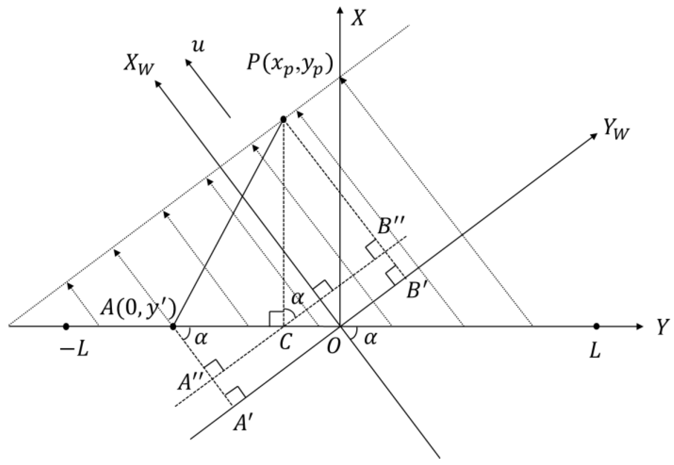
2.1. Gaussian Plume Line Source Model

The Gaussian plume model is a commonly used continuous steady-state gas dispersion model, which is suitable for scenarios involving long-term emissions from a source. This model operates under several fundamental assumptions. It assumes that the emission source is continuous and steady-state, meaning that pollutants are emitted at a constant rate over time. The dispersion of pollutants follows a Gaussian distribution in both horizontal and vertical directions, with concentrations decreasing symmetrically as the distance from the source increases. Atmospheric conditions, including wind speed, wind direction, and stability, are considered homogeneous and constant across the area of interest. The model also accounts for the reflection of pollutants from the ground or water surface, with a reflection ratio applied to estimate the proportion of pollutants returning to the atmosphere. Additionally, it assumes that pollutants remain chemically inert during dispersion and that the effective emission source height is determined by the sum of the physical chimney height and the plume rise. These assumptions provide a simplified yet robust framework for modeling pollutant dispersion in the atmosphere.

This model features a straightforward structure and provides accurate simulations, founded on the principles of normal distribution and turbulent diffusion statistics. The concentration of ship pollutant emissions at a given point $(x,y,z)$, represented as $c(x,y,z)$, is determined by both the physical source and an associated virtual source. Under optimal conditions, gas emissions are ultimately observed upon reaching the surface. However, this reflection occurs off the water surface rather than land. As the gas emissions spread over the water, they are reflected back into the atmosphere. The extent of reflected dispersed matter is influenced by the diameter of the particulate matter: bigger particles experience greater losses due to gravitational settling. Based on the Gaussian plume model, the concentration from the actual source, with a vertical height difference of z − H, can be expressed as follows:

$$c_s={\displaystyle \frac{Q}{2\pi u{\sigma }_y{\sigma }_z}}{e}^{{\displaystyle \frac{-y^2}{2{{\sigma }_y}^2}}}·e^{{\displaystyle \frac{-{\left(z-H\right)}^2}{2{{\sigma }_z}^2}}}$$

(1)

where $c_s$ is the dispersion concentration from source intensity (kg/m³); Q represents the source intensity (discharge rate) of emissions (kg/s); ${\sigma }_y$ and ${\sigma }_z$ denote the dispersion coefficients in the y (longitude) and z (vertical) directions, respectively; H is the effective height of the emission source from the ground (m); $u$ represents the effective wind speed (m/s).

The virtual source’s dispersion effect, with a vertical height difference of $z+H$, can be expressed as follows:

$$c_s^{\prime }={\displaystyle \frac{R·Q}{2\pi u{\sigma }_y{\sigma }_z}}{e}^{{\displaystyle \frac{-y^2}{2{{\sigma }_y}^2}}}·e^{{\displaystyle \frac{-{\left(z+H\right)}^2}{2{{\sigma }_z}^2}}}$$

(2)

The concentration of virtual source intensity diminishes as a result of losses and other factors during the gas reflection process. If we denote the reflection ratio as $(R\in \left[\mathrm{0,1}\right])$, the overall concentration arising from both the actual and virtual sources can be expressed as follows:

$$c=c_s+c_s^{\prime }={\displaystyle \frac{Q}{2\pi u{\sigma }_y{\sigma }_z}}{e}^{-{\displaystyle \frac{y^2}{2{{\sigma }_y}^2}}}\left[e^{-{\displaystyle \frac{{\left(z-H\right)}^2}{2{{\sigma }_z}^2}}}+R·e^{-{\displaystyle \frac{{\left(z+H\right)}^2}{2{{\sigma }_z}^2}}}\right]$$

(3)

When a ship travels along the waterway, it can be regarded as a continuous emission source. The emission sources along the route create discontinuous concentration fields on either side, which can be modeled as a finite-length line source. Under actual sailing conditions, the wind direction significantly influences the construction of ship exhaust dispersion models, especially when the wind direction does not align with the sailing direction. As illustrated in Figure 1, when the emission source (i.e., the ship) emits continuously and moves horizontally, the concentration of pollutant emissions from the line source is uniform across the crosswind direction. The moving emission source can be divided into N equal segments along the horizontal length, integrating the concentration at all points along the finite length to determine the concentration at any downwind point.

In Figure 1, $P(x_p,y_p)$ represents the monitoring point coordinates; $A(0,y^{\prime })$ represents the ship position coordinates; and $\alpha$ is the angle between the wind direction and line source (i.e., sailing direction). Ship emission diffusion consists of two components: one moving in the sailing direction and the other moving in the wind direction, influenced by wind speed. The combined vector of the wind direction, wind speed, the sailing direction, and sailing speed represents the actual dispersion direction of the ship pollutant emissions. Using the wind direction as the $X_W$ axis and the direction perpendicular to the wind as the $Y_W$ axis, lines are drawn through points A and P perpendicular to the $Y_W$ axis, intersecting at points $A^{\prime }$ and $B^{\prime }$, respectively. The projected distance on the $Y_W$ axis between the ship position and the monitoring point is $A^{\prime }{B}^{\prime }$. Drawing a line from point P perpendicular to the Y axis intersecting at point C, and a parallel line from point C to $A^{\prime }{B}^{\prime }$, intersecting $A{A}^{\prime }$ at point $A^{″}$ and ${PB}^{\prime }$ at point $B^{″}$, $\angle {PCB}^{″}=\angle {CAA}^{″}=\alpha$, then:

$$A^{\prime }{B}^{\prime }=A^{″}{B}^{″}=AC·\sin \alpha +PC·\cos \alpha =\left(y_p-y^{\prime }\right)\sin \alpha +x_p\cos \alpha$$

(4)

To estimate the concentration caused by a finite-length line source, the edge effect caused by the line source’s endpoints should be considered. As the distance between the receiving point and the line source increases, the edge effect becomes more pronounced at greater lateral distances. For a finite-length crosswind line source, if the line source extends from −L to L, the finite-length line source dispersion model integrates the variable $y^{\prime }$ from −L to L. The integral formula for the dispersion of ship pollutant emissions is

$$C\left(x_p,y_p,z,\alpha \right)={\displaystyle \frac{Q}{2\pi u{\sigma }_y{\sigma }_z}}{\int }_{-L}^L{e}^{-{\displaystyle \frac{{\left[\left(y_p-y^{\prime }\right)\sin \alpha +x_p\cos \alpha \right]}^2}{2{{\sigma }_y}^2}}}\left[e^{-{\displaystyle \frac{{\left(z-H\right)}^2}{2{{\sigma }_z}^2}}}+R·e^{-{\displaystyle \frac{{\left(z+H\right)}^2}{2{{\sigma }_z}^2}}}\right]d{y}^{\prime }$$

(5)

where R is the reflection ratio. The emitted SO₂ features small particle sizes, making its impact on reflection negligible. Nevertheless, SO₂ is soluble in water and undergoes a chemical reaction. Based on pertinent studies, the reflection ratio R can be established at 0.9 [33].

(1)

Emission Source Height Modification

$$H=H^{\prime }+\Delta h$$

(6)

where $H$ is the effective emission source height; $H^{\prime }$ is the geometric height of the ship chimney (m); $\Delta h$ represents the plume lifting height (m). The height at which the plume rises is influenced by various factors, including buoyancy characteristics, the downwind distance from the source, the speed of the vessel, the temperature of the emission source, ambient temperature, and the diameter of the chimney. These factors can be difficult to measure accurately for different vessels. Therefore, this study employs an empirical approach: the recommended $\Delta h$ is 15 m when $H^{\prime }$ is over 50 m; $\Delta h$ is 8 m when $H^{\prime }$ is between 30 m and 50 m; $\Delta h$ is 5 m when $H^{\prime }$ is under 30 m [34]. In real sailing conditions, when the chimney height of the ship is relatively low, the plume lifting height can be estimated using linear interpolation [32].

(2)

Wind Speed Modification

There is a discrepancy between the effective wind speed and ground-level wind speed, and wind speed varies with different heights. Thus, wind speed modification is necessary:

$$u=u_g{\left({\displaystyle \frac{H}{H_g}}\right)}^m$$

(7)

where $u$ demotes the effective wind speed; $u_g$ is the ground-level wind speed measured by a meteorological instrument (m/s); $H_g$ is the height of the meteorological instrument position (m); m is the power law constant determined by the atmospheric stability level [26]. Atmospheric stability is a measure of the vertical consistency of the atmosphere, reflecting the degree of turbulence present. A higher level of stability reduces the potential for air to spread. Atmospheric stability depends on several factors such as observation time, solar hour angle, solar dip angle, solar altitude angle, cloud cover, solar incidence class, and wind speed. Initially, the solar hour angle is computed using local longitude and the timing of observation. Following this, the solar altitude angle is calculated based on the solar hour angle, solar dip angle, and local latitude. The solar incidence classification is established by analyzing the solar altitude angle along with cloud cover. Finally, atmospheric stability is ranked from grade A to F, where A indicates a high degree of instability, B signifies instability, C shows mild instability, D is neutral, E implies mild stability, and F denotes full stability. The method for determining atmospheric stability can be found in the relevant literature [26].

(3)

Dispersion Coefficient Modification

Dispersion coefficients in atmospheric dispersion models are functions of atmospheric stability and downwind distance. These coefficients can be determined by empirical methods and are considered as constants. Traditional empirical methods can characterize gas dispersion over long distances, but they lack resolution and accuracy for small-scale dispersion, such as ship pollutant emissions. Thus, the traditional empirical dispersion coefficient equation is modified by introducing different directional dispersion coefficients:

$$\left\{\begin{array}{c}{\sigma }_y={\displaystyle \frac{{\gamma }_{1,y}·x}{{\left(1+{\gamma }_{2,y}·x\right)}^{{\alpha }_y}}}\\ {\sigma }_z={\displaystyle \frac{{\gamma }_{1,z}·x}{{\left(1+{\gamma }_{2,z}·x\right)}^{{\alpha }_z}}}\end{array}\right.$$

(8)

where x represents the downwind distance from the emission source (m); ${\gamma }_{1,y}$ and ${\gamma }_{1,z}$ are the horizontal dispersion coefficients; ${\gamma }_{2,y}$ and ${\gamma }_{2,z}$ are the vertical dispersion coefficients; ${\alpha }_y$ and ${\alpha }_z$ are the dispersion indices (m). Regarding the dispersion of emissions from ships, the marine environment offers a vast open space. Unlike in urban settings, there are no tall buildings that could obstruct the movement of pollutants. As a result, the diffusion characteristics are more akin to those found in rural settings, leading to the selection of a diffusion coefficient equation that is appropriate for rural conditions. The values can be obtained from the Briggs dispersion coefficient equations [32,35], as shown in

Table 1. Briggs diffusion coefficient.

Atmospheric Stability		${\mathit{\gamma }}_{\mathbf{1}\mathbf{,}\mathit{y}}$	${\mathit{\gamma }}_{\mathbf{2}\mathbf{,}\mathit{y}}$	${\mathit{\alpha }}_{\mathit{y}}$	${\mathit{\gamma }}_{\mathbf{1}\mathbf{,}\mathit{z}}$	${\mathit{\gamma }}_{\mathbf{2}\mathbf{,}\mathit{z}}$	${\mathit{\alpha }}_{\mathit{z}}$
Rural condition	A	0.22	0.0001	0.5	0.20	0	1.0
	B	0.16	0.0001	0.5	0.12	0	1.0
	C	0.11	0.0001	0.5	0.08	0.0002	0.5
	D	0.08	0.0001	0.5	0.06	0.0015	0.5
	E	0.06	0.0001	0.5	0.03	0.0003	1.0
	F	0.04	0.0001	0.5	0.02	0.0003	1.0

. As the downwind distance increases, the dispersion coefficients increase gradually. In general, for the same downwind distance, the dispersion coefficients decrease with increasing atmospheric stability levels.

2.2. SO₂ Quantitative Inversion of Source Intensity

Inversion algorithms are widely used in environmental studies to estimate unknown parameters, such as emission source intensity, based on observed data. These algorithms transform the problem into an optimization task, where the goal is to minimize the difference between observed and modeled data. In this study, a genetic algorithm is employed as the inversion method to estimate the emission source intensity of ship pollutants.

The emission source intensity Q can be calculated using the monitoring concentration c from the dispersion model described above. Traditional methods for source intensity inversion based on probabilistic statistical models require prior probability distribution information and extensive statistical data. In contrast, optimization model methods establish quantitative relationships between ship emission sources, pollutant dispersion, and monitoring values. By minimizing the errors between monitoring and calculating values, the source intensity inversion process is transformed into an optimization problem, which can be solved using intelligent optimization algorithms to find the solution that minimizes the target value [36,37]. The target function $f\left(Q\right)$ is the sum of the squared errors between the monitoring concentration $C_m^i$ and the calculating concentration $C_c^i$ at each monitoring point:

$$\underset{Q}{\min }f\left(Q\right)={\sum }_{i=1}^n{\left(C_m^i-C_c^i\right)}^2$$

(9)

This study aims to solve the complex optimization problem of ship fuel sulfur content inversion, which involves multiple nonlinear variables such as emission source strength, wind speed, and diffusion coefficients. Traditional methods often get stuck in local optima and struggle to address these complex relationships and uncertainties. The genetic algorithm, with its global search capability and adaptability to complex nonlinear problems, effectively solves these issues. By simulating the process of natural evolution, the algorithm gradually optimizes the solution and avoids local optima, while demonstrating strong robustness in uncertain environments. Moreover, the genetic algorithm does not rely on extensive prior information, making it particularly suitable for the multi-dimensional optimization needs of ship fuel sulfur content inversion.

Using genetic algorithms to solve this unconstrained optimization problem, the parameters are encoded as chromosomes, and the population evolves towards the optimal solution through iterative selection, crossover, and mutation operations. The steps include: (1) encoding the solution space data into chromosome-like string structures; (2) generating an initial population by randomly creating N initial strings containing source intensity information, which serves as the starting point for evolution; (3) substituting the population’s individuals into the target function to calculate and rank the chromosome values; (4) selecting the best individuals from the current population based on the principle of survival of the fittest; (5) randomly crossing different individuals to produce new individuals and populations; (6) introducing mutations in a small portion of the population to escape local optimal with a given probability; (7) ending the iteration by setting conditions such as the maximum number of iterations and iteration time.

2.3. Fuel Sulfur Content Estimation

The fuel sulfur content can be represented as the ratio of the SO₂ emission rate (i.e., emission source intensity Q) to the ship fuel consumption rate M. Given the molecular mass ratio of SO₂ to sulfur S is 64:32 = 2:1, the fuel sulfur content can be expressed as follows:

$$S={\displaystyle \frac{Q}{2M}}$$

(10)

where S represents the fuel sulfur content (%); M represents the ship fuel consumption rate (kg/s), which can be determined using the ship main engine basic fuel consumption coefficient, main engine power, main engine fuel consumption rate, auxiliary engine power, and auxiliary engine fuel consumption rate:

$$M=p\ast A_1+A_2$$

(11)

$$A_1=a_1\ast b_1$$

(12)

$$A_2=a_2\ast b_2$$

(13)

where p is the main engine basic fuel consumption coefficient, with typical values of 0.7 for cargo-oil, cargo-gas, and cargo-chemical tankers, 0.8–0.9 for cargo-bulk carrier and general cargo, 0.5–0.7 for harbor ship-tugs, and 1.0 for passenger ships [38]. $A_1$ and $A_2$ represent the main and auxiliary engine fuel consumption ($\mathrm{k}\mathrm{g}/\mathrm{h}$); $a_1$ and $a_2$ represent the main and auxiliary engine power (kw); and $b_1$ and $b_2$ represent the main and auxiliary engine fuel consumption rates ($\mathrm{k}\mathrm{g}/\mathrm{k}\mathrm{w}·\mathrm{h}$). The main engine fuel consumption rate typically ranges from 0.165 to 0.178 $\mathrm{k}\mathrm{g}/\mathrm{k}\mathrm{w}·\mathrm{h}$, and the auxiliary engine fuel consumption rate ranges from 0.019 to 0.025 $\mathrm{k}\mathrm{g}/\mathrm{k}\mathrm{w}·\mathrm{h}$ in the setup of the experiment [39]. However, the above fuel consumption rates are only likely in a certain load range (i.e., 25–75%) and could be significantly higher outside this range. Therefore, the effective variation in fuel consumption rates is in fact much larger in the setup of the experiment (0.150–0.300 $\mathrm{k}\mathrm{g}/\mathrm{k}\mathrm{w}·\mathrm{h}$ for main engine and 0.015 to 0.030 $\mathrm{k}\mathrm{g}/\mathrm{k}\mathrm{w}·\mathrm{h}$ for auxiliary engine is a more correct range in real operations). Several formulas are used to calculate main and auxiliary engine power of ships, such as Ship Traffic Emission Assessment Model (STEAM) and improved STEAM2 [40,41]. Many parameters are needed for these methods, but obtaining them for different ships can be challenging. As a result, this study utilizes a method that combines data from various sources with regression fitting to obtain the ship main and auxiliary engine power, based on the ship static information from the automatic identification system (AIS) and the Lloyd’s Register database [42], as shown in

Table 2. Regression function between gross tonnage and main, auxiliary engine power.

Ship Categories	Sample Size	Regression Function Between Gross Tonnage (GT) and Main Engine Power	Auxiliary to Main Engine Power Ratios	${\mathit{R}}^{\mathbf{2}}$
Cargo-Bulk carrier	28,320	$a_1=10.051{ \times GT}^{0.652}$	$a_2=0.253a_1$	0.947
Cargo-Oil tanker	34,026	$a_1=4.901{ \times GT}^{0.729}$	$a_2=0.342a_1$	0.935
Cargo-Container	73,967	$a_1=3.191{ \times GT}^{0.844}$	$a_2=0.223a_1$	0.938
Cargo-General cargo	13,809	$a_1=2.104{ \times GT}^{0.838}$	$a_2=0.238a_1$	0.802
Harbor ship-Tugs	40,346	$a_1=74.340{ \times GT}^{0.563}$	$a_2=0.126a_1$	0.746
Cargo-Chemical tanker	28,147	$a_1=2.622{ \times GT}^{0.817}$	$a_2=0.363a_1$	0.929
Cargo-Gas tanker	39,165	$a_1=24.627{ \times GT}^{0.584}$	$a_2=0.337a_1$	0.933
Cargo-Ro-Ro carrier	67,838	$a_1=69.865{ \times GT}^{0.558}$	$a_2=0.277a_1$	0.731
Passenger	80,998	$a_1=26.769{ \times GT}^{0.458}$	$a_2=0.079a_1$	0.746

.

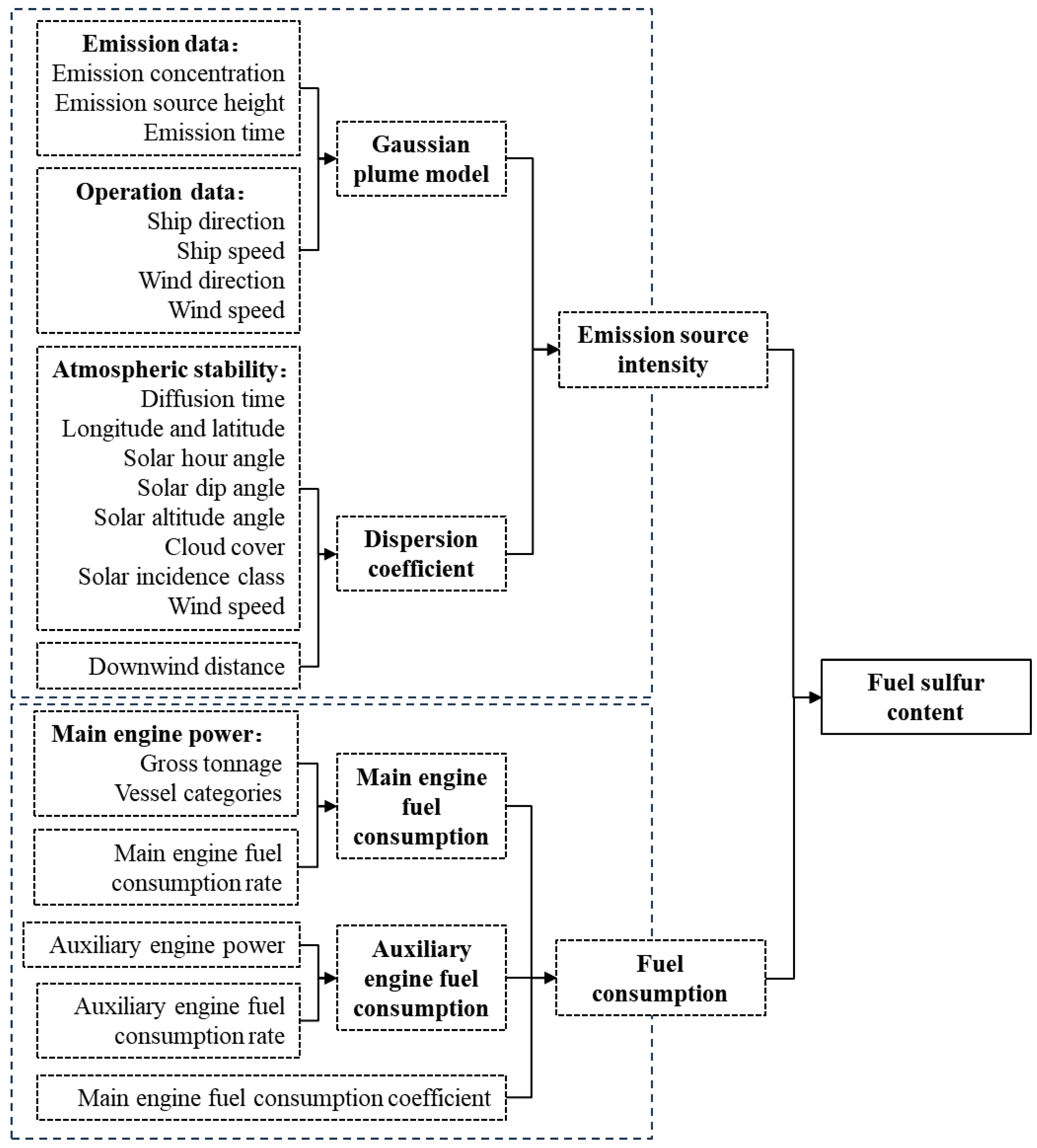
2.4. Overview of the Methodology

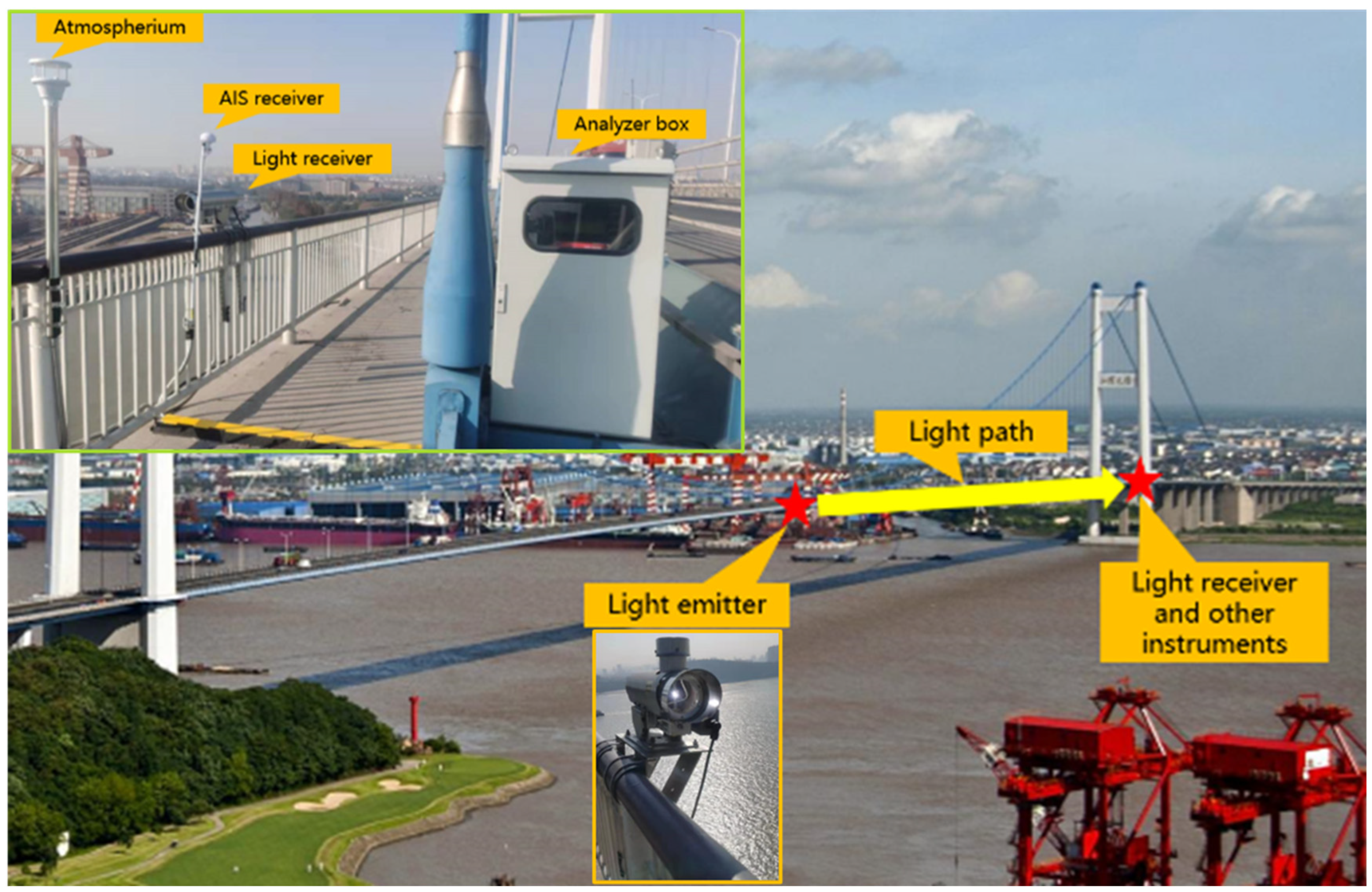
Figure 2 illustrates the overall methodological framework employed in this study, which consists of three key steps. First, meteorological and air quality monitoring data from ship plumes are utilized, and the Gaussian dispersion model is applied to calculate the pollutant concentration distribution (SO₂ concentration). Second, using an inversion algorithm and the monitoring data, the emission source intensity of the ships is estimated. Third, based on the computed emission intensity and ship activity data, the fuel consumption (from main and auxiliary engines) is determined. Finally, by comparing the estimated fuel consumption with reported data, the sulfur content in the fuel is derived. This methodology integrates monitoring, modeling, and optimization to provide a comprehensive solution for assessing and monitoring ship emissions.

3. Data Collection

In earlier engineering applications of the research team, monitoring equipment equipped with a spectral analysis remote sensing system was installed at the Nanjing Dashengguan Yangtze River Bridge in 2021, connecting the Pukou District with urban areas of Nanjing, China. These installations can be used for the real-time concentration data collection and monitoring of the ship pollutant emissions. The Nanjing Dashengguan Yangtze River Bridge has a clear width of 650 m, with the transmitter of monitoring equipment placed on the deck of the bridge over the upstream channel and the receiver located on the maintenance platform of the north tower. The total light path is approximately 350 m, enabling monitoring coverage of upstream ships. The dedicated 4G network signal on the bridge is robust, supporting data transmission for the spectral equipment. Figure 3 illustrates the monitoring equipment, which comprises three components: the analyzer box, light emitter, and light receiver. The light source and detector create an unobstructed illumination pathway using a xenon lamp in the transmitter, directing light towards the detector. The analysis unit quantifies the substances by evaluating the reduction they cause in the detected spectrum.

Pollutant emissions from motor vehicles on the bridge do not affect the monitoring of ship exhaust for several reasons: (1) the sulfur content in vehicle fuel is considerably lower than in marine fuel for SO₂; (2) vehicle exhaust plumes initially rise due to thermal effects before gradually diluting, leading to limited lateral diffusion; (3) while a large number of vehicles can influence SO₂ concentrations, this impact is generally stable over short periods. As motor vehicles continuously release pollutants while passing through the monitoring area, the resulting SO₂ concentration fluctuations are considered part of the background concentration in this study.

The data collection includes measured SO₂ emission concentration, ship dynamic information (latitude and longitude, ship speed, ship direction, distance from the monitoring point, etc.), ship static information (MMSI number, ship length, type, number, gross tonnage, etc.), and meteorological data (wind speed, wind direction, etc.). Wind speed and wind direction data can be obtained using an anemometer, which provides real-time measurements and continuous tracking of wind changes. The anemometer can measure wind speeds up to 60 $\mathrm{m}/\mathrm{s}$ and provide full 360-degree coverage for wind direction, with $\pm 3$ degrees for accuracy and resolution.

4. Results and Analysis

To illustrate and validate the effectiveness of the proposed method for calculating ship fuel sulfur content, three cases were presented in this section: (1) Selecting one ship detected with sulfur content exceeding the standard (the fuel sulfur content should be less than 0.1%, exceeding 0.1% is considered non-compliant) to introduce the analysis process of calculating fuel sulfur content without relying on CO₂ concentration. The fuel of this suspected ship was sampled by the maritime authorities using portable analytical instruments to verify fuel sulfur content estimation accuracy. (2) Using 97 exempted ships information provided by the maritime authorities to validate the effectiveness of the quantitative inversion of source intensity and fuel sulfur content estimation method. (3) Randomly selecting the operation data for 30 consecutive days to show the actual monitoring effect and evaluate the stability and practicality of this method.

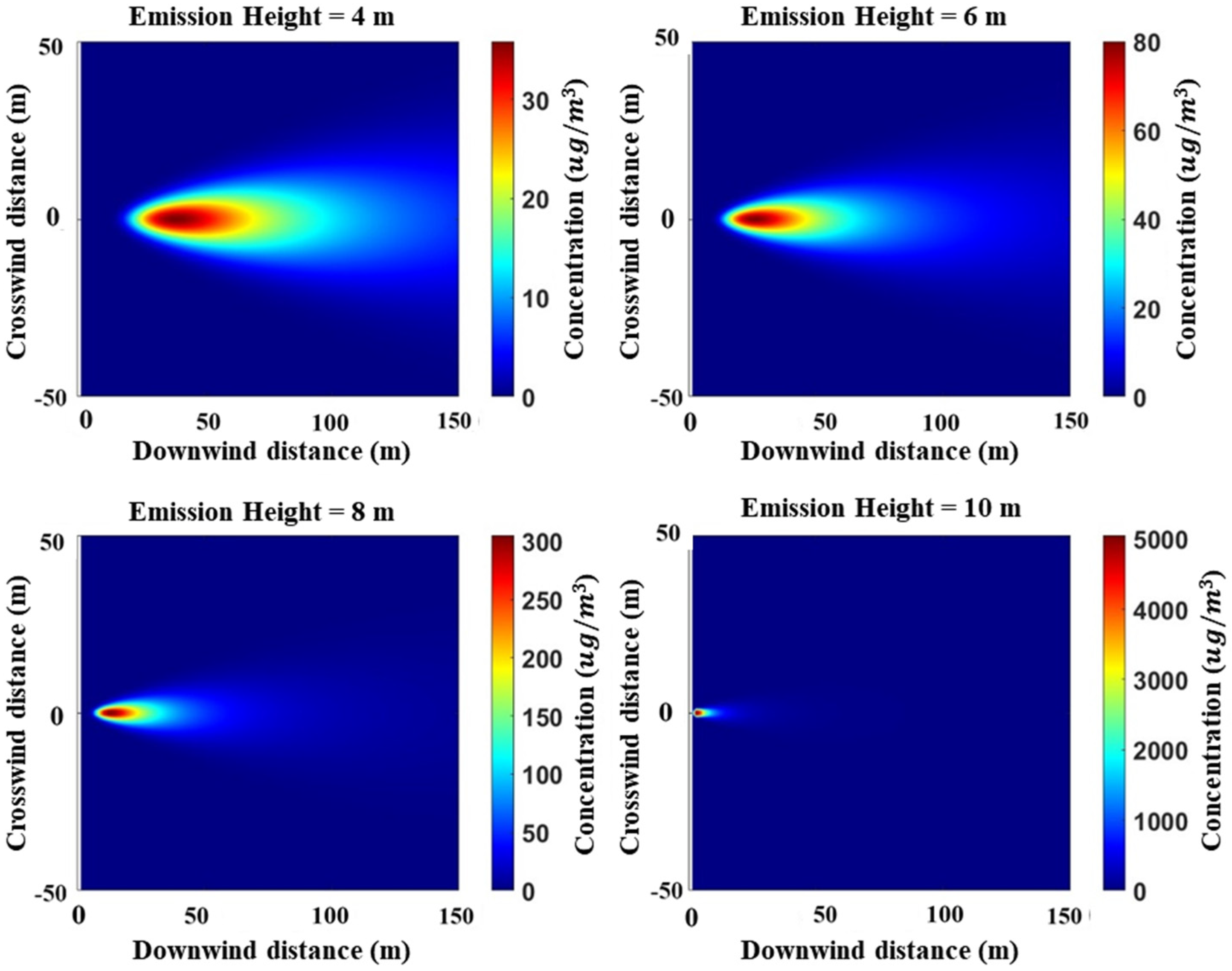
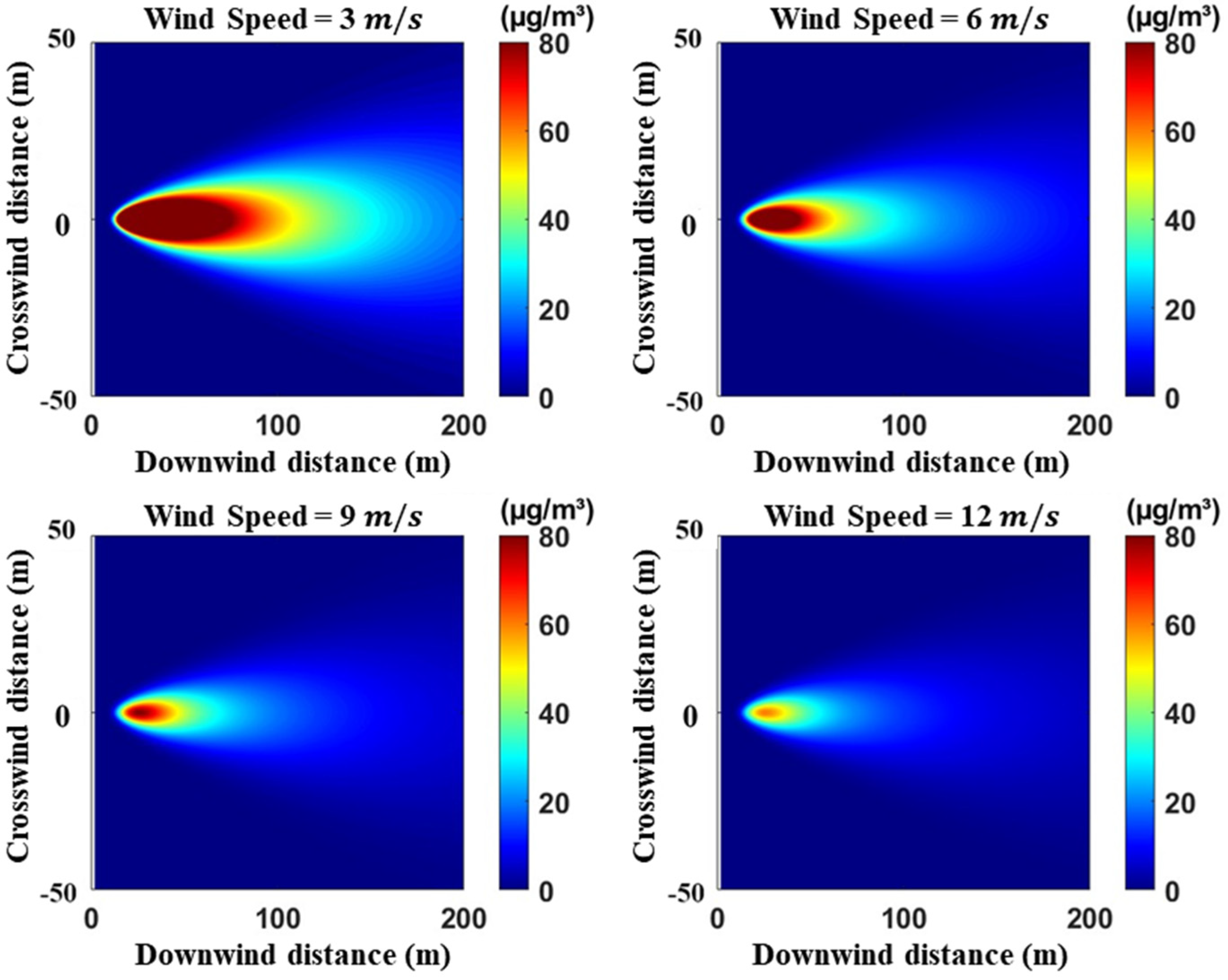
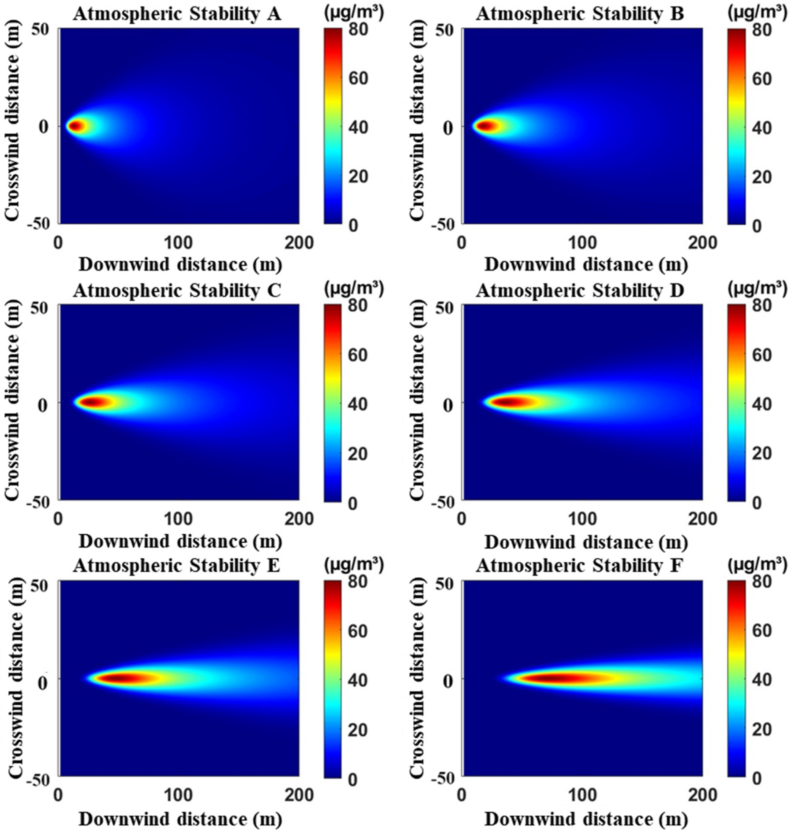
4.1. Simulation Results of Ship Exhaust Gas Diffusion

To analyze the dispersion characteristics of ship exhaust emissions under different conditions, this study conducted comparative dispersion simulation experiments focusing on emission source height, wind speed, and atmospheric stability. To ensure the scientific rigor and consistency of the simulation results, the following default parameters were adopted: the emission source strength was set to 0.1 $\mathrm{g}/\mathrm{s}$, representing a typical emission rate for ship exhaust; the initial wind speed was set to 9 $\mathrm{m}/\mathrm{s}$, and the wind direction was fixed at 270°. The emission source height was set to 6 m, corresponding to the average height of ship chimneys, while the monitoring height was set to 10 m to simulate the typical position of monitoring equipment. Additionally, the ambient temperature was assumed to be 15 °C, representing standard atmospheric conditions, and the atmospheric stability class was set to Category C, indicating slightly unstable conditions conducive to moderate dispersion. These parameter settings were chosen to simulate realistic scenarios and evaluate the model’s performance under typical maritime environmental conditions. By systematically adjusting individual parameters, these simulations comprehensively reveal the influence of factors such as emission source height, wind speed, and atmospheric stability on the dispersion characteristics and pollutant concentration distributions of ship emissions.

Figure 4 presents the results of exhaust gas dispersion at different emission heights under a monitoring height of 10 m, including emission heights of 4 m, 6 m, 8 m, and 10 m. From the figure, the closer the emission height is to the monitoring height, the higher the concentration near the source. When the emission height matches the monitoring height, the pollutant concentration exceeds that at other heights. Therefore, emission height plays a critical role in the distribution of exhaust gas concentration during the dispersion process.

Figure 5 shows the results of exhaust gas dispersion at different wind speeds. As illustrated, the peak exhaust concentration decreases significantly as wind speed increases. This is because higher wind speeds cause the pollutants to be diluted more rapidly, leading to a more pronounced decrease in concentration near the emission source. For higher wind speeds, the peak concentration is lower, promoting better dilution and dispersion of pollutants. Conversely, for lower wind speeds, the peak concentration is higher, and pollutants are more likely to accumulate in localized areas. Thus, wind speed has a significant influence on the dispersion of ship exhaust gases.

Figure 6 presents the results of exhaust gas dispersion under different atmospheric stability conditions. The figure shows that the maximum concentration and the farthest dispersion distance vary significantly under different stability conditions. As atmospheric stability improves, the exhaust concentration downwind first increases and then decreases, whereas the concentration across the wind direction declines markedly. This is due to the influence of atmospheric stability on the diffusion coefficients, where lower diffusion rates in stable conditions maintain higher concentrations over longer distances. Therefore, atmospheric stability also has a notable impact on the dispersion of ship exhaust gases.

4.2. An Example to Estimate Fuel Sulfur Content of Ship

On 25 December 2021, the monitoring equipment at Nanjing Dashengguan Yangtze River Bridge detected an SO₂ concentration of 51.5 $\mathrm{\mu }\mathrm{g}/{\mathrm{m}}^3$ from a ship between 10:06 and 10:07 a.m. The monitoring system identified it as a suspected ship and issued an alert. Following sampling and analysis by the maritime department using portable analytical instruments, it was confirmed that the ship’s fuel sulfur content exceeded the standard. The detailed calculation and analysis process can be found in the Appendix A. The calculated sulfur content S of the ship’s fuel was determined to be 0.298%. Subsequent sampling revealed that the actual fuel sulfur content of the suspected ship was 0.26%, resulting in an assessment accuracy of 85.38%.

4.3. Hyperparameter Adjustment and Impact Assessment of the Genetic Algorithm

The selection of hyperparameters in the genetic algorithm significantly impacts the accuracy and stability of the final inversion results for source strength. To comprehensively assess the influence of these hyperparameters, this section analyzes four key hyperparameters: population size, crossover rate, mutation rate, and maximum number of iterations. These hyperparameters determine the balance between global and local search capabilities, influencing both convergence speed and the accuracy of source strength calculations.

For each hyperparameter, its definition, adjustment range, and specific impact on the results are discussed systematically:

Population Size: This determines the number of individuals in each generation. A smaller population size reduces computational cost but may lead to premature convergence, while a larger size increases solution diversity but raises computational cost. In this study, the population size was varied between 10 and 50. The results showed that the relative error of source strength ranged from 16.27% to 16.99%, with the optimal size being 20, balancing accuracy and efficiency.

Crossover Rate: This controls the frequency of gene exchange between individuals, affecting the algorithm’s exploration capability. A lower crossover rate may slow convergence, while a higher rate enhances exploration but risks disrupting promising solutions. Adjusting the crossover rate between 0.6 and 1.0 revealed that the minimum error (14.62%) occurred at a crossover rate of 0.8, indicating an effective balance between global and local optimization.

Mutation Rate: This determines the probability of random changes in individual genes, helping the algorithm escape local optima. A mutation rate between 0.01 and 0.1 was tested, with the optimal rate being 0.05, achieving the lowest error (14.62%) while maintaining stability.

Maximum Number of Iterations: This sets the termination condition for the algorithm. Increasing iterations from 200 to 500 showed minimal impact on results, as the algorithm converged after 72 iterations, with the relative error stabilizing at 14.62%.

The results, summarized in

Table 3. Inversion results of the genetic algorithm with varying hyperparameter values.

Parameter	Value	Calculated Source Strength (g/s)	Relative Error of Source Strength (%)
population size	10	0.148310	16.27
	20	0.146212	14.62
	50	0.149235	16.99
crossover rate	0.6	0.150270	17.79
	0.8	0.146212	14.62
	1.0	0.147240	15.42
mutation rate	0.01	0.148255	16.21
	0.05	0.146212	14.62
	0.1	0.149265	16.99
maximum number of iterations	200	0.146212	14.62
	300	0.146212	14.62
	500	0.146212	14.62

, demonstrate that thoughtful selection of these hyperparameters not only improves computational efficiency but also ensures accurate inversion of source strength. The optimal settings were as follows: population size = 20, crossover rate = 0.8, mutation rate = 0.05, and maximum number of iterations = 300. These settings achieved the lowest relative error, providing a robust and efficient solution for source strength inversion.

4.4. Fuel Sulfur Content Estimation for Exempted Ships

In the field of ship fuel sulfur content monitoring, obtaining real-world data requires onboard sampling and laboratory analysis. This process is not only time-consuming and labor-intensive but is also constrained by ship operation schedules and enforcement conditions. These challenges make it difficult to directly validate large-scale ship fuel sulfur content estimates. To further verify the effectiveness of the proposed method for estimating fuel sulfur content, this section first calculates the fuel sulfur content of a dataset comprising 97 exempted ships and compares the results with those obtained using the mainstream carbon balance method. Then, the Bland–Altman analysis is employed to evaluate the consistency between the proposed method and the carbon balance method.

Exempted ships are those whose fuel exceeds the sulfur content standard but have been pre-reported to the maritime authorities and granted the necessary passage permits. Using information provided by the maritime department for 97 exempted ships, the fuel sulfur content was calculated based on the SO₂ monitoring concentration, ship type, gross tonnage, and other relevant parameters when these ships passed through the monitoring point. Since the fuel sulfur content of exempted ships is known to exceed the standard, the number of ships identified with excessive sulfur content (>0.1%) through the calculations can be used to verify the effectiveness and accuracy of the proposed method. The results showed that the maximum sulfur content value was 1.016%, the minimum value was 0.001%, and the average value was 0.481%. The fuel sulfur content of the exempted ships was primarily concentrated between 0.2% and 0.8%, accounting for over 74% of the dataset.

To validate the accuracy of the proposed method, a comparison was made with the current mainstream carbon balance method, which relies on CO₂ concentration. The comparison results for the two methods are shown in

Table 4. Comparison of the proposed method and carbon balance method.

Comparison of Indices	The Proposed Method	Carbon Balance Method
Number of exempted ships	97	97
Fuel sulfur content over 0.1%	85	81
Exceeding standard ratio	87.63%	83.51%
Fuel sulfur content over 1.0%	2	4
Outliers rate	2.06%	4.12%

. According to relevant literature, the fuel sulfur content of exempted ships passing through the Yangtze River in the Jiangsu section typically does not exceed 1% [32]. Therefore, this study considers fuel sulfur content exceeding 1% as an outlier. As shown in Table 4, the proposed method could effectively replace the mainstream carbon balance method in terms of the detection rate of suspected ships (87.63%) and the outlier rate (2.06%). However, it should be noted that among the 97 exempted ships, 12 ships were not identified as using excessive sulfur fuel by the proposed method. This could be due to a lack of monitoring data, such as ship information, SO₂ concentration levels, and meteorological data.

To further evaluate the reliability of the proposed method, Bland–Altman analysis was employed to compare the calculated results with the actual fuel sample analysis results [43]. Bland–Altman analysis is a widely used statistical tool for comparing quantitative measurement methods, allowing for an in-depth assessment of systematic bias and the range of agreement between two methods. This analysis is particularly suitable for evaluating whether a new method can replace an existing standard method. The descriptive statistics of the Bland–Altman analysis are summarized in

Table 5. Bland–Altman descriptive statistics.

Item	Value
Valid Sample Size	97
Mean Value (the proposed method)	0.442
Mean Value (carbon balance method)	0.468
Mean (Difference)	−0.026
Standard Deviation (Difference)	0.247
95% CI (Difference)	−0.075~0.024
95% CI (Difference)	−0.510~0.458
t Value (H0: Mean Difference = 0)	−1.023
p Value (H0: Mean Difference = 0)	0.309
CR Value (Coefficient of Repeatability)	0.484

, which provides key metrics for assessing agreement between the two methods. The mean difference between the proposed method and the carbon balance method was −0.026%, indicating minimal systematic bias. The 95% confidence interval (CI) for the mean difference ranged from −0.075% to 0.024%, while the 95% limits of agreement (expanded range) were −0.510% to 0.458%, showing that most differences between the two methods fell within acceptable limits. Additionally, the t-test results (t = −1.023, p = 0.309) suggest no statistically significant difference between the two methods, reinforcing their agreement. The coefficient of repeatability (CR) was 0.484%, further supporting the reliability of the proposed method.

The Bland–Altman plot (Figure 7) visually confirms these findings, with data points evenly distributed within the limits of agreement and no apparent systematic bias or trend. This indicates that the proposed method consistently aligns with the carbon balance method across the range of measurements. Furthermore, the distribution of data points in the figure shows that most points are evenly distributed within the limits of agreement, with no apparent systematic bias or trend. In summary, the validation results on the exempted ship dataset demonstrate that the proposed method for estimating fuel sulfur content can effectively replace the current mainstream carbon balance method, achieving real-time monitoring of ship fuel sulfur content without relying on CO₂ concentration.

4.5. Assessment of Monitoring Outcomes over a 30-Day Period

To demonstrate the actual monitoring effect and evaluate the stability and practicality of this method, this section presented an analysis of actual monitoring data for 30 consecutive days. The data collection period was from 1 April to 30 April 2022, with a real-time monitoring frequency of approximately every 5 s.

Table 6. Data descriptive statistics for 30 consecutive days.

Data Type	Sample Size	Maximum	Minimum	Mean	Skewness
SO2 concentration (ppb)	367,846	99.67	0.38	8.22	5.752
Speed over ground (km/h)	125,125	24.82	7.22	14.82	1.069
Course over ground (°)	125,125	280	223	245	3.954
Wind direction (°)	384,753	360	0	148	0.631
Wind speed (km/h)	384,753	43.92	0.36	12.24	2.033
Total cloud cover	720	10	0	6.19	−0.504
Low cloud cover	720	10	0	1.83	1.684

displays the sample data collected by the monitoring system during the specified period. The positive skewness of the SO₂ concentration suggests that the majority of the data points are concentrated below the mean. A few high-concentration data points raised the mean value, i.e., SO₂ concentration significantly increased when ships passed through the monitoring point.

During the 30-day monitoring period, various weather conditions were observed, including sunny, cloudy, and rainy days. The efficiency of monitoring was somewhat reduced on rainy days, probably due to the impact of precipitation on gas dispersion. Nonetheless, the variations in monitoring efficiency across different weather conditions were mostly slight, suggesting that the proposed method can successfully fulfill emission monitoring requirements under a range of scenarios. However, the differences in monitoring efficiency across various weather conditions were generally minimal, indicating that the proposed method can effectively meet emission monitoring requirements in diverse weather scenarios. In April, temperature fluctuations were notable, with highs of 30 °C and lows dropping to 4 °C. Despite this, no significant correlation was found between temperature and the number of non-compliant ships, suggesting that this monitoring method can operate effectively across different temperature conditions. The average daily wind speed in April ranged from 1.5 m/s to 5 m/s, and there was no significant link between the average daily wind speed and the count of suspected non-compliant vessels. This indicates that the method operates independently of wind speed.

Over the course of 30 days, 3316 ships passed the monitoring point, and the fuel sulfur content of 2743 ships was successfully detected, yielding a detection rate of 82.72%. According to the relevant literature, the detection rate operating at Tianjin Port was 66.20%, lower than the detection rate of this method [44]. However, the fuel sulfur content of 573 ships could not be effectively detected. The inability to detect may be linked to two primary reasons: (1) the monitoring system faced challenges in effectively matching peak concentrations with ships as multiple vessels approached the monitoring point at the same time; and (2) there was a lack of data in the monitoring system, which included information on ships, SO₂ concentration levels, and meteorological conditions. The absence of these three data categories could impede the assessment of fuel sulfur content. Figure 8 illustrates the distribution of ships for which fuel sulfur content was detected. Out of the 2743 ships, 131 were suspected of using fuel with high sulfur content, comprising 85 exempted ships and 46 non-exempted ships. Following sampling and analysis by the maritime department using portable analytical instruments, 111 ships were confirmed to be using non-compliant fuel with excessive sulfur content, achieving a detection accuracy of 84.73%.

5. Conclusions

This study utilized the Gaussian plume line source model to investigate the dispersion process of ship pollutant emissions, based on the SO₂ dispersion concentration at monitoring point. The emission source intensity inversion problem was formulated as an unconstrained multi-dimensional extremum problem, and genetic algorithms were employed to estimate the emission source intensity of ships. By combining the fuel consumption calculated from basic ship information, such as main engine basic fuel consumption coefficient, main and auxiliary engine power, and main and auxiliary engine fuel consumption rates, a method for calculating the fuel sulfur content was established without relying on CO₂ concentration. This method enabled accurate identification of ships using fuel with high sulfur content even when CO₂ monitoring concentration was unavailable or difficult to obtain, effectively supplementing the traditional carbon balance method and aiding maritime departments in identifying suspected high-sulfur fuel ships quickly and remotely.

To demonstrate the effectiveness of the proposed method, three cases were presented in this study:

(1)

Selecting one ship detected with sulfur content exceeding the standard to introduce the analysis process of calculating fuel sulfur content without relying on CO₂ concentration. The fuel sulfur content of the suspected ship was calculated to be 0.298%. Following sampling and analysis by the maritime department with portable analytical instruments, the actual fuel sulfur content of the ship was found to be 0.26%, resulting in an assessment accuracy of 85.38%.

(2)

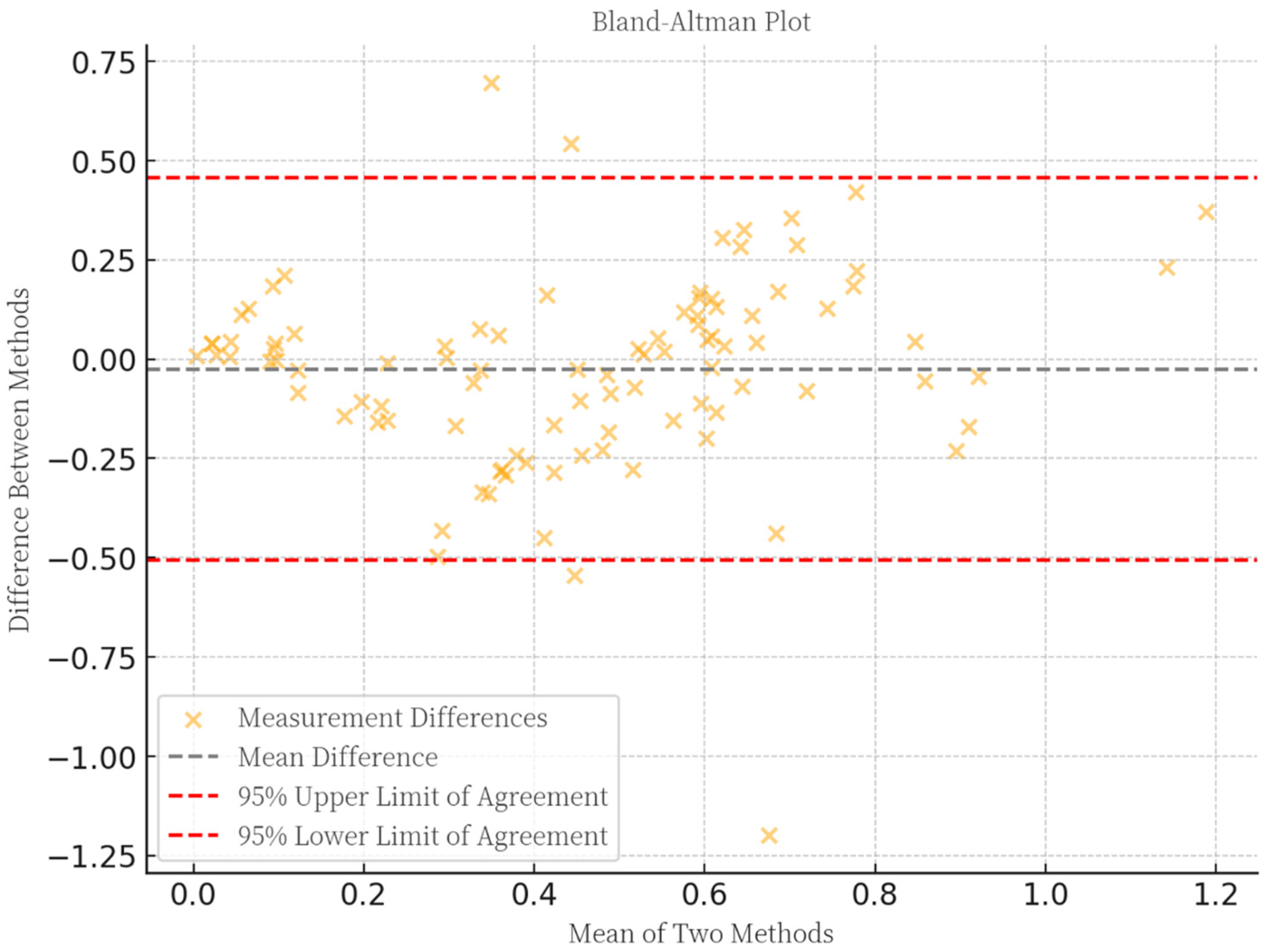
Using 97 exempted ships’ information provided by the maritime authorities to validate the effectiveness of the quantitative inversion of source intensity and fuel sulfur content estimation method. The results represented that the proposed method could effectively replace the carbon balance method in terms of the detection rate of suspected ships and the outlier rate, with a detection rate of 87.63% and an outlier rate of 2.06%, respectively.

(3)

Randomly selecting the operation data for 30 consecutive days to show the actual monitoring effect and evaluate the stability and practicality of this method. Among the 3316 ships, 2743 had their fuel sulfur content detected, with an effective detection rate of 82.72%. In total, 131 ships were suspected of using fuel with high sulfur content, and 111 of them were confirmed to use non-compliant fuel by sampling and detection with portable analytical instruments, with a detection accuracy of 84.73%.

In addition to the challenges of matching peak concentrations with ships and the influence of complex meteorological conditions, other limitations should be noted. First, the monitoring equipment’s coverage is limited to a specific area, which may restrict the detection of emissions from ships operating outside this range. Second, the simplified assumptions in the dispersion model may not fully capture the complexities of real-world dispersion processes. Third, the estimation of fuel consumption rates may be affected by variations in ship load and operational conditions. Addressing these limitations in future studies could further enhance the robustness and applicability of the proposed method.

References

1. Sun, Y.; Zheng, J.; Han, J.; Liu, H.; Zhao, Z. Allocation and reallocation of ship emission permits for liner shipping. Ocean Eng. 2022, 266, 112976. [Google Scholar] [CrossRef]
2. Wu, H.; Li, X.; Wang, C.; Ye, Z. Inverse calculation of vessel emission source intensity based on optimized gaussian puff model and particle swarm optimization algorithm. Mar. Pollut. Bull. 2024, 209, 117117. [Google Scholar] [CrossRef] [PubMed]
3. Zhou, F.; Wang, Y.; Hou, L.; An, B. Air pollutant emission factors of inland river ships under compliance. J. Mar. Sci. Eng. 2024, 12, 1732. [Google Scholar] [CrossRef]
4. Chen, X.; Dou, S.; Song, T.; Wu, H.; Sun, Y.; Xian, J. Spatial-temporal ship pollution distribution exploitation and harbor environmental impact analysis via large-scale AIS data. J. Mar. Sci. Eng. 2024, 12, 960. [Google Scholar] [CrossRef]
5. da Silva, J.N.R.; Santos, T.A.; Teixeira, A.P. Methodology for predicting maritime traffic ship emissions using automatic identification system data. J. Mar. Sci. Eng. 2024, 12, 320. [Google Scholar] [CrossRef]
6. Zhao, J.; Zhang, Y.; Patton, A.P.; Ma, W.; Kan, H.; Wu, L.; Fung, F.; Wang, S.; Ding, D.; Walker, K. Projection of ship emissions and their impact on air quality in 2030 in Yangtze River delta, China. Environ. Pollut. 2020, 263, 114643. [Google Scholar] [CrossRef] [PubMed]
7. International Maritime Organization. Index of MEPC Resolutions and Guidelines related to MARPOL Annex VI. Resolut. MEPC 2021, 328, 76. [Google Scholar]
8. Åström, S.; Yaramenka, K.; Winnes, H.; Fridell, E.; Holland, M. The costs and benefits of a nitrogen emission control area in the baltic and north seas. Transp. Res. Part D Transp. Environ. 2018, 59, 223–236. [Google Scholar] [CrossRef]
9. Ministry of Transport of the People’s Republic of China. Implementation Scheme of the Domestic Emission Control Areas for Atmospheric Pollution from Vessels; Ministry of Transport of the People’s Republic of China: Beijing, China, 2018.
10. Bendl, J.; Saraji-Bozorgzad, M.R.; Käfer, U.; Padoan, S.; Mudan, A.; Etzien, U.; Giocastro, B.; Schade, J.; Jeong, S.; Kuhn, E.; et al. How do different marine engine fuels and wet scrubbing affect gaseous air pollutants and ozone formation potential from ship emissions? Environ. Res. 2024, 260, 119609. [Google Scholar] [CrossRef]
11. Huang, S.; Li, Y. New exploration of emission abatement solution for newbuilding bulk carriers. J. Mar. Sci. Eng. 2024, 12, 973. [Google Scholar] [CrossRef]
12. Anand, A.; Wei, P.; Gali, N.K.; Sun, L.; Yang, F.; Westerdahl, D.; Zhang, Q.; Deng, Z.; Wang, Y.; Liu, D.; et al. Protocol development for real-time ship fuel sulfur content determination using drone based plume sniffing microsensor system. Sci. Total. Environ. 2020, 744, 140885. [Google Scholar] [CrossRef] [PubMed]
13. Cheng, Y.; Wang, S.; Zhu, J.; Guo, Y.; Zhang, R.; Liu, Y.; Zhang, Y.; Yu, Q.; Ma, W.; Zhou, B. Surveillance of SO2 and NO2 from ship emissions by MAX-DOAS measurements and the implications regarding fuel sulfur content compliance. Atmos. Chem. Phys. 2019, 19, 13611–13626. [Google Scholar] [CrossRef]
14. Liu, R.W.; Yuan, W.; Chen, X.; Lu, Y. An enhanced CNN-enabled learning method for promoting ship detection in maritime surveillance system. Ocean Eng. 2021, 235, 109435. [Google Scholar] [CrossRef]
15. Van Roy, W.; Schallier, R.; Van Roozendael, B.; Scheldeman, K.; Van Nieuwenhove, A.; Maes, F. Airborne monitoring of compliance to sulfur emission regulations by ocean-going vessels in the Belgian North Sea area. Atmos. Pollut. Res. 2022, 13, 101445. [Google Scholar] [CrossRef]
16. Van Roy, W.; Van Roozendael, B.; Vigin, L.; Van Nieuwenhove, A.; Scheldeman, K.; Merveille, J.-B.; Weigelt, A.; Mellqvist, J.; Van Vliet, J.; van Dinther, D.; et al. International maritime regulation decreases sulfur dioxide but increases nitrogen oxide emissions in the North and Baltic Sea. Commun. Earth Environ. 2023, 4, 391. [Google Scholar] [CrossRef]
17. Šaparnis, L.; Rapalis, P.; Daukšys, V. Ship Emission measurements using multirotor unmanned aerial vehicles: Review. J. Mar. Sci. Eng. 2024, 12, 1197. [Google Scholar] [CrossRef]
18. Van Roy, W.; Merveille, J.-B.; Scheldeman, K.; Van Nieuwenhove, A.; Van Roozendael, B.; Schallier, R.; Maes, F. The role of belgian airborne sniffer measurements in the MARPOL Annex VI enforcement chain. Atmosphere 2023, 14, 623. [Google Scholar] [CrossRef]
19. Cao, K.; Zhang, Z.; Li, Y.; Xie, M.; Zheng, W. Surveillance of ship emissions and fuel sulfur content based on imaging detection and multi-task deep learning. Environ. Pollut. 2021, 288, 117698. [Google Scholar] [CrossRef]
20. Zhang, Z.; Wang, H.; Cao, K.; Li, Y. Using a convolutional neural network and mid-infrared spectral images to predict the carbon dioxide content of ship exhaust. Remote. Sens. 2023, 15, 2721. [Google Scholar] [CrossRef]
21. Huang, H.; Zhou, C.; Xiao, C.; Wen, Y.; Ma, W.; Wu, L. Identification and detection of high NO x emitting inland ships using multi-source shore-based monitoring data. Environ. Res. Lett. 2024, 19, 044051. [Google Scholar] [CrossRef]
22. Krause, K.; Wittrock, F.; Richter, A.; Schmitt, S.; Pöhler, D.; Weigelt, A.; Burrows, J.P. Estimation of ship emission rates at a major shipping lane by long-path DOAS measurements. Atmos. Meas. Tech. 2021, 14, 5791–5807. [Google Scholar] [CrossRef]
23. Gao, Q. Research on Back-Calculation of Inland Waterway Sailing Ships Exhaust Emission Source Intensity in Gaussian Mode. Master’s Dissertation, Southeast University, Nanjing, China, 2021. [Google Scholar]
24. Liu, J.; Wang, S.; Zhang, Y.; Yan, Y.; Zhu, J.; Zhang, S.; Wang, T.; Tan, Y.; Zhou, B. Investigation of formaldehyde sources and its relative emission intensity in shipping channel environment. J. Environ. Sci. 2024, 142, 142–154. [Google Scholar] [CrossRef]
25. Zhu, Y.; Chen, Z.; Asif, Z. Identification of point source emission in river pollution incidents based on bayesian inference and genetic algorithm: Inverse modeling, sensitivity, and uncertainty analysis. Environ. Pollut. 2021, 285, 117497. [Google Scholar] [CrossRef] [PubMed]
26. Tang, H. Research on Exhaust Gas Diffusion of Ships at Sea based on Gaussian Model. Master’s Dissertation, Southeast University, Nanjing, China, 2021. [Google Scholar]
27. He, Z.; You, L.; Liu, R.W.; Yang, F.; Ma, J.; Xiong, N. A cloud-based real time polluted gas spread simulation approach on virtual reality networking. IEEE Access 2019, 7, 22532–22540. [Google Scholar] [CrossRef]
28. Liu, Y.; Zhang, Y.; Yuan, Y.; Wang, S.; Guo, J.; Wang, L.; Zhou, B. Identification of sulfur content in marine fuel oil based on real-time ship emissions and online monitoring of plumes. Acta Sci. Circumstantiae 2021, 41, 2624–2632. [Google Scholar] [CrossRef]
29. Lotrecchiano, N.; Sofia, D.; Giuliano, A.; Barletta, D.; Poletto, M. Pollution dispersion from a fire using a gaussian plume model. Int. J. Saf. Secur. Eng. 2020, 10, 431–439. [Google Scholar] [CrossRef]
30. Zhao, J.; Li, J.; Bai, Y.; Zhou, W.; Zhang, Y.; Wei, J. Research on leakage detection technology of natural gas pipeline based on modified gaussian plume model and markov chain monte carlo method. Process. Saf. Environ. Prot. 2024, 182, 314–326. [Google Scholar] [CrossRef]
31. Cao, K.; Zhang, Z.; Li, Y.; Zheng, W.; Xie, M. Ship fuel sulfur content prediction based on convolutional neural network and ultraviolet camera images. Environ. Pollut. 2021, 273, 116501. [Google Scholar] [CrossRef]
32. Wu, H.; Wang, C.; Chen, E.; Ye, Z. Development of a spectrum-based ship fuel sulfur content real-time evaluation method. Mar. Pollut. Bull. 2023, 188, 114484. [Google Scholar] [CrossRef]
33. Fu, J. A Forecasting System and Modeling for Diffusion of Ship Exhaust Emission. Master’s Dissertation, Dalian Maritime University, Dalian, China, 2019. [Google Scholar]
34. Sun, J.; Shu, J.; Qiu, B.; Wang, Y.; Wang, Q. An Industry air pollution dispersion system based on Gaussian dispersion model. Available Environ. Pollut. Control. 2005, 7, 50–53. [Google Scholar]
35. Fa, G. Turbulent diffusion-typing schemes: A review. Nucl. Saf. 1976, 17, 68–86. [Google Scholar]
36. George, S.; Nandanan, D.; Muralikrishna, P. Improving accuracy of source localization algorithms using kalman filter estimator. J. Phys. Conf. Ser. 2021, 1921, 12022. [Google Scholar] [CrossRef]
37. Lu, J.; Huang, M.; Wu, W.; Wei, Y.; Liu, C. Application and improvement of the particle swarm optimization algorithm in source-term estimations for hazardous release. Atmosphere 2023, 14, 1168. [Google Scholar] [CrossRef]
38. GB/T 7187.2-2010; Fuel Oil Consumption for Transportation Ships, Part 2: Calculation Method for Inland Ships. Standardization Administration of China: Beijing, China, 2010.
39. Li, S. The Study on Adhesion Skimmer Design. Master’s Dissertation, Dalian Maritime University, Dalian, China, 2011. [Google Scholar]
40. Jalkanen, J.-P.; Brink, A.; Kalli, J.; Pettersson, H.; Kukkonen, J.; Stipa, T. A modelling system for the exhaust emissions of marine traffic and its application in the Baltic Sea area. Atmos. Chem. Phys. 2009, 9, 9209–9223. [Google Scholar] [CrossRef]
41. Jalkanen, J.-P.; Johansson, L.; Kukkonen, J.; Brink, A.; Kalli, J.; Stipa, T. Extension of an assessment model of ship traffic exhaust emissions for particulate matter and carbon monoxide. Atmos. Chem. Phys. 2012, 12, 2641–2659. [Google Scholar] [CrossRef]
42. Chen, D.; Wang, X.; Li, Y.; Lang, J.; Zhou, Y.; Guo, X.; Zhao, Y. High-spatiotemporal-resolution ship emission inventory of China based on AIS data in 2014. Sci. Total. Environ. 2017, 609, 776–787. [Google Scholar] [CrossRef]
43. Bland, J.M.; Altman, D.G. Statistical methods for assessing agreement between two methods of clinical measurement. Lancet 1986, 327, 307–310. [Google Scholar] [CrossRef]
44. Qi, S.; Wang, J.; Zhang, X.; Yang, Z.; Xie, Z.; Li, J. Research on monitoring method of fuel sulfur content of ships in Tianjin port. J. Phys. Conf. Ser. 2021, 2009, 12073. [Google Scholar] [CrossRef]
Figure 1. Schematic diagram of Gaussian plume line source model.
Jmse 13 00690 g001
Figure 2. Methodology flowchart.
Jmse 13 00690 g002
Figure 3. Schematic diagram of equipment layout position and mode.
Jmse 13 00690 g003
Figure 4. Schematic diagram of ship emission diffusion for different emission source heights.
Jmse 13 00690 g004
Figure 5. Schematic diagram of ship emission diffusion for different wind speeds.
Jmse 13 00690 g005
Figure 6. Schematic diagram of ship emission diffusion for different atmospheric stability.
Jmse 13 00690 g006
Figure 7. Bland–Altman results of the proposed method and carbon balance method.
Jmse 13 00690 g007
Figure 8. Results of fuel sulfur content for ships over 30 consecutive days.
Jmse 13 00690 g008