Article

A Weak Signal Detection Method Based on HFER Features in Sea Clutter Background

1
School of Electronic Engineering, Nanjing Xiaozhuang University, Nanjing 211171, China
2
School of Electronics & Information Engineering, Nanjing University of Information Science and Technology, Nanjing 210044, China
3
School of Information Engineering, Nanjing Xiaozhuang University, Nanjing 211171, China
*
Author to whom correspondence should be addressed.
J. Mar. Sci. Eng. 2025, 13(4), 684; https://doi.org/10.3390/jmse13040684
Submission received: 6 March 2025 / Revised: 18 March 2025 / Accepted: 25 March 2025 / Published: 28 March 2025
(This article belongs to the Section Ocean Engineering)

Abstract

:
To address the issue of aliasing between weak signals and sea clutter, we have developed a weak signal detection method leveraging High-Frequency Energy Ratio (HFER) features. This feature detection approach significantly enhances the detection performance of weak signals against the backdrop of sea clutter. By thoroughly examining the echo characteristics that distinguish clutter range gates from target range gates, we transition the analysis from the observation domain to the feature domain, thereby achieving effective discrimination between the two. We analyze the distribution characteristics of high-frequency IMF energy ratios following CEEMD decomposition and construct a weak signal detection network using XGBoost, with the energy ratio as the key feature. The hyperparameters of the network are optimized using the Sparrow Search Algorithm (SSA). We conducted a comparative analysis using the BCD, RAA, TIE, SVM, and multi-feature fusion detection methods. The experimental results showed that the detection probability of the proposed method can reach over 95%, significantly improving the sea surface monitoring and target tracking capabilities of sea radar.

1. Introduction

Sea clutter, which is the backscatter echo resulting from the irradiation of the sea surface by maritime radar systems, poses a significant challenge in radar signal processing. The echoes captured by the radar can be categorized into two types: pure sea clutter and sea clutter containing embedded weak signals [1,2]. The primary objective of this research is to mitigate the impact of environmental noise present in radar echoes, effectively extract the weak signals, and thereby enhance the detection capabilities of maritime radar systems in identifying small targets against the complex sea background. This endeavor aims to bolster the radar’s ability to discern subtle targets, which are often obscured by the overwhelming presence of sea clutter.
In the domain of traditional detection, a suite of features such as amplitude characteristics, fractal dimensions, and time–frequency energy profiles has been employed [3]. Early research endeavors leveraged a spectrum of statistical models—including Rayleigh, lognormal, Weibull, and K-distributions—to elucidate the intricacies of sea clutter [4]. These studies revealed that the amplitude distribution of sea clutter exhibits substantial variation across diverse maritime conditions, primarily attributed to the heterogeneity in radar parameters and marine environmental factors. Although these models have low computational complexity, their corresponding applicability is narrow. The quest for a universal model that encapsulates all existing amplitude models remains unfulfilled, underscoring the complexity and the need for tailored approaches in characterizing sea clutter across various scenarios. Researchers have increasingly integrated nonlinear mathematical analysis techniques into the modeling of sea clutter. Predominantly, these methodologies are categorized into two distinct approaches: one grounded in the principles of fractal chaos theory and the other rooted in time–frequency analysis.
Fractal theory has been extensively applied in the domain of radar signal processing, renowned for its straightforward computation and remarkable efficiency. Li et al. [5] employed Empirical Mode Decomposition (EMD) on sea clutter signals, scrutinized the fractal properties of each Intrinsic Mode Function (IMF), and established a Hurst exponent feature space, thereby facilitating object detection. Building on this, Xing et al. [6] integrated the Complementary Ensemble Empirical Mode Decomposition (CEEMD) with the variable-scale Duffing oscillator, proposing a novel method for weak signal detection. The fractal characteristics of sea clutter are highly sensitive to the Signal-to-Noise Ratio (SNR), posing challenges in differentiating between sea clutter and target signals under low SNR conditions. Sea clutter manifests fractal behavior within a specific time-scale scale-free interval [7], which is subject to variations in radar parameters, maritime conditions, and polarization states. Furthermore, estimation inaccuracies and limited observation durations within this scale-free interval can also compromise detection performance.
The sea clutter analysis method that leverages time–frequency characteristics can extract more detailed information through appropriate time–frequency transformations. This approach primarily employs techniques such as the short-time Fourier transform, Wigner–Ville distribution, smooth pseudo-Wigner–Ville distribution, and fractional Fourier transform [8]. These methods enable the extraction of target-corresponding features on a two-dimensional plane, thereby facilitating detection. Xiong et al. [9] proposed a radar clutter reconstruction model based on the singularity power spectrum and instantaneous singularity exponent distribution. However, these tools struggle to balance time–frequency resolution with computational efficiency. Although detection performance has significantly improved compared to statistical models, the computational complexity remains a concern.
With the advent of machine learning, a variety of nonlinear detection methodologies have emerged, including Support Vector Machines (SVMs), Extreme Learning Machines, Radial Basis Functions, and Hidden Markov Chains, often in conjunction with neural networks, for the detection of weak signals in the maritime environment [10,11,12,13,14]. Xu et al. [15] delved into the impact of sea clutter polarization modes on detection efficacy, leveraging polarization information to enhance object detection capabilities. Li et al. [16] introduced a multi-objective adaptive detection algorithm that integrates an error self-correcting extreme learning machine with the Fractional Fourier Transform. Their experimental results, while validated through simulation data, were noted to lack corroboration from actual measurement data. Li et al. [17] proposed a spatial–temporal graph neural network detector to detect marine targets. Experimental results on two public radar databases for marine target detection validate the effectiveness and superiority of the proposed detector against several popular marine target detection methods in terms of detection performance and real-time test efficiency.
Despite the end-to-end automatic feature extraction achieved by the data-driven ground sea clutter classification methods mentioned, several limitations persist: (1) the methods fail to effectively capitalize on intra- and inter-class sample information; (2) they require a substantial volume of high-quality, balanced labeled samples, which incurs significant computational complexity and time costs; and (3) the models are characterized by a multitude of parameters, necessitating extensive training periods and entailing high maintenance costs in practical applications. Consequently, there is a compelling need for in-depth research into the relationships among sea clutter samples and the development of more lightweight ground sea clutter classification models that address these challenges.
We have chosen the CEEMD algorithm to extract features from sea clutter, thereby enhancing the efficiency and accuracy of machine-learning models. The CEEMD algorithm, an extension of the Ensemble Empirical Mode Decomposition (EEMD), was initially designed for denoising time-series data [18,19,20,21,22]. Zhang et al. [23] introduced a rainfall prediction approach grounded in CEEMD–fine composite multi-scale entropy, which was integrated into a stacking ensemble learning framework and applied to predict monthly precipitation levels in the Xixia region. Dai et al. [24] utilized CEEMD to capture the characteristics of cavitation, and the ensuing decomposition results were fed into a 12-layer deep residual shrinkage network for cavitation identification training, effectively enhancing the identification of cavitation at various stages of centrifugal pumps. The comparison of various performance indicators between the proposed method and related research is shown in Table 1.
Through this comparison, it can be seen that, although existing methods have made progress in certain aspects, there are still limitations, such as the insufficient adaptability to complex sea conditions, low computational efficiency, or dependence on large amounts of high-quality data. In this study, we harness the adaptive decomposition attributes of the CEEMD to dissect the impact of weak signals on the frequency and energy architecture of IMFs. We introduce a methodology for extracting HFER features, which are pivotal for discerning subtle signals obscured by sea clutter. We encompass the design of an XGBoost network tailored to ascertain the category of the extracted feature parameters, with the hyperparameter ensemble optimized via the SSA. This approach significantly enhances the nuanced cognitive capacity for interpreting sea clutter and adeptly accomplishes the detection of weak signals embedded within this complex backdrop.

2. Sea Clutter Characteristics After CEEMD Decomposition

The CEEMD method adds a set of positive and negative white noise signals to the sea clutter for EMD decomposition, and combines the decomposition results to obtain the final IMF. CEEMD can suppress reconstruction errors caused by white noise while maintaining good decomposition performance. The steps to implement the CEEMD algorithm for denoising sea clutter are as follows:
(1) Add n groups of auxiliary white noise to the original sea clutter in the form of positive and negative pairs:
M 1 M 2 = 1 1 1 1 S N
where: S is the original sea clutter; N is auxiliary noise; and M 1 and M 2 are the composite signals after adding positive and negative paired noises, respectively, so the number of signals in the set is 2 n .
(2) EMD decomposition is performed on each signal in the set, and each signal gets a group of IMF components. The j IMF component of the i signal is expressed as I M F i j .
(3) The decomposition result is obtained by combining multiple components:
I M F j = 1 2 n i = 1 2 n I M F i j
Therefore, the signal S can be expressed as L IMF components, along with residual components R es :
S = j = 1 L I M F j + R es
CEEMD decomposition was performed on the first 1000 sampling points of group #17 sea clutter data. The article “The Sea Clutter De-noising Based on Ensemble Empirical Mode Decomposition” [22] shows that the first 1000 sampling points of sea clutter can represent the difference between signal and noise, we use Matlab R2016a to present this result, as shown in Figure 1:
Figure 1 illustrates that, due to the comparable complexity between target range gates and clutter range gates, the number of IMF components derived from their CEEMD decomposition is identical. This observation underscores the challenge in discriminating targets from clutter range gates.
Upon comparing the amplitudes of the high-frequency IMF in the first half and the low-frequency IMF in the second half, it is evident that, in the CEEMD decomposition map of the clutter range gate, the overall fluctuation amplitude of the high-frequency IMF aligns with that of the low-frequency IMF. As a result, the y-axis coordinates are relatively smaller compared to the decomposition diagram of the target range gate. In contrast, within the CEEMD decomposition diagram of the target range gates, except for certain mutation points, the overall amplitude of the high-frequency IMF in the first half is generally lower than that of the low-frequency IMF in the second half, showing an ascending trend.
The distribution characteristic observed is attributed to the influence of floating debris—which are the sources of weak signals—on the high-frequency component of sea clutter after CEEMD decomposition. Targets exhibit a narrow frequency spectrum, concentrating their primary energy in the lower frequencies, specifically in the second half of the IMFs. In contrast, the frequency spectrum of sea clutter is broader, leading to a dispersion of energy across various IMF orders. As a result, the proportion of energy in the high-frequency IMFs is greater for the clutter range gates compared to the target range gates. Additionally, offshore spikes contribute to the increased energy in the high-frequency IMFs within the clutter range gates.
Leveraging these decomposition features, we propose employing the energy ratio of the IMFs to differentiate between high- and low-frequency components. By calculating the energy proportion occupied by the first E IMFs across the entire signal, we can identify the energy proportion with the highest discriminative power as the detection feature. This approach transitions the analysis of target and clutter range gates from the observation space to the feature space.
Figure 1 demonstrates the outcome of CEEMD decomposition on both target and clutter range gates, yielding eight IMF components. For preliminary experiments, we adopted the median approach and calculated the energy ratio of the first five IMF components, as depicted in Figure 2.
Figure 2 demonstrates a significant difference in the total energy ratio from IMF1 to IMF5 between distance gates with and without targets, which can be easily separated by a threshold, as indicated by the dashed line in the figure. Under sea condition #17, the energy ratios of distance gates with targets are all below 0.01, while those without targets are all above 0.1, differing by an order of magnitude.
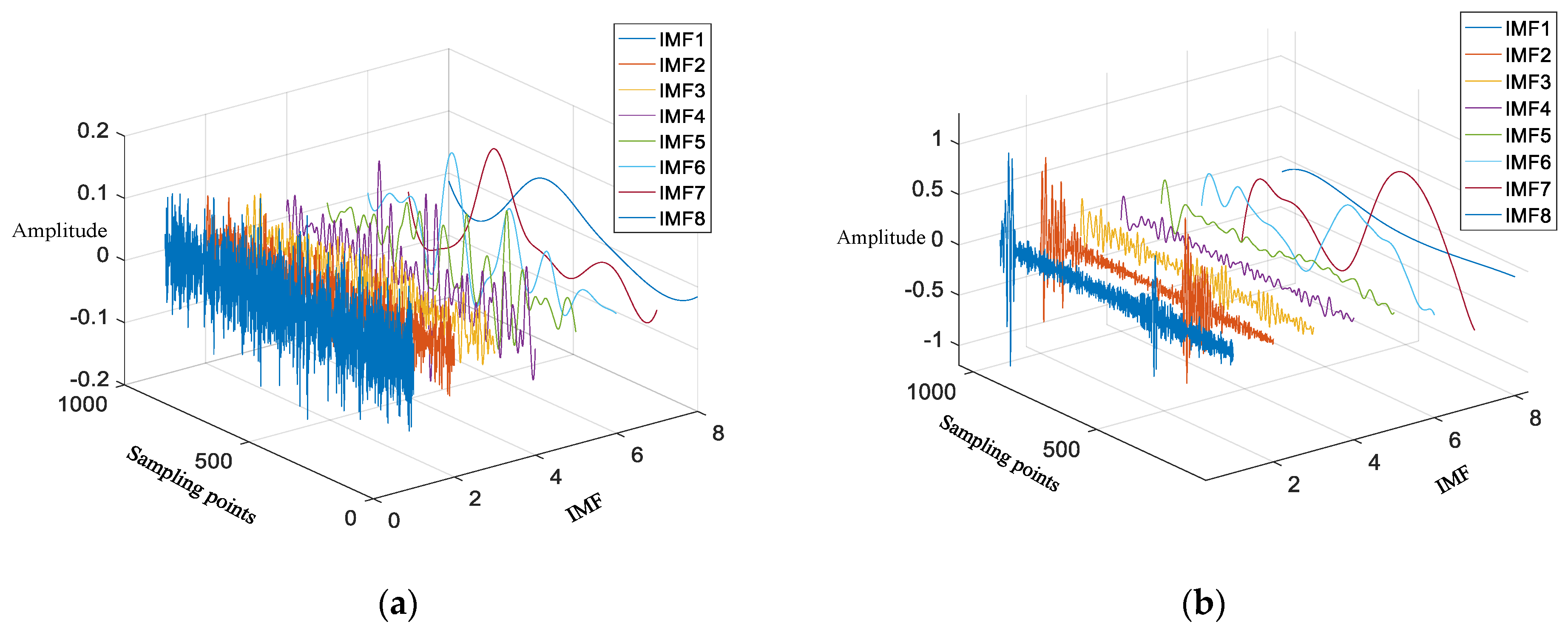
To enrich the experimental subjects, experiments were conducted using sea condition #54, which has a higher signal-to-noise ratio. The CEEMD decomposition diagrams of the first 1000 points for both target and non-target distance gates are displayed in Figure 3.
Figure 3 illustrates that the amplitude range difference between the high-frequency IMF of the clutter distance gate and the low-frequency IMF is not pronounced, whereas a significant difference is observed after the decomposition of the target distance gate. The amplitude range of the high-frequency IMF is considerably smaller than that of the low-frequency IMF, aligning with the characteristics observed under sea condition #17.
Adhering to the principle of CEEMD decomposition and considering the data performance of these two types of sea conditions, the energy characteristics of the IMFs decomposed by CEEMD align with the target distribution traits of sea clutter. These characteristics can be effectively utilized as discriminative features for the classification of sea clutter.
For the #54 sea condition, the total energy proportion of the top four IMF groups across all range gates was calculated, and the distribution curve of the total energy proportion, ordered by the distance gates, is presented in Figure 4.
Figure 4 reveals that the energy ratio for the seventh, eighth, ninth, and tenth distance gates with targets remains beneath 0.01, whereas the energy ratio for the clutter range gates is no less than 0.07, marking a discrepancy of at least sevenfold. This substantial difference substantiates the efficacy of the proposed HFER feature in readily distinguishing target distance gates. Figure 3, with its amplitude differences in IMFs, further corroborates that, under conditions of high SNR and superior data quality, the energy characteristics of IMFs decomposed by CEEMD are reflective of the inherent traits of sea clutter.
We calculate the average energy ratio of the two types of range gates of the first half of the high-frequency IMF under the five groups of sea conditions, as shown in Table 2. The separability of the proposed features is demonstrated by the order of magnitude difference between the two.
Table 2 demonstrates that, across the five sets of sea conditions, the average energy ratio of the high-frequency IMF for the clutter gate is significantly higher compared to the target gate, with a difference of an order of magnitude. This substantial disparity underscores the robust separability of the proposed HFER feature, rendering it apt for detecting weak signals amidst sea clutter.
For groups #17, #54, and #40 in Table 2, which correspond to sea conditions with a high SNR, the energy disparity between the clutter gate and the target gate exceeds sevenfold. Notably, in group #17, where the sea clutter boasts superior data quality, this difference escalates to over 25 times, affirming the HFER feature’s efficacy in distinctly differentiating between the target and clutter gates.
Groups #26 and #310, indicative of low SNR sea conditions, exhibit a less pronounced difference, yet maintain a minimum twofold gap. As the SNR diminishes, the multiplicative difference decreases as well, evidencing the HFER feature’s heightened efficacy in high signal-to-noise ratio environments, yet retaining its viability for low SNR scenarios. This renders the HFER feature extraction method a practical and applicable solution for engineering applications.

3. HFER Feature Extraction of Weak Signals Under Sea Clutter

In Section 2, we conducted an analysis of the energy distribution within the high-frequency IMFs across various distance gates. Our findings confirmed that the energy ratio of the high-frequency IMF aligns with the distribution characteristics of sea clutter targets, suggesting its potential as a feature for weak signal detection. This alignment serves as a distinguishing criterion, allowing for the differentiation between clutter and target signals within the complex maritime environment. The HFER feature extraction method, which encapsulates this principle, is formalized in Equation (4):
H = I M F 1 2 + + I M F X 2 S 2
Among the various components, IMF1 to IMFX denote the set of IMFs that effectively distinguish between target and clutter range gates. S signifies the sea clutter prior to decomposition, while H stands for the extracted HFER features. The selection of high-frequency signals is confined to the first half of the IMF set, with no definitive method for demarcation. Leveraging the validated distribution characteristics of the high-frequency IMF energy ratio, this section delves into the high-frequency spectrum of the IMFs, establishing a theoretical foundation for the detection of weak signals in practical engineering scenarios amidst a sea clutter background.

3.1. HFER Feature Extraction of Sea Clutter Using CEEMD Decomposition of Even IMF

We conducted CEEMD decomposition on the initial 1000 sampling points of the Group #17 sea condition, yielding a total of eight IMFs. We then computed the energy ratios for the first E IMF components, where E spans from 1 to 8, as illustrated in Figure 5.
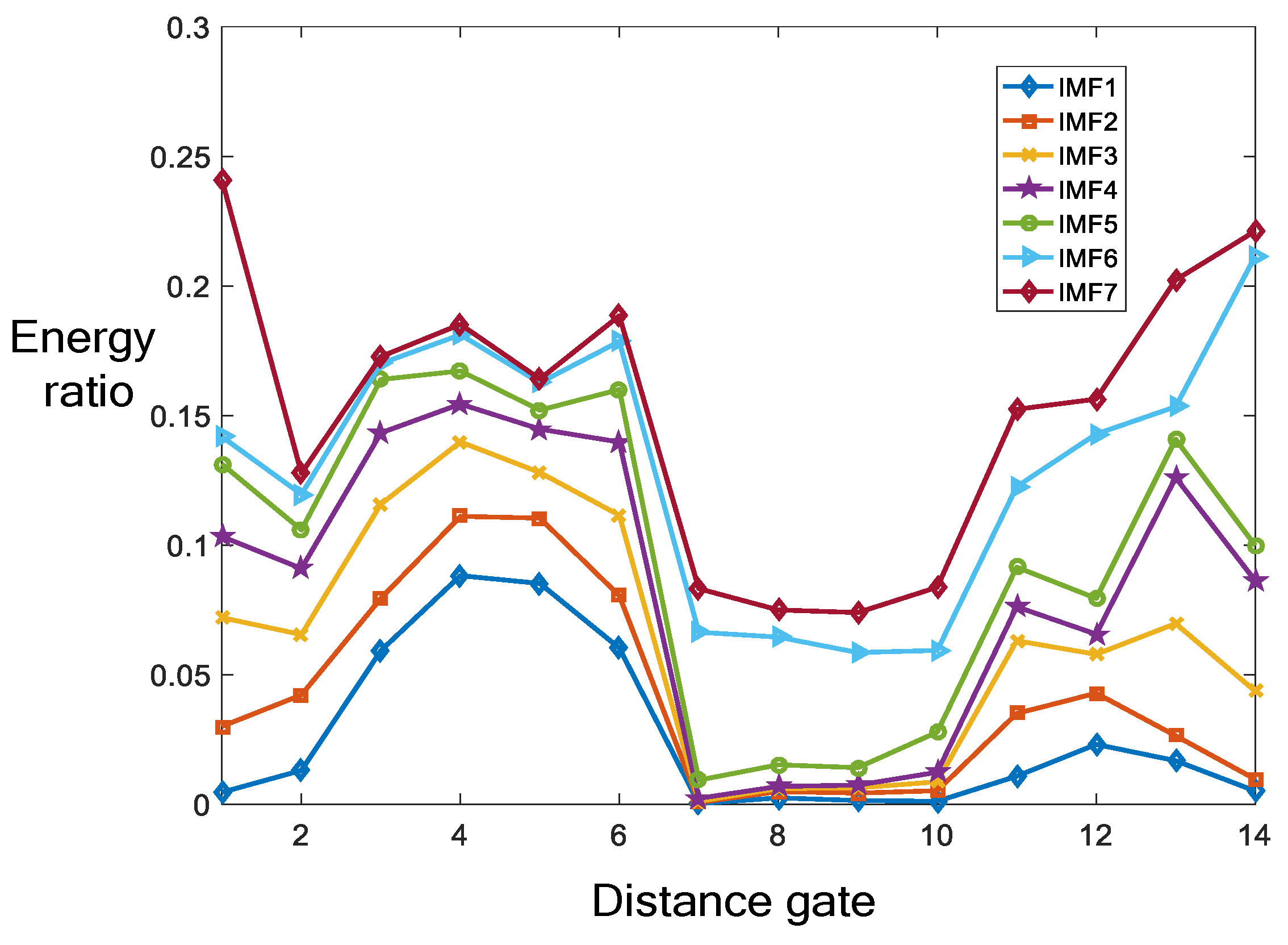
Under sea condition #17, among the 14 range gates, the eighth, tenth, and eleventh range gates are secondary target range gates, while the ninth range gate is the primary target range gate. As shown in Figure 5, each IMF resulting from CEEMD decomposition exhibits a certain trend in target distribution, with a lower energy proportion in the eighth to eleventh range gates and a higher energy proportion in the other range gates.
This is due to the influence of floating spheres on the high-frequency component of sea clutter within the range gate that contains the target. Floating spheres have a smaller radar cross-section and a narrower spectrum, resulting in the primary energy distribution in the latter half of the IMFs. In contrast, the spectrum of sea clutter is broader, with energy more evenly distributed across each order of IMF, and a higher proportion of high-frequency IMFs. Additionally, the presence of offshore spikes can lead to an increased energy gain in the high-frequency IMFs of the clutter range gates, gradually widening the gap between the target and non-target range gates.
The energy ratios of the first and second IMF components are relatively low in clutter range gates and exhibit minimal differences compared to those with targets; thus, these two components are not considered. The energy ratio curves of the sixth to eighth IMF components show a noticeable increase in the ninth range gate, which contains the main target, and are larger than those in the secondary target range gates; hence, these three components are also disregarded. The remaining IMF3, IMF4, and IMF5 components, when combined with Figure 5, reveal that the distribution curve of IMF5 differs significantly between the two types of range gates. The ninth range gate, containing the main target, has the lowest energy ratio and the most distinct target distribution characteristics.
To quantitatively analyze the HFER features most suitable for weak signal detection under sea clutter backgrounds, we calculated the ratio of the minimum energy in the clutter range gates to the maximum energy in those with targets, as shown in Table 3. The IMF set with the highest ratio was selected.
As presented in Table 3, under sea condition #17, the energy ratio set of each IMF exhibits an initial increase followed by a decrease, with the minimum differential ratio being 0.7467. Notably, the energy ratio of the clutter distance gate is consistently lower than that of the target distance gate, suggesting that the HFER feature does not provide separability at this juncture. However, the energy ratio of the first five IMFs demonstrates the most significant difference between the distance gates with and without targets, with a ratio of up to 2.94 times. This finding corroborates that employing the energy ratio of the first five IMFs as the HFER feature to distinguish between distance gates with and without targets is the most effective approach.
We analyzed the reasons for this variation by selecting two extreme points. The energy proportion of IMF1 among all IMFs showed essentially no difference between the clutter range gate and the target range gate. This is due to the adaptive decomposition characteristic of CEEMD. For each range gate, the IMF1 component decomposed represents pure noise, which is composed of radar measurement noise and dynamic noise from sea wind and sea waves. This noise has a similar impact on both the clutter range gates and the target range gates.
The energy ratios of IMF1 to IMF5 demonstrate an increasing trend, ranging from 1.1691 to 2.9407 times. Beyond the peak difference at IMF5, the decomposed IMF components tend to rearrange towards the original signal, with the energy ratio differences diminishing, returning to the indistinguishable sea clutter.
In summary, when the number of CEEMD decompositions is an even number of E , the energy ratio of the top E 2 + 1 IMFs is selected as the classification feature.

3.2. HFER Feature Extraction of Sea Clutter Using CEEMD Decomposition of Odd IMF

We conducted CEEMD decomposition on the dataset from group #54, yielding a total of seven IMFs. The energy ratios for the initial 1 through 7 IMFs were computed and are depicted in Figure 6. Within the 14 range gates of the sea condition for group #54, the seventh, ninth, and tenth range gates are identified as secondary target range gates, while the eighth range gate is recognized as the main target range gate.
As depicted in Figure 6, it is observed that the sea condition data of Group #54 are of high quality with a high SNR, and the distribution of energy ratios for each IMF is relatively clear. However, in the energy ratio curves of IMF1 and IMF2, the amplitude at the end is low, and the difference from the target distance gate is small, leading to the decision not to consider these two components as characteristics of sea clutter. Upon observing the curves of IMF6 and IMF7, there is a minor decrease at the target distance gate. A comprehensive comparison of the curve variations among the seven IMF components reveals that the energy ratios of IMF3 and IMF4 are more consistent with the target distribution characteristics.
The floating ball on the sea surface is located at the eighth distance gate, and the seventh to tenth distance gates are also affected. Sea clutter generally has a wide spectral distribution, with energy spread across multiple IMF components. However, the presence of a target with a narrow spectral signature disrupts this distribution, leading to a reduction in the high-frequency energy proportion.
We further analyzed the HFER features that are most suitable for weak signal detection in the presence of sea clutter. The ratio of the minimum energy in clutter range gates to the maximum energy in target range gates was calculated, as shown in Table 3. The IMF set with the largest ratio was selected.
From Table 4, it can be seen that the IMF ratio of sea conditions in #54 also shows a trend of first increasing and then decreasing. The energy ratio of IMF1~IMF3 and IMF1~IMF4 has a significant difference in the target and clutter distance gates, both of which are more than five times, demonstrating good separability, and can be used as classification IMF sets. However, IMF3 has the largest difference, reaching 5.498 times. For precise classification, the energy ratio of the first three IMFs after CEEMD decomposition among all IMFs was selected as the classification feature for the #54 group of sea situation signals.
Based on this, it can be concluded that, in the case of processing an odd number of E IMFs decomposed by CEEMD, the energy ratio of the first E 1 2 IMFs is used as the sea clutter characteristic signal for classification, thereby completing the task of weak signal detection.
Further research on the extraction of HFER features under low signal-to-noise ratio conditions was conducted. The #310 group data with a SNR of 2.1 dB were decomposed using CEEMD, yielding seven IMF components, and the energy ratios of the first 1 to 7 IMFs were calculated. Then, we compare the ratio of the minimum energy of each IMF set in the clutter distance gate to the maximum energy of the target distance gate, as shown in Table 5:
According to Table 5, under the low SNR #310 sea conditions, the difference multiple of IMF1, IMF2, IMF5, IMF6, and IMF7 are all less than 1, indicating that the energy ratio of clutter distance gates in these IMF sets is even smaller than that of target distance gates, with the lowest being only 0.1427, which does not have obvious separability. The reason is that the data quality affects the feature separation ability.
The energy ratio of the first three IMFs has the largest difference between the distance gates with and without targets, and can still differ by nearly twice even in cases of poor data quality. This proves that using the energy ratio of the first three IMFs as the HFER feature for dividing the distance gates with and without targets is the most appropriate.
It was found in conjunction with sea condition group #54 that, when an odd number of E IMF components were obtained from CEEMD decomposition, the energy ratio of the first E 1 2 IMFs was selected as the feature for classification.
We analyzed the IMF characteristics of sea clutter and the segmentation method for high-frequency IMF. The implementation steps of the HFER feature extraction method for weak signal detection are as follows:
(1) We perform CEEMD decomposition on the sea clutter to obtain a series of E IMF components: I M F 1 , I M F 2 , , I M F E .
(2) When E is an odd number, calculate Formula (6) as the HFER-CEEMD feature.
H = I M F 1 2 + + ( I M F E 1 2 ) 2 S 2
When E is even, calculate Formula (7) as the HFER-CEEMD feature.
H = I M F 1 2 + + ( I M F E 2 + 1 ) 2 S 2
In Formulae (5) and (6), S represents the sea clutter before decomposition, and H represents the extracted HFER features. The dimension of the HFER feature H obtained is consistent with the CEEMD decomposition of sea clutter, yielding 14 HFER-CEEMD features corresponding to each sea condition, categorized into features with targets and features without targets.

4. Design of SSA–XGBoost Weak Signal Detection Network

In the detection of weak signals in the background of sea clutter, there are two states of sea clutter: one is to simultaneously receive weak signals and sea clutter, while the other is only sea clutter. The task of sea surface target detection is to determine whether there are weak signals in the received sea clutter, which is simplified as a binary classification problem between clutter units and target units. Therefore, the detection problem is essentially a binary hypothesis test.
After extracting HFER features, we use the XGBoost model with a high computational efficiency and low risk of overfitting to optimize the hyperparameters of XGBoost through SSA. We design an SSA–XGBoost target detection network to transform the problem of detecting weak signals in the sea clutter background into a feature classification problem with or without targets.

4.1. HFER Feature Segmentation Method

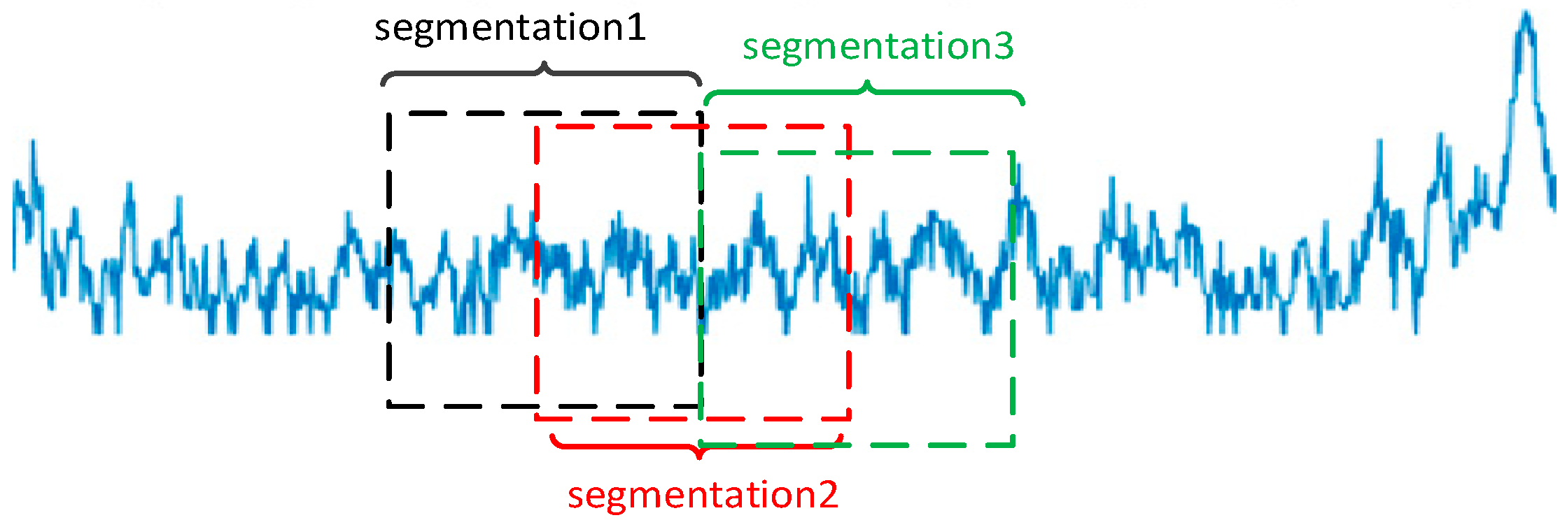
There are a total of 14 distance gates for sea clutter in each sea situation, among which 3–4 distance gates contain targets, and the rest are pure sea clutter distance gates, resulting in an imbalance in the number of clutter samples and signal samples. To enrich the dataset and enhance the classification ability of the network, the data are expanded and processed using a fixed-step data collection method. The energy ratio sample data are subdivided into small-scale samples of different types, and the clutter data are segmented into 128 sampling points. To balance the samples, the target data are segmented according to a sliding window, as shown in Figure 7:
We assume the number of sampling points for segmentation is n ; that is, the data from the 1st to the n th sampling point are segmented into a new data segment, and the data from the n 2 th to the n + n 2 th sampling point become the second data segment, and so on, to enrich the number of classification samples.

4.2. HFER Feature Classification Network Structure Based on XGBoost

XGBoost is a supervised model composed of a series of CART trees. Figure 8 shows the process of the XGBoost classification network for weak signals undera sea clutter background using five pieces of high-frequency IMF energy ratio data and two tree structures:
XGBoost can automatically utilize the central processing unit for multi-threaded parallel computing [25]. XGBoost’s new loss function is second-order-differentiable and incorporates a regularization term to find the optimal solution as a whole, in order to balance the decrease in the loss function and the complexity of the model, improve classification accuracy, and avoid overfitting.
Assuming the model has k decision trees, namely,
y ^ i = k = 1 K f k ( x i ) , f k F ,
the loss function is
O b j = i = 1 n l ( ( y i , y ^ ( t 1 ) ) + f t ( x i ) ) + Ω ( f t ) + C
Among them, y ^ ( t 1 ) represents retaining the model prediction from the previous t 1 round, and F = f ( x i ) = ω q ( x i ) , ω R T , q : R m 1 , 2 , , T is the function space composed of classification regression trees; ω is the leaf weight; T is the number of leaf nodes on the tree; q is the structure of each tree, that is, the mapping of sample instances to corresponding leaf node indices; and each f k corresponds to an independent tree structure q k and leaf weights ω k , and C is a constant term.
Perform Taylor second-order expansion on the objective function and define two variables for ease of calculation. As shown below,
g i = y ^ i ( t 1 ) l ( y ^ i ( t 1 ) , y i )
h i = y ^ i ( t 1 ) 2 l ( y ^ i ( t 1 ) , y i )
The objective function can be changed to Equation (11):
O b j ( t ) i = 1 n [ l ( y i , y ^ ( t 1 ) ) + g i f t ( x i ) + 1 2 h i f t 2 ( x i ) ] + Ω ( f t ) + C
When training the model, the objective function can be represented by Equation (12):
O b j ( t ) = j = 1 t [ ( i I j g i ) w j + 1 2 ( i I j h i + λ ) w j 2 ] + γ T
Define Equation (13):
O b j ( t ) i = 1 n [ l ( y i , y ^ ( t 1 ) ) + g i f t ( x i ) + 1 2 h i f t 2 ( x i ) ] + Ω ( f t ) + C
Substitute Equation (13) into Equation (12) to obtain Equation (14):
O b j ( t ) = j = 1 t [ G j w j + 1 2 ( H j + λ ) w j 2 ] + γ T       = 1 2 j = 1 T G j 2 H j + λ + γ T
The smaller the value of O b j ( t ) , the better the performance of the constructed network. The principle of XGBoost is to calculate the first derivative g i and second derivative h i of each node and sample, and then sum up the samples contained in each node to obtain G j and H i .
Finally, the objective function can be obtained by traversing the decision tree nodes. While it is difficult for general ensemble learning algorithms to specifically list all regression trees, the XGBoost algorithm uses the gradient boosting strategy, constantly adding new trees during the training process to fit the previous learning errors.

4.3. SSA Optimization of HFER Feature Classification Network Based on XGBoost

During the training process, the classification performance of the XGBoost model is easily affected by hyperparameters. The hyperparameter information of the XGBoost model that affects the classification results is shown in Table 6:
From Table 6, it can be seen that the selection of numerous hyperparameters determines the training effectiveness of the XGBoost model. Improper selection can seriously affect the classification results. Therefore, it is necessary that we optimize the hyperparameter set of the XGBoost network to obtain a model that is suitable for the training samples and to improve the final detection probability.
During the process of foraging, sparrow populations can be divided into two types: discoverers and followers. Discoverers are responsible for discovering food in the population and informing the entire sparrow population of the next foraging area and direction, while followers obtain food through the information obtained by discoverers.
Individuals in sparrow populations will monitor the behavior of other individuals in the population, and attackers in the population will compete with individuals with a high intake for food resources to increase their predation rate. In addition, when sparrow populations become aware of danger, they will engage in anti-predatory behavior. Based on this intelligent role assignment, the sparrow search algorithm has the advantages of a strong global search ability, short optimization time, and fast convergence speed, and is suitable for optimizing weak signal detection networks under a sea clutter background. The XGBoost hyperparameter set for optimizing the classification of HFER sea clutter features using the sparrow search algorithm can be represented by the following mathematical model.
Equation (15) represents the assumed sparrow population:
X = x 1 1 x 1 2 x 1 d x 2 1 x 2 2 x 2 d x n 1 x n 2 x n d
In Equation (15), n represents the number of sparrows; and d represents the dimension of the variable that needs to be optimized.
The fitness value of sparrows is expressed using Equation (16):
F x = f ( [ x 1 , 1 x 1 , 2 x 1 , d ] ) f ( [ x 2 , 1 x 2 , 2 x 2 , d ] ) f ( [ x n , 1 x n , 2 x n , d ] )
In Equation (16), the value of each row f in F x represents the fitness value of each individual.
During the search process, the order in which sparrows obtain food is related to their fitness level, with sparrows that prioritize obtaining food having higher fitness. The leader of the sparrow population is called an explorer. Explorers are responsible for searching for food and providing directions for other sparrows in the population to search for food, thus having the largest range for searching for food.
When the sparrow population is in the absence of predators, the search direction of the explorer is arbitrary. Once a predator appears around the population, the explorer will lead followers to move away from the predator.
The formula for updating the position of the explorer, which is the fitness value, is shown in Equation (17):
X i , j t + 1 = X i , j t exp ( i α i t e r max ) , R 2 < S T X i , j t + Q L , R 2 S T
In Equation (17), t represents the current number of iterations; i t e r max represents the maximum number of iterations; X i , j represents the position information of the i-th sparrow in the j-th dimension; α is a random number and α 0 , 1 ; R 2 represents the warning value R 2 0 , 1 ; S T represents the safety value S T 0.5 , 1 ; Q is a random number that follows a normal distribution; and L is a 1 × d matrix where all elements are 1.
When R 2 S T , it indicates the presence of danger and predators in the area; when it is the other way around, it indicates that the area is safe and there are no predators present.
In the entire sparrow population, the ratio of explorers to followers is fixed and unchanging. If followers can find better food, they can become explorers, and vice versa. Due to the fact that only explorers in the sparrow population have better foraging environments and larger foraging ranges, followers will constantly observe the explorers’ situation and compete with them for food in order to obtain better food. If followers succeed in the competition, they will obtain the explorers’ food instead of searching for food in farther places. The follower position update formula, Formula (18), is as follows:
X i , j t + 1 Q exp ( X w o r s t t X i , j t i 2 ) , i > n 2 X P t + 1 + X i , j X P t + 1 A + L , i n 2
In Equation (18), X w o r s t represents the global worst position; X P represents the best position among the current discoverers; A is an 1 × d -dimensional matrix with only 1 and −1 elements, and A + = A T ( A A T ) 1 ; and n represents the total number of sparrows.
When i > n 2 , it indicates that the fitness of the i th follower is low and they have not obtained food, and they need to fly to other directions to search for food.
Vigilantes are randomly generated, so their positions are also random. The number of vigilantes is generally set at 10% to 20% of the entire sparrow population. When vigilantes detect predators around them, the peripheral sparrows will quickly fly to a safe place to obtain a better search environment. The internal sparrows will move within a safe area to reduce the probability of being preyed upon by predators. The location update formula, Formula (19), for the alert is as follows:
X i , j t + 1 = X b e s t t + β X i , j t X b e s t t , f i > f g X i , j t + K X i , j t X w o r s t t ( f i f w ) + ε , f i = f g
In Equation (19), X b e s t represents the current global optimal position; β represents the step size and follows a normal distribution; K is a random number K 1 , 1 ; f i represents the fitness value of the current sparrow individual; f g represents the current global optimal fitness value; f w represents the current global worst fitness value; and ε is a constant used to avoid the denominator appearing as 0. When f i > f g , it means that the peripheral sparrows have discovered predators; when it is the other way around, it means that the sparrow inside has discovered a predator.
The steps for classifying sea clutter HFER features using SSA–XGBoost are as follows:
(1) Data preprocessing normalizes the HFER feature sequence to [ 1 , 1 ] , with the aim of limiting the input sequence to a certain range and solving problems such as inability to converge or slow convergence caused by special sample HFER data. Divide the training set and the testing set.
(2) Determine and initialize the hyperparameter groups Learning_rate, Max_depth, Colsample-bytree, and Subsample to be optimized in the XGBoost network, and initialize the relevant parameters of the sparrow search algorithm.
(3) Calculate the individual fitness value f i of sparrows, and sort and select the current global best fitness value f g and worst fitness value f w , as well as their corresponding positions f g and X b e s t .
(4) Update the position of sparrows, based on the warning value R 2 and safety value S T , and update the position of discoverers, joiners, and sparrows that are aware of danger. Obtain the current global best fitness value f g and the corresponding global best position X b e s t .
(5) Select the global optimal solution after reaching the maximum number of iterations; otherwise, iterate again.
(6) Take the optimal output solution as the hyperparameter set to be optimized for XGBoost.
(7) Input the test set samples into the optimal XGBoost model and output the classification results.
The flowchart of weak signal detection under a sea clutter background based on the SSA–XGBoost algorithm is shown in Figure 9:
5. Experiments and Analysis

To test the practicality of the frequency-ordered wavelet packet multi-threshold denoising method, we conducted experiments using measured sea clutter data. The sea clutter data used in this article are the IPIX radar sea clutter data from McMaster University in Canada. The main parameters of the IPIX radar are shown in Table 7.

5.1. Experiment on Detecting Weak Signals in Sea Clutter Based on HFER Features

Comparing the direct use of sea clutter for XGBoost classification, extracting HFER features for XGBoost classification, and optimizing the detection rate of the XGBoost network using SSA after extracting HFER features, experiments were conducted using high SNR #17 and #54 sea condition data and low SNR #280 sea condition data with only 4.1 dB. We use Python3.6 to conduct experiments. The experimental results are shown in Figure 10:
From Figure 10, it can be seen that the detection rate of XGBoost classification for sea clutter is around 80%, and the detection rate for the #54 group of sea conditions reaches 94.5%. This is because the SNR of the #54 group of sea conditions is high and the data quality is good, while the detection rates for the other two groups of sea conditions are not ideal. This indicates that the XGBoost network can initially classify sea clutter, but the detection rate does not meet the requirements of weak signal detection.
To improve the detection rate, CEEMD decomposition was used to explore the distribution of sea clutter at different frequency scales. It was found that the energy ratio of the high-frequency part of the IMF after CEEMD decomposition matched the target characteristics. It was treated as a feature for XGBoost classification, and the detection rate after classification reached around 95%, which was 10% higher than that of featureless classification. This indicates that the proposed HFER feature conforms to the motion law of sea clutter data and is suitable for detecting weak signals in the background of sea clutter.
On this basis, using SSA to optimize the hyperparameter group in the XGBoost network, the detection rate of the optimized classification network can be improved by 3%, indicating that the proposed SSA network optimization algorithm can further enhance the detection capability.
After feature extraction, network design, and optimization algorithms were proposed, the detection rate gradually increased, and a detection rate of 96.7% was achieved even in the low SNR of #280 sea conditions. This proves that the proposed classification network based on HFER features is suitable for detecting weak signals in sea clutter under various sea conditions.

5.2. Comparison of IPIX Radar Sea Clutter Feature Detection Experiments

Set the false alarm rate to 10–3 and conduct comparative experiments with various detection methods that have gradually developed, such as the Box Counting Dimension (BCD) method [26], the Relative Average Amplitude (RAA) method, the Temporal Information Entropy (TIE) method [27], the SVM method [11], and the multi-feature fusion detection method [28]. The experimental results are shown in Figure 11:
From Figure 11, it can be seen that, even in the detection of the #17 sea conditions with a high SNR, the detection rate of each comparison algorithm is less than 50%. The proposed HFER–XGBoost feature extraction method has the highest detection probability, reaching 97.8%, which is a qualitative improvement and far exceeds other comparison algorithms. The proposed features conform to the target distribution characteristics of sea clutter, once again verifying the energy ratio curve mentioned earlier. At the same time, it also proves that the designed sea surface target classification network based on HFER features is very suitable for detecting weak signals under sea clutter background.
Further comparison was made using the #54 group of sea conditions with a high SNR, and the experimental results are shown in Figure 12:
As shown in Figure 12, the detection probabilities of all algorithms under sea condition #54 have increased to some extent. This is because the data quality of group #54 is relatively high, and the average detection rate of the comparison algorithms can reach 63.2%. However, the detection accuracy of the proposed HFER feature extraction and classification method reaches 98.3%, which is superior to the other comparison algorithms and is close to the detection probability of the multi-feature method.
The multi-feature detection method combines three features of the sea clutter pulse amplitude deviation ratio, frequency peak to average ratio, and local shape, and finally uses support vector machine for classification. The proposed algorithm only extracts one feature, and the calculation is far less complicated than that of multi-feature detection. The detection probability still reaches 98.3%, indicating that the proposed method reduces the computational complexity while ensuring the detection probability.
The above two comparative experiments focus on high SNR sea conditions. To further analyze the practicality of HFER features under low SNR conditions, comparative experiments were conducted on the data of sea condition #280 with a low SNR. The experimental results are shown in Figure 13:
As shown in Figure 13, compared with the sea condition #54 data with a higher SNR, the classification accuracy of various classification methods for the sea condition #280 data with a low SNR has decreased to some extent. However, the classification accuracy of the proposed method is still higher than that of the comparison algorithms. For sea conditions with poor data quality, the proposed method can achieve a classification accuracy of 96.7%, which is at a relatively high level. Considering that only one feature is extracted, the ability to classify targets effectively demonstrates that the proposed feature conforms to the characteristics of sea clutter. Moreover, this also proves that the designed XGBoost classification network is suitable for the detection of weak signals in the presence of sea clutter.

5.3. Experimental Comparison of Fynmeet Radar Sea Clutter Feature Detection

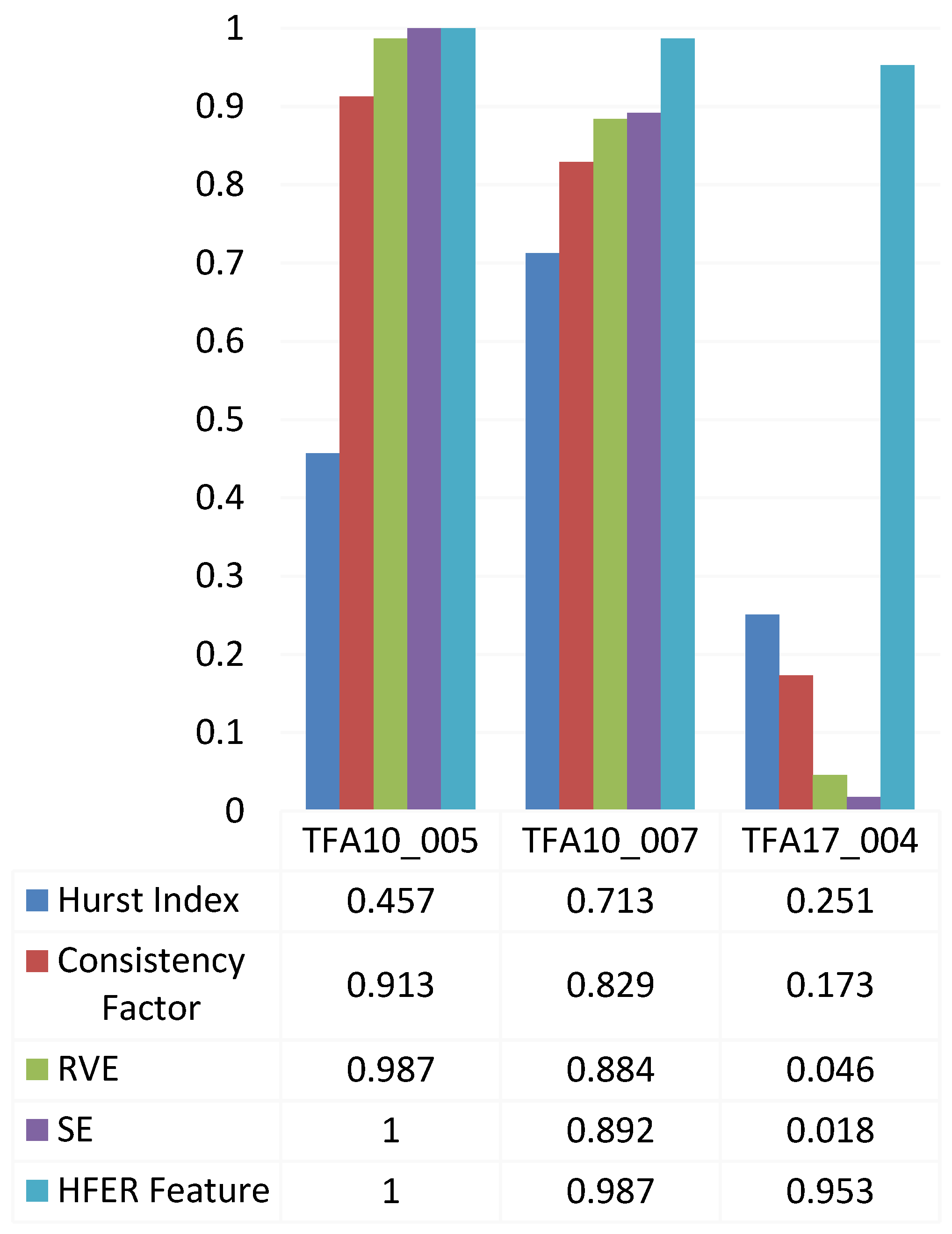
To verify the applicability of the HFER feature extraction method, three sets of sea clutter data were measured using the South African Fynmeet radar. Although the detection targets of the South African Fynmeet radar and the Canadian IPIX radar are different, they both belong to the category of radar echoes containing weak signals caused by sea surface targets. The sea situation numbers are TFA10_005, TFA10_007, and TFA17_004. Without conducting preliminary analysis and discussion, we directly use Equations (2) and (3) for feature extraction, and apply the improved SSA–XGBoost for target classification. We compare the experimental results with several effective feature extraction methods, including the Hurst exponent [5], consistency factor [29], RVE [30], and Sample Entropy [31]. The experimental results are shown in Figure 14:
The purpose of proposing HFER features is to study a universal, non-tedious, and well-separable classification feature for sea clutter and weak signals. Thus, when the feature extraction method and classification network are proposed, and validation experiments are conducted on data from other sources, without any analysis or discussion of radar characteristics, the feature extraction formula is directly applied to verify the universality and detection performance of the proposed HFER features.
From Figure 14, it can be seen that the proposed HFER features have significantly improved detection performance compared to the comparative methods, and are suitable for detecting weak signals in sea clutter backgrounds under different conditions. For the two types of sea clutter with good data quality, TFA10_005 and TFA10_007, only the Hurst exponent feature detection method has a lower detection rate of 45.7% and 71.3%, respectively. The detection performance of the other comparison methods is better, reaching over 80%. Especially for the TFA10_005 sea clutter, except for the Hurst feature detection method, the detection rate is very high. The sample entropy detection achieved a detection rate of 100%, which is consistent with the detection rate of the proposed HFER feature, proving that the data quality of this sea situation is very good. For the TFA10_007 sea clutter, the detection rate of the proposed feature reaches 98.7%, which is more than 10% higher than other comparison algorithms, indicating that HFER features have a good separability for sea clutter with good data quality.
The HFER feature is proposed based on the characteristics of the IPIX radar. Although the installation environment, illuminated sea area, and detection object of the IPIX radar and Fynmeet radar are different, the weak signal detection method based on the HFER feature can still achieve good detection results, indicating that the proposed HFER feature conforms to the laws of sea clutter motion and has universality.

6. Conclusions

Traditional single-dimensional features cannot effectively distinguish targets from clutter. Multi-feature detection methods combining multiple features emerged, improving detection performance but requiring extensive analysis and complementary features. These methods are computationally intensive and unsuitable for practical engineering applications.
We analyzed sea clutter under various sea conditions and found that CEEMD decomposition reveals distinct energy distributions in high-frequency IMFs for target and clutter range gates. This led to the development of an HFER feature extraction algorithm, which maximizes the separation between target and clutter gates. Using XGBoost and SSA for classification and hyperparameter optimization, our method achieves over 96% accuracy in weak signal detection under different sea conditions, outperforming other methods. The HFER feature’s generalization ability was verified using Fynmeet radar data, showing excellent detection performance without complex analysis. This method can detect weak signals from various targets and is applicable in different sea conditions and SNRs.
Our study integrates the characteristics of sea clutter with advanced deep-learning networks to achieve satisfactory detection results. However, the innovations are primarily focused on the data processing level and the application of deep learning. Future research could explore changes in the structure and framework of deep-learning networks, or even propose entirely new neural networks tailored for chaotic sea clutter detection based on the characteristics of sea clutter. By leveraging the strengths of deep learning in pattern recognition, feature extraction, and rapid technological innovation, this approach can contribute to the development of target detection technology in maritime environments.

Author Contributions

Conceptualization, Y.Y.; methodology, Y.Y. and Y.S.; software, Z.Q.; validation, H.X.; formal analysis, Y.Y.; investigation, Y.S.; resources, H.X.; data curation, Y.Y.; writing—original draft preparation, Y.Y. and Z.Q.; writing—review and editing, Y.S. and H.X.; visualization, Y.Y.; supervision, Y.S.; project administration, Y.Y.; funding acquisition, Y.Y. All authors have read and agreed to the published version of the manuscript.

Funding

This research was financially supported by the Natural Science Research Funding Project for Ordinary Universities in Jiangsu Province (Grant No. 23KJD510007), National Natural Science Foundation of China (Grant No. 62171228), and The Youth Special Project of the University-level Research Program at Nanjing Xiaozhuang University (Grant No. 2022NXY27), and The APC was funded by Natural Science Research Funding Project for Ordinary Universities in Jiangsu Province (Grant No. 23KJD510007), and The Youth Special Project of the University-level Research Program at Nanjing Xiaozhuang University (Grant No. 2022NXY27).

Data Availability Statement

The original data presented in this study are openly available by the Communications Research Laboratory at McMaster University in Canada, where Professor S. Haykin is based, at http://soma.ece.mcmaster.ca/ipix/dartmouth/, accessed on 5 January 2025.

Acknowledgments

We are grateful to the School of Electronics & Information Engineering at Nanjing University of Information Science and Technology for providing a solid foundation for our research. We also thank the School of Electronic Engineering at Nanjing Xiaozhuang University, for their continuous support throughout this research. We sincerely appreciate the constructive comments from the anonymous reviewers, which have significantly enhanced the quality of this manuscript.

Conflicts of Interest

The authors declare no conflicts of interest.

Glossary

The following abbreviations and symbols are used in this manuscript:
Abbreviations
HFERHigh-Frequency Energy Ratio
SSASparrow Search Algorithm
EMDEmpirical Mode Decomposition
IMFIntrinsic Mode Function
CEEMDComplementary Ensemble Empirical Mode Decomposition
SNRSignal-to-Noise Ratio
SVMSupport Vector Machines
EEMDEnsemble Empirical Mode Decomposition
BCDBox Counting Dimension
RAARelative Average Amplitude
TIETemporal Information Entropy
Symbols
S sea clutter
N noise
M 1 positive paired noises
M 2 negative paired noises
I M F i j j IMF component of the i signa
R es residual components
H HFER-CEEMD feature
y ^ ( t 1 ) model prediction from the previous t 1 round
ω leaf weight
T number of leaf nodes on the tree
q structure of each tree
O b j ( t ) objective function
d dimension of the variable
t current number of iterations
i t e r max maximum number of iterations
X i , j position information of the i-th sparrow in the j-th dimension
α random number
R 2 warning value
S T safety value
Q random number
X w o r s t global worst position
X P best position
X b e s t current global optimal position
β step size
K random number
f i fitness value of the current sparrow individual
f g global optimal fitness value
f w global worst fitness value

References

  1. Li, Q.; Chen, Y.; Dang, X.W.; Yin, H.C.; Xu, G.G.; Chen, X. Sea clutter prediction based on fusion of Fourier transform and graph neural network. Int. J. Remote Sens. 2024, 45, 6544–6571. [Google Scholar] [CrossRef]
  2. He, H.F.; Li, Z.; Zhang, X.; Jia, J.G.; He, Y.M. Characteristic Description and Statistical Model-Based Method for Sea Clutter Modeling. Remote Sens. 2024, 16, 4429. [Google Scholar] [CrossRef]
  3. Linghu, L.X.; Wu, J.J.; Jeon, G.; Wu, Z.S.; Shi, M. Sea Clutter Feature Prediction and Parameters Inversion Using Deep Learning Model. IEEE Trans. Ind. Inform. 2023, 19, 8374–8383. [Google Scholar] [CrossRef]
  4. Ding, M.Y.; Li, Y.C.; Quan, Y.H.; Guo, L.; Xing, M.D. A Novel Reconstruction Method of K-Distributed Sea Clutter with Spatial–Temporal Correlation. Sensors 2020, 20, 2377. [Google Scholar] [CrossRef]
  5. Kuang, H.X.; Yang, L.X. A Sea-Surface-Zoning Method Based on Fractal Characteristics. Sensors 2022, 22, 4761. [Google Scholar] [CrossRef]
  6. Xing, H.Y.; Wu, H.; Liu, G. Variable-Scale Duffing Oscillator Method for Weak Signal Detection. Acta Electron. Sin. 2020, 48, 734–742. [Google Scholar]
  7. Sun, J.; Xing, H.Y.; Wu, J.J. Chaotic Small Signal Detection Method Based on IA-SVM Model. J. Detect. Control 2020, 42, 119–125. [Google Scholar]
  8. Shi, S.N.; Shui, P.L. Sea-Surface Floating Small Target Detection by One-Class Classifier in Time-Frequency Feature Space. BMC Complement. Altern. Med. 2018, 56, 6395–6411. [Google Scholar] [CrossRef]
  9. Xiong, G.; Wang, L.J.; Yu, W.X. Radar sea clutter reconstruction based on statistical singularity power spectrum and instantaneous singularity exponents distribution. BMC Complement. Altern. Med. 2021, 59, 5687–5697. [Google Scholar] [CrossRef]
  10. Chen, X.X.; Wu, J.J.; Guo, X. Prediction of sea clutter characteristics by deep neural networks using marine environmental factors. Environ. Dev. Sustain. 2022. [Google Scholar] [CrossRef]
  11. Shui, P.L.; Zhang, L.X.; Bai, X.H. Small Target Detection in Sea Clutter by Weighted Biased Soft-Margin SVM Algorithm in Feature Spaces. IEEE Sens. J. 2024, 24, 10419–10433. [Google Scholar] [CrossRef]
  12. Bai, X.H.; Xu, S.W.; Guo, Z.X.; Shui, P.L. Graph-Based Maximum Connected-Component Learning Algorithm for Small Target Detection in Maritime Radars. IEEE Trans. Aerosp. Electron. Syst. 2025, 61, 250–265. [Google Scholar] [CrossRef]
  13. Su, N.Y.; Chen, X.L.; Guan, J.; Huang, Y. Maritime target detection based on radar graph data and graph convolutional network. IEEE GRSL 2022, 19, 4019705. [Google Scholar] [CrossRef]
  14. Schreiber, F.M.; Angelliaume, S.; Guerin, C.A. Modeling the polarization ratio in the upper microwave band for sea clutter analysis. IEEE TGRS 2021, 59, 6323–6335. [Google Scholar] [CrossRef]
  15. Shuwen, X.U.; Jia, P.U. Floating amall tergeta detection in sea clutter based on four-polarization-channel fuaion. J. Signal Process. 2017, 33, 324–329. [Google Scholar]
  16. Li, Q.Z.; Zhai, Y.J.; Niu, J. Adaptive detection of multi-targets of HFSWR based on ES-ELM and FRFT. Chin. J. Radio Sci. 2020, 35, 270–279. [Google Scholar]
  17. Wang, X.; Cui, G.L.; Wang, Y.M.; Zhao, W.J.; Xiong, K. Marine Target Detection via Spatial Temporal Graph Neural Network. IEEE Trans. Instrum. Meas. 2025, 74, 2505514. [Google Scholar] [CrossRef]
  18. Wang, P.J.; Wu, J.; Wei, Y.; Li, T.Y. CEEMD-MultiRocket: Integrating CEEMD with Improved MultiRocket for Time Series Classification. Electronics 2023, 12, 1188. [Google Scholar] [CrossRef]
  19. Gu, J.; Peng, Y.X. An improved complementary ensemble empirical mode decomposition method and its application in rolling bearing fault diagnosis. Digit. Signal Process. 2021, 113, 103050. [Google Scholar] [CrossRef]
  20. Gao, K.P.; Liu, S.L.; Su, C.X.; Zhang, Q. A multi-stage learning method for excavation torque prediction of TBM based on CEEMD-EWT-BiLSTM hybrid network model. Measurement 2025, 247, 116766. [Google Scholar] [CrossRef]
  21. Liu, H.J.; Yu, X.; Fang, H.Y. A Study on Locating Two Leaks in Water Supply Pipelines Based on CEEMD-SVD-FCMSS. IEEE Sens. J. 2025, 25, 5304–5318. [Google Scholar] [CrossRef]
  22. Xing, H.Y.; Zhu, Q.Q. The Sea Clutter De-noising Based on Ensemble Empirical Mode Decomposition. Acta Electron. Sin. 2016, 44, 1–7. [Google Scholar]
  23. Zhang, X.Q.; Xiao, Y.M.; Zhu, G.Y.; Shi, J.W. A coupled CEEMD-BiLSTM model for regional monthly temperature prediction. Environ. Monit. Assess. 2023, 195, 379. [Google Scholar] [CrossRef] [PubMed]
  24. Dai, C.; Hu, S.Y.; Zhang, Y.H.; Chen, Z.Y.; Dong, L. Cavitation state identification of centrifugal pump based on CEEMD-DRSN. Environ. Monit. Assess. 2023, 55, 1507–1517. [Google Scholar] [CrossRef]
  25. Chen, Z.; Jiang, F.; Cheng, Y.; Gu, X.; Liu, W.; Peng, J. Xgboost classifier for ddos attack detection and analysis in sdn-based cloud. In Proceedings of the 2018 IEEE International Conference on Big Data and Smart Computing (BigComp), Shanghai, China, 15–17 January 2018. [Google Scholar] [CrossRef]
  26. Zhang, J.P.; Zhang, Y.S.; Xu, X.Y.; Li, Q.L.; Wu, J.J. Estimation of the Sea Clutter Inherent Doppler Spectrum from Shipborne S-Band Radar surface radar echo. Chin. Phys. B 2020, 29, 068402. [Google Scholar]
  27. Leibovici, D.G.; Claramunt, C. On Integrating Size and Shape Distributions into a Spatio-Temporal Information Entropy Framework. Entropy 2019, 21, 1112. [Google Scholar] [CrossRef]
  28. Xue, C.L.; Cao, F.; Sun, Q.; Qing, J.Q.; Feng, X.W. Sea-surface weak target detection based on multi-feature information fusion. J. Syst. Eng. Electron. 2022, 44, 3338–3345. [Google Scholar]
  29. Shi, Y.L.; Xie, X.Y.; Li, D.C. Range Distributed Floating Target Detection in Sea Clutter via Feature-Based Detector. IEEE Geosci. Remote Sens. Lett. 2016, 13, 1847–1850. [Google Scholar] [CrossRef]
  30. Shui, P.L.; Li, D.C.; Xu, S.W. Tri-feature-based detection of floating small targets in sea clutter. IEEE Trans. Aerosp. Electron. Syst. 2014, 50, 1416–1430. [Google Scholar] [CrossRef]
  31. Jiang, R.; Li, L.N.; Sun, Q.; Hong, S.Z.; Gao, J.J.; Xu, X.H. Entropy Metrics of Radar Signatures of Sea Surface Scattering for Distinguishing Targets. Remote Sens. 2021, 13, 3950. [Google Scholar] [CrossRef]
Figure 1. CEEMD decomposition diagrams under sea condition #17: (a) decomposition diagram of clutter range gate; and (b) decomposition diagram of target range gate.
Jmse 13 00684 g001
Figure 2. The total energy ratio of the first five IMFs under sea condition #17.
Jmse 13 00684 g002
Figure 3. CEEMD decomposition diagrams under sea condition #54: (a) decomposition diagram of clutter range gate; and (b) decomposition diagram of target range gate.
Jmse 13 00684 g003
Figure 4. IMF energy ratio at different distance gates of the #54 sea conditions.
Jmse 13 00684 g004
Figure 5. Energy ratios of each IMF under sea conditions #17.
Jmse 13 00684 g005
Figure 6. Energy ratios of each IMF under sea conditions #54.
Jmse 13 00684 g006
Figure 7. Data segmentation.
Jmse 13 00684 g007
Figure 8. Calculation process of XGBoost classification network.
Jmse 13 00684 g008
Figure 9. Flow chart of weak signal detection based on SSA–XGBoost algorithm.
Jmse 13 00684 g009
Figure 10. Comparison of SSA–XGBoost algorithm optimization.
Jmse 13 00684 g010
Figure 11. Comparison of detection probability under sea conditions #17.
Jmse 13 00684 g011
Figure 12. Comparison of detection probability under sea conditions #54.
Jmse 13 00684 g012
Figure 13. Comparison of detection probabilities under sea condition #280.
Jmse 13 00684 g013
Figure 14. Comparison of detection probability of sea clutter by Fynmeet radar.
Jmse 13 00684 g014
Table 1. Comparison of performance indicators between the proposed method and related research.
Research MethodFeature ExtractionDetection PerformanceComputational ComplexityLimitations
Traditional Statistical ModelsAmplitude characteristics:
Rayleigh, lognormal, Weibull, and K-distributions
Limited; struggles with complex maritime conditionsLowLack of a universal model; sensitive to changes in maritime conditions
Fractal Chaos TheoryFractal dimensions, Hurst exponentGood performance under high SNR conditionsMediumPerformance drops under low SNR; sensitive to parameter changes
Time–Frequency AnalysisShort-time Fourier transform, time-frequency energy profiles, etc.Enhanced feature extraction; improved detection performanceHighBalancing time–frequency resolution with computational efficiency is challenging
Machine-Learning MethodsSVM, ELM, RBF, etc.Significant performance improvement; data-drivenMediumRequires large volumes of high-quality labeled data; high model complexity
Deep-Learning MethodsNeural networks, spatio-temporal graph neural networksHigh performance; strong adaptabilityVery HighHigh training cost; often lacks validation with real-world data
Our Approach (HFER + XGBoost)High-Frequency Energy Ratio feature extraction; XGBoost for classificationHigh performance; effective for weak signal detectionLowFurther validation needed to assess generalizability across different scenarios
Table 2. Average energy ratio of two types of distance gates for high-frequency IMF in the first half of five sea conditions.
Average Energy Proportion#17#54#40#26#310
Clutter distance gate0.55360.08160.23660.35190.1093
Target distance gate0.02210.00540.03210.07290.0528
Difference multiple25.0515.117.374.8272.07
Table 3. High-frequency IMF energy ratios of the two types of distance gates under sea condition #17.
IMF1IMF2IMF3IMF4IMF5IMF6IMF7
#171.16910.74671.15142.31332.94072.77051.7272
Table 4. High-frequency IMF ratios of two types of distance gates under sea conditions #54.
IMF1IMF2IMF3IMF4IMF5IMF6IMF7
#541.87621.85385.49805.31732.85481.80201.5255
Table 5. High-frequency IMF ratio of two types of distance gates under sea conditions #310.
IMF1IMF2IMF3IMF4IMF5IMF6IMF7
#3100.14270.63261.91440.98750.82510.85790.3710
Table 6. Hyperparameters of XGBoost.
Hyperparameter NameHyperparameter MeaningDefault Value
Learning_rateLearning rate, step size when updating weights in each iteration0.3
Max_depthThe maximum depth of a tree, the larger the value, the easier it is to overfit3
Colsample_bytreeThe proportion of features used in training to all features0.5
SubsampleThe proportion of data used for training to the entire training set1
Table 7. Main parameters of IPIX radar.
Parameter
Radar transmission frequency9.39 GHz
Polarization modeHH/VV/HV/VH
Pulse power8 kW
Pulse width200 ns
Antenna height30 m
Antenna gain45.7 dB
Antenna diameter2.4 m
Antenna typeparabolic shaped
Distance resolution30 m
Disclaimer/Publisher’s Note: The statements, opinions and data contained in all publications are solely those of the individual author(s) and contributor(s) and not of MDPI and/or the editor(s). MDPI and/or the editor(s) disclaim responsibility for any injury to people or property resulting from any ideas, methods, instructions or products referred to in the content.