1. Introduction
Seafloor substrate is a crucial component of marine geographical information, and seafloor substrate classification plays an important role in marine engineering, seabed mineral resource development, and marine habitat research [
1]. In marine engineering and infrastructure development, preliminary investigations of seabed substrate conditions in project areas are essential. For instance, during submarine cable or fiber-optic cable installation, sandy or gravelly substrates are more suitable for cable burial due to their mechanical stability and trenching feasibility, whereas rocky terrains require avoidance or specialized engineering treatments to mitigate abrasion risks. In offshore hydrocarbon and mineral exploration, substrate composition critically influences resource distribution patterns. Sandy sediments, characterized by high porosity and permeability, often serve as hydrocarbon reservoirs, while cohesive clay layers may act as impermeable cap rocks, sealing hydrocarbon accumulations. Similarly, the distribution of marine metallic mineral resources, such as polymetallic nodules and rare-earth-enriched muds, exhibits strong correlations with substrate types and depositional environments. Regarding marine ecological conservation, seabed substrate heterogeneity directly governs the spatial distribution of benthic ecosystems. Specific substrates support distinct biological communities: coral reefs thrive on hard substrates (e.g., bedrock or biogenic carbonates), mollusk populations dominate muddy sediments, and seagrass beds preferentially colonize sandy or mixed substrates. Systematic substrate mapping thus provides a scientific basis for delineating ecologically sensitive zones and establishing marine protected areas.
Traditional substrate classification methods, such as coring or grab sampling, involve field sampling, which not only incurs high costs and takes considerable time but also struggles to cover large areas of the seafloor. With the advancement of seafloor acoustic detection technologies, different substrate types produce varying responses to acoustic signals, allowing for the rapid acquisition of a large amount of seafloor substrate information. As a result, substrate classification based on seafloor acoustic data has become a hot topic in seafloor substrate classification research [
2]. Many researchers have demonstrated that seafloor acoustic data can effectively be used for classifying seafloor sediments.
Common seafloor acoustic detection methods include multi-beam echo sounding, side-scan sonar, and sub-bottom profiling. Both multi-beam echo sounding and side-scan sonar can obtain seafloor depth values and backscatter intensity values for multiple measurement points within a strip-covered area. Compared to side-scan sonar, multi-beam technology can provide more accurate geographical location data, while sub-bottom profiling offers a smaller data coverage range. The principle of seafloor substrate classification based on multi-beam backscatter data is that different seafloor substrate types can reflect varying backscatter intensities. By using the backscatter data, a backscatter intensity grayscale image can be constructed. Seafloor substrate classification can then be performed based on features such as texture or backscatter intensity from the grayscale image [
3].
Some studies have demonstrated the effectiveness of seabed substrate classification based on multi-beam backscatter data [
4,
5]. Traditional methods for seabed substrate classification using multi-beam backscatter data mainly rely on manual classification combined with actual sampling. Although this approach saves a significant amount of time and human resources compared to extensive actual sampling, there is still room for improvement in classification efficiency. The advent of CNNs has made significant progress in image classification. Famous networks include LeNet [
6], AlexNet [
7], GoogLeNet [
8], and VGG [
9]. LeNet is one of the pioneering convolutional neural networks, originally designed for handwritten digit recognition and achieving great classification results in that task. LeNet first combined a convolutional layer and a pooling layer, two novel components of neural networks; proposed a new image processing method; and implemented end-to-end training using a backpropagation algorithm, which optimized the step of manual feature design required by traditional methods. Moreover, the network is simple and utilizes fewer computational resources, allowing for decent classification results even with ordinary devices in a short period of time. LeNet-5 is the most famous and effective version of the LeNet series. AlexNet is a classic convolutional neural network proposed in 2012 for the ImageNet image classification competition. Compared to LeNet, it is more complex, with more convolutional and pooling layers. With its deep network structure, data augmentation, ReLU, and other technical innovations, it achieved outstanding results in the ImageNet large-scale visual recognition competition and received widespread recognition from scholars in related fields. GoogLeNet, also known as Inception v1, was proposed by the Google team in 2014 and won first place in the Classification Task of the ImageNet competition that year. Its biggest innovation is the unique Inception module, which combines convolutional kernels and pooling layers of different sizes to automatically learn and select the most appropriate feature extraction method. The introduction of the Inception module enabled GoogLeNet to adopt a deeper network structure while maintaining a small parameter count, achieving excellent classification performance while consuming fewer computational resources. VGG, proposed by the VGG at Oxford University, is widely used in image classification and object detection tasks. Its network structure is simple and direct, and it achieved impressive results in the ImageNet competition. However, due to its large number of model parameters, it is prone to overfitting when the dataset is small. Since seabed substrate images are relatively scarce compared to general images, we require a good data augmentation method.
As is well known, not only the VGG network but also other deep learning models require large datasets for effective training. However, obtaining a substantial amount of seabed sonar data for deep learning training is time-consuming, costly, and challenging. Therefore, the task of dataset expansion is particularly important. Common data augmentation methods include geometric transformations, image modifications, etc. While these methods have some benefits, they are limited and struggle to generate datasets with various features. The emergence of GANs [
10] addresses this issue. Since their introduction, GANs have found increasing applications in fields such as computer vision, natural language processing, and human–computer interaction [
11]. GANs are primarily composed of two components: a generator module and a discriminator module. The generator produces fake samples from a random noise vector, while the discriminator receives both real and generated samples and outputs a probability indicating how likely the sample is to be real. Through this adversarial process, the generator continuously improves the quality of the generated samples in order to better deceive the discriminator. Compared to traditional data augmentation methods, GANs can generate large datasets with various features. Deep convolutional generative adversarial networks (DCGANs) [
12], a variant of GANs, utilize convolutional neural networks to construct both the generator and discriminator. This enables the network to effectively capture image features, generating more realistic and detailed images. Compared to traditional GANs, DCGANs produce higher-quality images and exhibit better training stability.
This paper combines CNNs for seabed sediment classification based on small-sample multi-beam backscatter data, achieving high classification accuracy while significantly reducing labor and time. The contributions of this study are as follows: (1) seabed sediment classification using CNNs on small-sample multi-beam backscatter data; (2) improvement of the traditional DCGAN by incorporating a de-normalization module to enhance the quality of generated images; (3) application of a DCGAN to augment multi-beam backscatter data, addressing the issue of scarcity of seabed sediment images in multi-beam backscatter data.
2. Materials and Methods
2.1. Data Acquisition and Processing
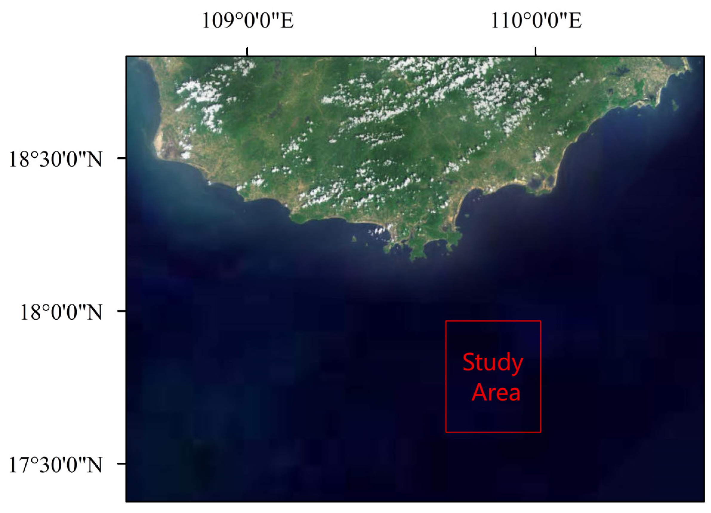
The study area is located on the northern continental shelf edge of the South China Sea, as shown in
Figure 1. The area features a rich variety of seabed sediment types and significant sediment type variations, making it ideal for seabed sediment classification research. An EM302 multi-beam echo sounding system, installed on the vessel, with a frequency of 300 kHz and 256 beams per ping, was used for data collection. The survey area included a 45 km long and 620 m wide survey line, with the seabed sloping from northwest to southeast, where the water depth gradually increases from 90 m to 210 m. For full coverage of the study area by the multi-beam echo sounding system, gravity core sampling was conducted at 53 designated stations. The multi-beam backscatter data were processed using CARIS11.3 software to generate seabed sonar images. Ground truth samples were collected to accurately assess the sediment types, and training samples were extracted near the confirmed stations to create training and validation datasets for network model training.
2.2. Convolutional Neural Networks
CNNs have achieved remarkable success in the field of image classification due to their high computational efficiency, strong generalization ability, and ability to automatically learn and extract useful features from images, eliminating the need for manual feature extraction. Therefore, in this study, a CNN-based approach was used to perform automatic seabed sediment classification using small-sample multi-beam backscatter data. Four networks, LeNet, AlexNet, GoogLeNet, and VGG, have been proven to deliver excellent performances in image classification tasks. Among them, the LeNet network achieved remarkable classification results in handwritten digit recognition, while AlexNet, GoogLeNet, and VGG networks have all performed exceptionally well in the ImageNet competition.
This paper selected the LeNet-5 model from the LeNet network series. The network consists of an input layer, convolutional layers, pooling layers, fully connected layers, and an output layer. The combination of convolutional and pooling layers enables effective extraction of textural and structural features from images, achieving excellent classification performance even with a small number of parameters. The network architecture begins with an input layer receiving 1 × 32 × 32 grayscale images. The initial convolution layer employs six 5 × 5 convolutional kernels with stride 1 and padding 2, followed by sigmoid activation to introduce nonlinear transformations, enabling the network to learn complex functional mappings. Subsequent average pooling performs spatial downsampling to compress feature dimensions and reduce the computational complexity. The second convolutional layer utilizes sixteen 5 × 5 kernels with stride 1 and zero padding, similarly activated through sigmoid nonlinearity before further dimensionality reduction via average pooling. Finally, a fully connected layer transforms the two-dimensional feature maps into one-dimensional vectors, completing the end-to-end learning framework.
The implemented AlexNet architecture comprises an input layer, an output layer, five convolutional layers, three pooling layers, and three fully connected layers. Distinct from LeNet, this implementation employs max-pooling layers that extract the maximum pixel values within local receptive fields. This approach enhances sensitivity to textural features in the resulting feature maps. The experimental implementation utilizes rectified linear unit (ReLU) activation functions, which offer three principal advantages: (1) simplified computational complexity through linear thresholding, (2) improved gradient propagation during backpropagation through sparse activation characteristics, and (3) mitigation of gradient explosion and vanishing issues commonly associated with saturating activation functions. These design choices collectively optimize feature discriminability while maintaining computational efficiency throughout the network’s hierarchical processing stages.
The GoogLeNet architecture, comprising a total of 22 layers, is primarily characterized by its innovative Inception module. This structural design represented a significant advancement in CNNs at the time of its proposal. Unlike traditional CNNs that require manual selection of convolutional kernel sizes, the Inception module achieves automatic multi-scale feature learning through parallel implementation of convolutional operations with varying kernel dimensions (1 × 1, 3 × 3, 5 × 5) and pooling operations. Particularly, the incorporation of 1 × 1 convolutions serves dual purposes: performing dimensionality reduction to optimize computational efficiency while simultaneously enhancing network non-linearity through rectified linear unit (ReLU) activation. Furthermore, GoogLeNet introduces auxiliary classifiers in intermediate layers to mitigate the vanishing gradient problem during backpropagation, thereby stabilizing the training process for deep network architectures. These architectural innovations collectively enable effective feature extraction while maintaining manageable computational complexity.
The main feature of the VGG network is its use of a very simple and uniform convolutional layer structure, with all convolutional layers employing 3 × 3 kernels with a stride of 1 and the use of 1 × 1 convolutions. This design makes the network easier to implement and allows for increased depth, thus enhancing the model’s learning capacity.
2.3. Generative Adversarial Networks
GANs have garnered significant attention as powerful machine learning models in recent years. However, GANs still face several challenges. As a result, researchers have combined convolutional neural networks with GANs, leading to the development of DCGANs, which have yielded impressive results. Sonar images of seabed sediments are low-resolution grayscale images, primarily consisting of grayscale values and sediment texture information. Additionally, certain types of sediment images visually resemble noise, as these sediments typically do not contain as many distinguishing features as images of faces or buildings. Therefore, it is necessary to use a large amount of training data to improve the model’s classification accuracy. However, due to the high cost and time required for acquiring seabed sediment data, only a small amount of data is available to build and train seabed sediment classifiers. To address these issues, we used a convolutional generative adversarial network for data augmentation.
Figure 2 illustrates the network architecture of the DCGAN. The DCGAN consists of two sub-networks: a generator network and a discriminator network. The task of the generator is to continuously learn the distribution of the data and generate samples to deceive the discriminator. The task of the discriminator is to determine whether the data are real or generated. The goal of this study is to obtain a trained data augmentation generator to enrich the data features and improve the performance of the sediment classifier.
2.4. Inverse Normalization and Inverse Standardization
Normalization and standardization are common data preprocessing techniques. Normalization typically refers to scaling the data to a specific range, such as [0, 1], and is often used in neural networks to accelerate convergence. Standardization, on the other hand, involves transforming the data to have a mean of 0 and a variance of 1 and is commonly used in optimization algorithms to reduce bias, particularly in most machine learning models.
In CNNs, both normalization and standardization help accelerate training and improve model performance. Normalization is typically used in image data preprocessing to ensure that pixel values are within a consistent range, which helps avoid issues such as gradient vanishing or explosion. Standardization helps maintain the balance of input data, ensuring that the data distribution across different channels is consistent, thereby accelerating the optimization process and improving the stability of the network. However, in the case of the DCGAN, since the goal is to generate images, normalization and standardization can impact the final generated image, causing significant differences in grayscale values between the generated and original images. Therefore, we incorporated inverse normalization and inverse standardization modules into the original DCGAN framework to enhance the quality of the generated data.
Inverse normalization and inverse standardization refer to the process of restoring data from a normalized or standardized state back to its original range. In deep learning, inverse normalization is typically performed by multiplying the data by the range (i.e., the difference between the maximum and minimum values) used during normalization, thereby recovering the original data range. Inverse standardization is achieved by multiplying the data by the standard deviation and adding the mean, which restores the original data distribution. These two processes are commonly applied at the output layer, particularly in image generation tasks, to ensure that the model’s outputs are consistent with the original data.
4. Discussion
The features of seabed substrate acoustic images are not very distinct, and in certain marine areas, these images may appear more like noise. As a result, manually extracting features is highly inconvenient. However, CNNs, with their ability to automatically select features and easily adjust network structures, have not only gained popularity among researchers across various fields but also demonstrated their end-to-end advantages in the classification task of seabed substrate acoustic images. This significantly reduces the workload and still yields a satisfactory classification performance, even with small-sample training datasets.
In order to generate clearer images, a model with a more easily adjustable structure is required. Traditional GAN often struggle to produce satisfactory images, whereas DCGAN allow for more flexible structural adjustments and the addition of other modules, making them highly suitable for seabed image generation. In our DCGAN, we incorporated a de-normalization and anti-normalization module, which significantly improved the similarity between the generated data’s grayscale values and distribution compared to the original data, greatly enhancing the quality of the generated images.
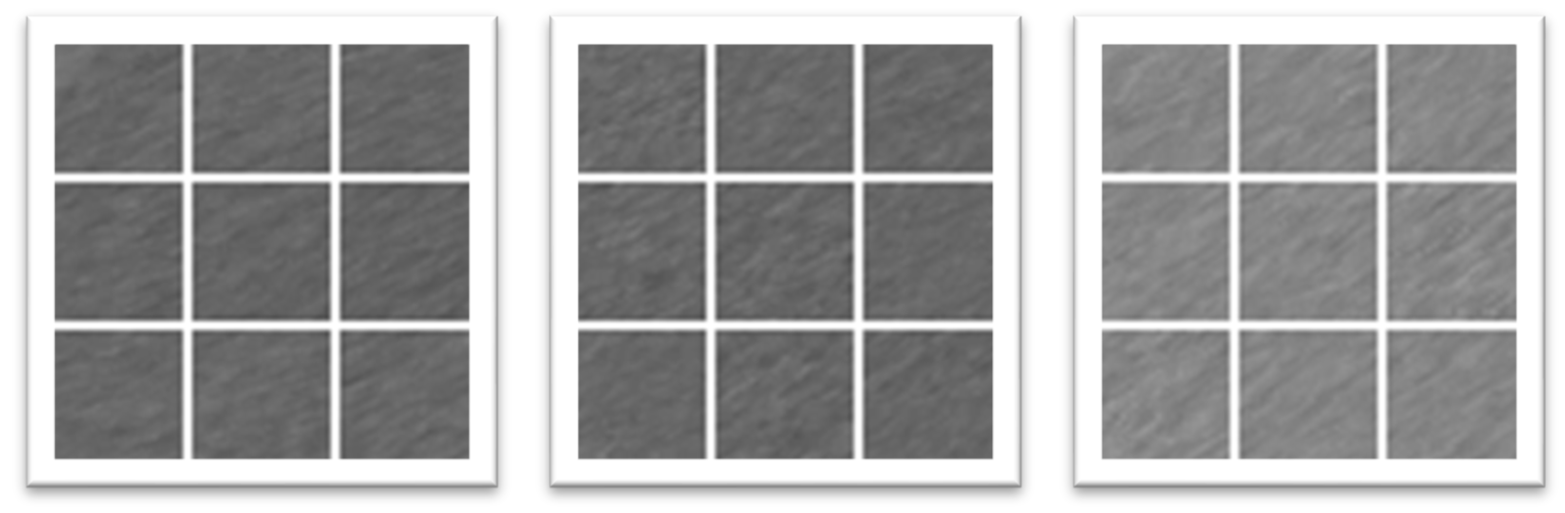
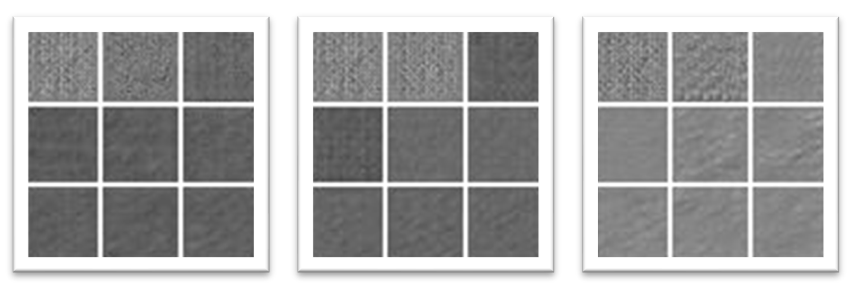
As shown in
Figure 4, with the increase in the number of epochs, the generated images gradually evolved from abstract to more concrete. From the final selected results, random samples show that it is indistinguishable to the naked eye whether the images were generated by the generator or not. Moreover, the grayscale co-occurrence matrix features of the generated images were highly similar to those of the original images. These observations demonstrate the effectiveness of the improved DCGAN. By adding the generated data to the training set, the quantity and feature richness of the data were increased, thereby enhancing the final classification performance of the classifier.
As shown in the data in
Table 4, the traditional CNN methods achieved relatively good classification results, with the overall classification accuracy of the four networks exceeding 90%. Among them, VGG16 achieved the highest accuracy, reaching 95.75%. After training the network models on the augmented dataset, the classification accuracy of each model improved to a varying degree. Specifically, LeNet’s accuracy increased by 1.88%, AlexNet’s accuracy improved by 1.06%, GoogLeNet’s classification accuracy rose by 2.59%, and VGG16’s classification accuracy increased by 2.97%. In the recognition of rock-class images, when the VGG network model was trained on the original dataset, the classification accuracy was only 65.28%. However, after data augmentation, the classification accuracy for rock-class images increased significantly to 87.05%, a substantial improvement of 21.77%.
5. Conclusions
In this study, CNNs were applied for the seabed substrate classification of multi-beam backscatter data images. Through experimentation, the following conclusions were drawn:
The CNNs can achieve good results when trained on small-sample datasets, with accuracy rates exceeding 90%.
The DCGAN was used to learn the data distribution of the original dataset and generate new multi-beam backscatter grayscale images for data augmentation. After training the four classification models on the augmented dataset, the classification accuracy improved compared to the original dataset, with the largest improvement observed in the VGG network, which increased by 2.97%. In the recognition of rock-class images, when the VGG network was trained on the original dataset, the classification accuracy was only 65.28%. However, after data augmentation, the classification accuracy for rock-class images increased significantly to 87.05%, representing a substantial improvement of 21.77%.
The introduction of a de-normalization and anti-standardization module into the traditional DCGAN learning model was shown to improve the quality of the generated images, as observed through visual inspection and the gray level co-occurrence matrix method.
This data augmentation approach can also be applied to other data-scarce domains, such as seabed target recognition. However, this method has limitations, specifically that the quality of the generated data from the DCGAN is unstable, necessitating the use of visual inspection and gray level co-occurrence matrices for selection. In future research, we aim to design a more stable data generator with better performance. Additionally, super-resolution image reconstruction techniques can effectively address the low-resolution issues of sonar images, which will be a key focus of our future studies.


