Article

A Deep Learning Approach for Identifying Intentional AIS Signal Tampering in Maritime Trajectories

College of Electronic Engineering, National University of Defense Technology, Hefei 230031, China
*
Authors to whom correspondence should be addressed.
J. Mar. Sci. Eng. 2025, 13(4), 660; https://doi.org/10.3390/jmse13040660
Submission received: 8 March 2025 / Revised: 21 March 2025 / Accepted: 23 March 2025 / Published: 26 March 2025
(This article belongs to the Section Ocean Engineering)

Abstract

:
In the field of maritime safety research, ship behavior analysis is usually based on data provided by automatic identification systems (AISs). Prevailing studies predominantly focus on detecting the behaviors of vessels that may affect maritime safety, especially the abnormal disappearance of ship AIS signals, neglecting subsequent measures to trace these illegal ships. To fill this gap, we propose a deep learning model named multi-dimensional convolutional long short-term memory (MConLSTM) to tackle the challenge of recognizing ship trajectories in cases where AIS signals are intentionally altered. By employing a self-supervised approach, the model is trained using historical real-world data. Extensive experiments show that MConLSTM exhibits superior analytical capabilities when it comes to processing and analyzing AIS data. Notably, even in scenarios with scant training data, the model exhibits exceptional performance, with an average accuracy 22.74% higher than the general model. Finally, we validated the practical significance and feasibility of the proposed method by simulating real-world scenarios.

1. Introduction

Currently, maritime transport facilitates 90% of global trade, with its prominence continuing to escalate [1]. The rapid expansion of the global shipping industry has led to a surge in ship traffic, posing numerous safety and efficiency challenges. To effectively manage and monitor ships’ dynamic behavior, the automatic identification system (AIS) has progressively become indispensable. The AIS system broadcasts a ship’s dynamic, static, and navigation-related data in a standardized format [2], which is received by both other vessels and shore-based systems. AIS data not only furnish basic ship information like position, course, and speed but also encompass inter-ship communication data [3], facilitating easy collection and offering a robust dataset for analyzing ship behavior. AIS data have typical spatiotemporal characteristics. The ship’s position, speed, course, and other information change with time, which is usually closely related to the behavioral patterns and purposes of navigation. Nonetheless, AIS transmits hundreds of millions of messages globally daily [4], leading to inevitable noise generation within the data due to wireless transmission instabilities and other objective factors. Consequently, extracting valuable information from vast and intricate AIS data and utilizing it judiciously have always been huge challenges.
To evade maritime supervision, deliberately altering AIS signals is a common behavior of illegal ships, especially in areas where the AIS signal is completely absent, which stems from environmental factors. In addition, some illegal ships will turn off AIS signals and follow other ships, which can also lead to the occurrence of incomplete trajectories. For this issue, prevailing studies predominantly focus on detecting trajectories with abnormal interruption, neglecting subsequent measures to trace these illegal ships.
Given the complexity of AIS data, it is difficult to identify trajectories that have been deliberately tampered with through manual analysis [5]. In recent years, rapidly developing machine learning has become an important approach for analyzing AIS data. In the actual process of maritime travel, ships with similar objectives tend to exhibit roughly similar trajectories, which can not only conserve fuel but also enhance navigation safety. Therefore, the historical trajectories of ships in an area inevitably correlate with the current behavior of ships, which provides a data foundation for machine learning methods to solve trajectory recognition.
To fill the gap in research, this paper proposes a deep learning approach to identify the subsequent trajectory of ships that tamper with AIS signals. Specifically, we transformed the issue into a classification problem through analysis. Subsequently, we designed a deep learning model, termed MConLSTM, that is capable of fully capturing the global and temporal characteristics of AIS data. Finally, we employed a self-supervised learning approach to train the deep learning model to address this classification problem.

2. Literature Review

Currently, the primary research focus on AIS data analysis lies in identifying and predicting abnormal ship behavior. In addition, there are also some other research points, such as the analysis of ship berthing. Fang and Yin [6] analyzed the behavior characteristics of ships berthing ashore using AIS data and established an evaluation model. Their focus is on designing evaluation indicators based on ships’ berthing behavior and conducting objective evaluations. Traditional machine learning and deep learning are increasingly pivotal in ship behavior analysis and anomaly detection [7].

2.1. Traditional Machine Learning in Maritime Supervision

Based on the existing analysis, traditional machine learning methods in maritime supervision can be categorized into two main types: probability-based models and clustering methods.
Probability models are fundamental for analyzing ship behavior, particularly when based on historical AIS data. These methods typically assume that ship behavior follows certain probability distributions and employ statistical learning to detect anomalies or predict future behavior. Dalsnes et al. [8] proposed a data-driven approach to predict vessel positions. The predictions are represented as Gaussian mixture models (GMMs), which provide a measure of uncertainty and can handle multimodality in vessel trajectories. A nearest neighbor algorithm was applied to two different data structures, and the accuracy and covariance consistency of both structures were tested on real data. This method was particularly useful for collision avoidance systems in autonomous surface vessels (ASVs). Mascaro et al. [9] explored anomaly detection using data-mined Bayesian networks learned from real-world AIS data and supplementary data. They developed both dynamic and static Bayesian network models, which are easy to examine and verify despite incorporating a large number of variables. The combination of dynamic and static modeling approaches improves the coverage of the overall model, thereby enhancing anomaly detection performance. However, the static components of the model might lack adaptability to rapidly changing maritime conditions, and the reliance on supplementary data could introduce complexity or potential biases. Zhou et al. [10] employed hierarchical timed colored Petri nets (HTCPN) and Markov chains to evaluate the emergency response process to ship fires. By modeling the ship fire emergency response process and calculating performance metrics using Markov chains, they provided targeted suggestions for optimizing emergency response capabilities. But, the static nature of Markov chains might not fully capture the dynamic and uncertain aspects of real-world emergencies. Validating the model in diverse scenarios could strengthen its robustness and applicability. Fridman et al. [11] presented an algorithm for selecting the best satellite observation window to detect moving vessels. Their model predicted vessel behavior within a time frame of 1–24 h and is integrated into the KINGFISHER maritime intelligence system for tracking suspected vessels with satellite sensors. This approach demonstrated the importance of probabilistic modeling in large-scale maritime surveillance.
Clustering methods are widely used in maritime supervision to group ship trajectories and detect abnormal behavior while being highly interpretable and applicable to a wide range of scenarios. Kumar and Ramanarayanan et al. [12] proposed a machine learning scheme based on HDBSCAN+ to identify abnormal ship behavior through clustering. By automatically adjusting clustering parameters based on the dataset, this method adapts to various scenarios and successfully detects maritime accidents reported by the Indian Ocean Regional Information Fusion Center (IFC-IOR). While the approach is innovative, its sensitivity to data density variations could be a drawback, and further research could focus on improving its robustness in heterogeneous datasets. Liu et al. [13] presented a hybrid clustering model for the probabilistic characterization of ship traffic and anomaly detection. First, ship trajectory characteristics are constructed based on static and dynamic features, and dissimilarities between trajectories are calculated using the Hausdorff algorithm. K-means is used to cluster trajectories based on departure and destination characteristics, while DBSCAN is applied to further refine the clustering within sub-trajectories. This hybrid approach was tested in Zhanjiang Port, demonstrating its effectiveness in detecting anomalies in ships. However, trajectory features extracted based on fixed rules may limit the effectiveness of anomaly detection, making the method of feature extraction a further research direction to improve model performance.
Additionally, machine learning has a wide range of application scenarios. To prevent ship-infrastructure collisions and ensure transportation safety, Komol et al. [14] represented an emergency clash avoidance control system. They also developed a simulation platform for movable bridge maritime and dynamic traffic management, which can effectively improve transportation strategies and reduce collision risks. Maelic et al. [15] proposed a method for recognizing false AIS signals by incorporating time division multiple access (TDMA) and employing the Kalman filter. They only analyzed AIS signals from the perspective of signals without considering the valuable behavioral information contained in AIS signals, which was not the focus of current research. Bloisi [16] combined different data to achieve ship monitoring, including AIS data and video data, which enabled effective monitoring of ship behavior in areas where radar was not available. This multimodal approach was promising, but challenges related to data synchronization and processing efficiency need to be addressed in future work to improve its scalability and practicality.
It is noteworthy that Kutluyil [17] conducted a comprehensive review of the application of machine learning in AIS data processing. In addition, he pointed out the powerful ability of artificial intelligence to analyze AIS data and elaborate on future development trends in areas such as ship behavior pattern recognition and target classification. However, with the increasing amount of data and more complex regulatory requirements, modern maritime supervision is gradually developing towards multi-source data fusion, intelligence, automation, and multi-task systems. Traditional machine learning methods are more suitable for single tasks based on simple data due to their limitations. Daneshfar [18] indicated that deep learning is highly effective in extracting features from nonlinear and complex data, which will play an important role in current and even future research.

2.2. Deep Learning Methods Based on AIS Data

Supervised learning is the most widely used method in deep learning, and it is especially suitable for mining features from complex nonlinear data. In the application of deep learning in maritime vessel supervision, existing research can be broadly categorized into two areas: vessel behavior analysis and anomaly detection and vessel trajectory prediction and risk assessment.
Deep learning has been widely adopted in vessel behavior analysis and anomaly detection, particularly for handling complex nonlinear data. Liu et al. [19] proposed a monitoring and detection mechanism for vessel abnormal behavior based on a graph attention prediction and Reconstruction Network. This mechanism effectively captures the interdependencies among vessel behavior characteristics, demonstrating the potential of graph-based approaches in modeling complex relationships within maritime data. By introducing advanced deep learning techniques, their approach not only improves detection accuracy but also enriches the methods for identifying abnormal vessel behaviors. However, the reliance on graph structures may increase computational complexity, particularly when applied to large-scale AIS datasets, which could pose challenges for real-time applications. Duong et al. [20] designed a new encoding method (four-hot vector) based on one-hot encoding, which is different from the 4D real-valued vector [21,22,23] that is commonly used. This encoding method is more conducive to learning the spatial and temporal characteristics of AIS data. Subsequently, they exploited state-of-the-art neural network schemes to learn a probabilistic representation of AIS tracks and a contrario detection to detect abnormal events.
Integrating multiple tasks into a unified system has become a research hotspot, allowing for more efficient and comprehensive maritime data analysis. Duong and Rodolphe [24] developed a multitasking and universal deep learning framework based on a variational recurrent neural network (VRNN). This framework could simultaneously handle tasks such as trajectory reconstruction, abnormal behavior detection, and track type recognition, showcasing the versatility of VRNNs in maritime applications. Their method embedded AIS data into a new representation space, effectively addressing noise and sampling issues in AIS data. Nevertheless, the projection might lead to the loss of important information in AIS data, which was an unavoidable problem.
Despite the significant role of deep learning in vessel anomaly detection, certain limitations remain. Pierre and Arnaud [25] designed a deep learning model centered on the transformer architecture, which can effectively identify illegal vessels that deliberately disable their AIS signals. This highlights the potential of attention mechanisms in capturing long-range dependencies in AIS data. Similarly, Song [26] and Ma [27] implemented anomalous trajectory detection using recurrent neural networks (RNNs) [28], achieving high accuracy on manually annotated datasets. However, the reliance on manual annotation, often based on specific thresholds, may introduce bias and limit the adaptability of these methods to diverse real-world scenarios. Additionally, the interpretability of deep learning models in explaining detected anomalies remains a challenge, which is crucial for gaining the trust of maritime operators and regulators.
In the domain of vessel trajectory prediction and risk assessment, deep learning has also made significant strides. Gao and Zhu et al. [29] developed a model for predicting collision risks among vessels in a given region. Their approach employed clustering techniques on raw AIS data to preliminarily identify vessels at potential risk, significantly reducing the volume of data to be processed. Subsequently, a deep learning framework was utilized for maritime risk assessment. While this two-step approach enhanced computational efficiency, the accuracy of the clustering stage might influence the overall performance, and the method’s sensitivity to varying traffic densities warrants further investigation.
Xiao et al. [30] proposed a bidirectional data-driven trajectory prediction method based on deep learning. By reversing trajectory data, their approach could more comprehensively capture implicit information in AIS data, enabling accurate predictions of vessel behavior. This innovative use of bidirectional learning demonstrated the potential for improving prediction robustness. Similarly, Kim [31] designed a layered neural network to predict vessel behavior in port areas, extracting trajectory features from different perspectives using specialized deep learning modules. While these methods showcased the power of deep learning in feature extraction, their performance in highly dynamic environments, such as congested ports or regions with unpredictable traffic patterns, may require further validation.
In summary, deep learning has been extensively applied in maritime vessel supervision, particularly in vessel behavior analysis, anomaly detection, trajectory prediction, and risk assessment. While deep learning has demonstrated remarkable performance in these tasks, challenges such as reliance on large datasets and potential labeling biases remain. Future research should focus on optimizing deep learning models and training methods to enhance their robustness and accuracy in practical applications. This paper addresses the challenge of identifying the subsequent trajectories of ships intentionally tampering with AIS signals, a task that is difficult to achieve using unsupervised methods like those in [32,33,34]. To mitigate the bias introduced by manual annotation, self-supervised learning can be employed to automatically extract supervised information from unlabeled datasets, offering a promising solution for model training.

3. Method Overview

As depicted in Figure 1, this paper employs self-supervised learning to construct the training dataset from raw AIS data. Then, we design a deep learning model, MConLSTM, based on the characteristics of AIS data. This model accepts two trajectories as inputs and outputs the probability that two trajectories come from the same voyage.

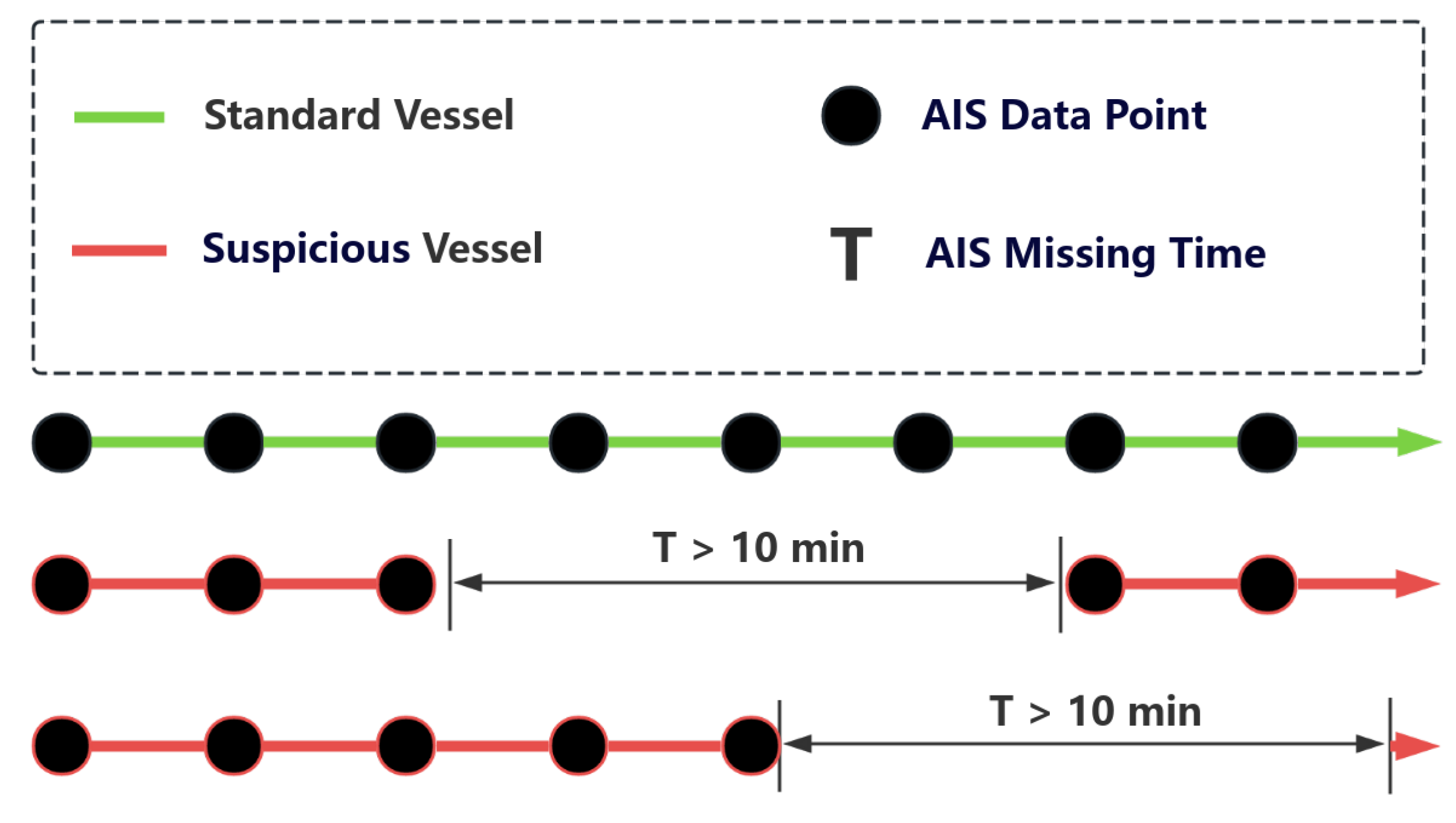
3.1. Data Processing

In order to accurately reflect the behavior status of ships while minimizing the amount of data, it is necessary to sample and filter AIS data. The data utilized in this paper originate from historical real track segments, and some examples are depicted in Figure 2. Given that the interval of the original AIS signal typically ranges between 3 and 10 s, and considering the relatively slow navigation speed of ships, such dense AIS data are unnecessary for describing ship behavior. Therefore, we filter out duplicate points from the original data and sample the ship’s trajectory at 10 min intervals.
Given the above, AIS data encompass various types of information, such as latitude, longitude, ship speed, the direction of travel, maritime mobile service identity (MMSI), dynamic and static information, as well as other attributes reflecting behavioral states. This paper only focuses on the attributes in AIS data that are directly related to the behavior status of ships while disregarding information pertaining to the ship’s identity and behavior. To enhance understanding of the data and improve model performance, certain features are expanded upon based on the existing AIS data, as discussed in Equation (1).
m i = l o n i , l a t i , s p e e d i , h e a d i , t i m e i .
In Equation (1), m i is the processed AIS data of a ship at a certain time, [ l o n , l a t ] is the longitude and latitude of the trajectory point, s p e e d is the running speed of the ship, and h e a d is the direction of travel of the ship, namely the angle between the heading and geomagnetic north. Continuous trajectory points m i form a complete trajectory [ m 1 , m 2 , ] , representing a multidimensional time series.

3.2. Dataset Construction

As depicted in Figure 3, complete tracks are randomly selected from two different ships. Tracks with a duration of one hour are chosen. However, data where the time interval between two tracks is excessively long or the distance between them is too great are evidently unsuitable for training purposes. Thus, the selected tracks must adhere to the following criteria: the time interval between the end of the preceding track and the commencement of the subsequent track should be under one hour, and the distance between them should not exceed d m a x ( d m a x represents the maximum distance a ship can traverse within an hour). Subsequently, these two tracks are concatenated. This procedure is repeated iteratively to generate 1 million datasets.
To ensure the balance of training data, a large amount of opposite training data is also essential, and the subsequent operations are performed continuously, as illustrated in Figure 4. Initially, a complete track is randomly chosen from all ship trajectories, followed by the random selection of two segments with an interval not exceeding one hour. This one-hour interval between the segments is necessitated by the time taken for the vessel to update AIS data. Subsequently, these two trajectories are combined to obtain a training set representing a normal ship. By repeating the above operations, the same number of opposite training sets will be generated.
Here, we have converted the original problem into a binary classification problem and preliminarily processed the AIS data into a training dataset for deep learning. The subsequent section will involve conducting final preprocessing based on the extracted feature data, designing a model tailored to the dataset, and strategically utilizing the dataset for model training.

3.3. Model Design

Due to the complexity of AIS data, it is imperative for the deep learning model to capture the inherent time-series characteristics within the AIS data overall. As shown in Figure 5, we develop a deep learning model called MConLSTM using a convolutional neural network (CNN) [35] and long short-term memory (LSTM) [36], which consists of three parts: separation and processing of attributes, data importance analysis, and temporal feature extraction.

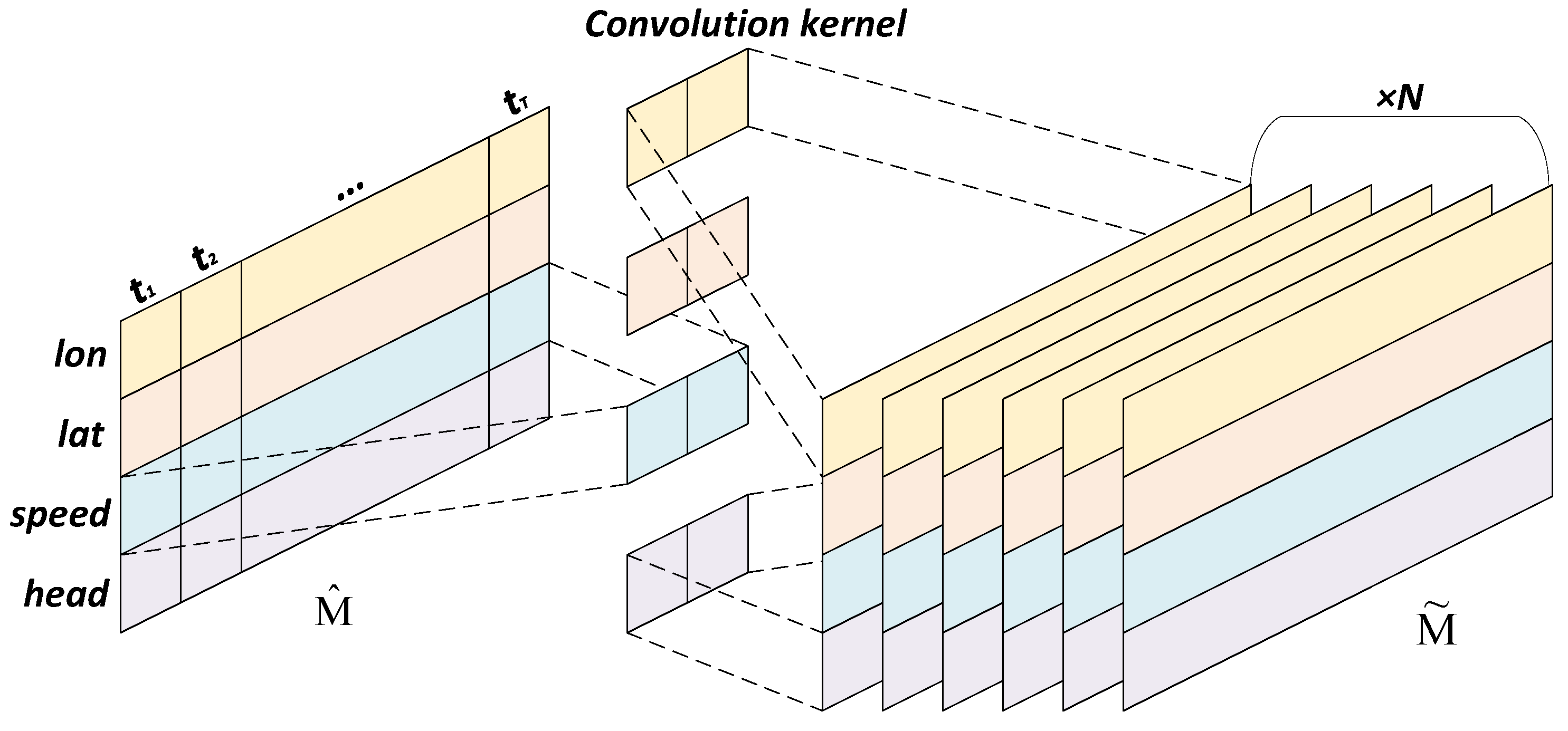
3.3.1. Separation and Processing of Attributes

To ensure that the training data include the behavioral characteristics of all ships and be as concise as possible, we opted to isolate four attributes from AIS data, including l o n , l a t , h e a d , and s p e e d . Considering that the interval of AIS data has been sampled as a fixed value, t i m e is not necessary for training. Consequently, the training data is determined as temporal data with four attributes, which are then segregated into four individual temporal data by attributes. Trajectory M = [ m 1 , m 2 , , m T ] containing T AIS data points is processed as lon , lat , speed , head , where lon is [ l o n i ] , i { 1 , 2 , , T } , lat is [ l a t i ] , i { 1 , 2 , , T } , speed is [ s p e e d i ] , i { 1 , 2 , , T } , and head is [ h e a d i ] , i { 1 , 2 , , T } .
Given the potential variance in measurement scales across different attributes, directly inputting AIS data into the model may result in several challenges, including overfitting, gradient instability, and convergence issues, which can diminish training efficiency and accuracy. Consequently, data normalization is also essential before training, which ensures that all features are adjusted to similar scales. In addition, the normalization methods of different attributes should also be different. Due to the fixed upper and lower limits of longitude and latitude and our objective of enabling the model to acquire geographical knowledge through these coordinates, we normalize l a t and l o n using Equation (2). However, the behavior of ships in different trajectories varies greatly and is obviously affected by the geographical environment. Hence, we employ Equation (3) to normalize s p e e d and h e a d , which is shown as follows:
N l ( x ) = x 180 ,
N c x = x x m i n x m a x x m i n ,
where x m i n is the minimum value of x , and x m a x is the maximum value of x . Subsequently, we obtained the input for the deep learning model:
Input = lon ^ = N l ( lon ) lat ^ = N l ( lat ) speed ^ = N c ( speed ) head ^ = N c ( head ) .

3.3.2. Data Importance Analysis

In order to learn the features of trajectories more accurately, we need to conduct data importance analysis. AIS data are high-dimensional temporal data containing numerous noise points and missing values. In addition, the importance of data from different positions in our task varies within the entire trajectory. If we focus solely on the temporal characteristics of AIS data, the substantial extraneous data within the trajectory may prevent the model from effectively capturing long-term dependencies. Therefore, we need a module to judge the importance of data in the trajectory.
In recent years, CNN has been primarily employed in the field of computer vision, which excels in capturing local features of data with the unique sliding mechanism. Furthermore, it can achieve a broad global perspective through deep structures. Since trajectories have a similar data format to images, we can employ CNN to obtain the importance of local data in a trajectory. Moreover, with its powerful feature extraction ability, CNN can learn these complex spatial features from AIS data preliminarily.
Since image data are not time-series, researchers typically use a convolution kernel for the entire matrix. However, due to the varying influences of different attributes on behavior analysis, different attributes may require different parameters to make the deep model converge during the optimization of deep learning model parameters for AIS data. To independently calculate the importance of each position in different attributes, we design a multidimensional convolution network (M-CNN).
As illustrated in Figure 6, independent convolution kernels are employed to calculate the importance of various attributes in AIS data. Through M-CNN, we can obtain the trajectory M ˜ that contains the importance of data as follows:
M ˜ = M-CNN ( M ^ ) ,
where M ^ R 4 × T is [ lon ^ , lat ^ , speed ^ , head ^ ] T , which we have obtained in the previous section. Specifically, we employ different one-dimensional convolution kernels to determine the importance of different positions in lon ^ , lat ^ , speed ^ , head ^ R T :
τ = Con 1 D ( X , K , N ) | X M ^ ,
M ˜ = Reshape ( τ ) ,
where Con 1 D ( X , K , N ) represents performing one-dimensional convolution on X using a K-dimensional convolution kernel with N channels while keeping the length of the trajectory data T unchanged. τ R 4 × N × T denotes the result of the convolution operation, and τ is then reshaped into a two-dimensional matrix M ˜ R T × H for the subsequent extraction of temporal features. Compared to the original trajectory M , important data in the trajectory are automatically enhanced, while unimportant data are weakened. In addition, the dimensionality H = 4 × N of each data point in M ˜ is higher than that in M , which is more conducive to the subsequent feature reduction, like word vector embedding in natural language processing (NIP).

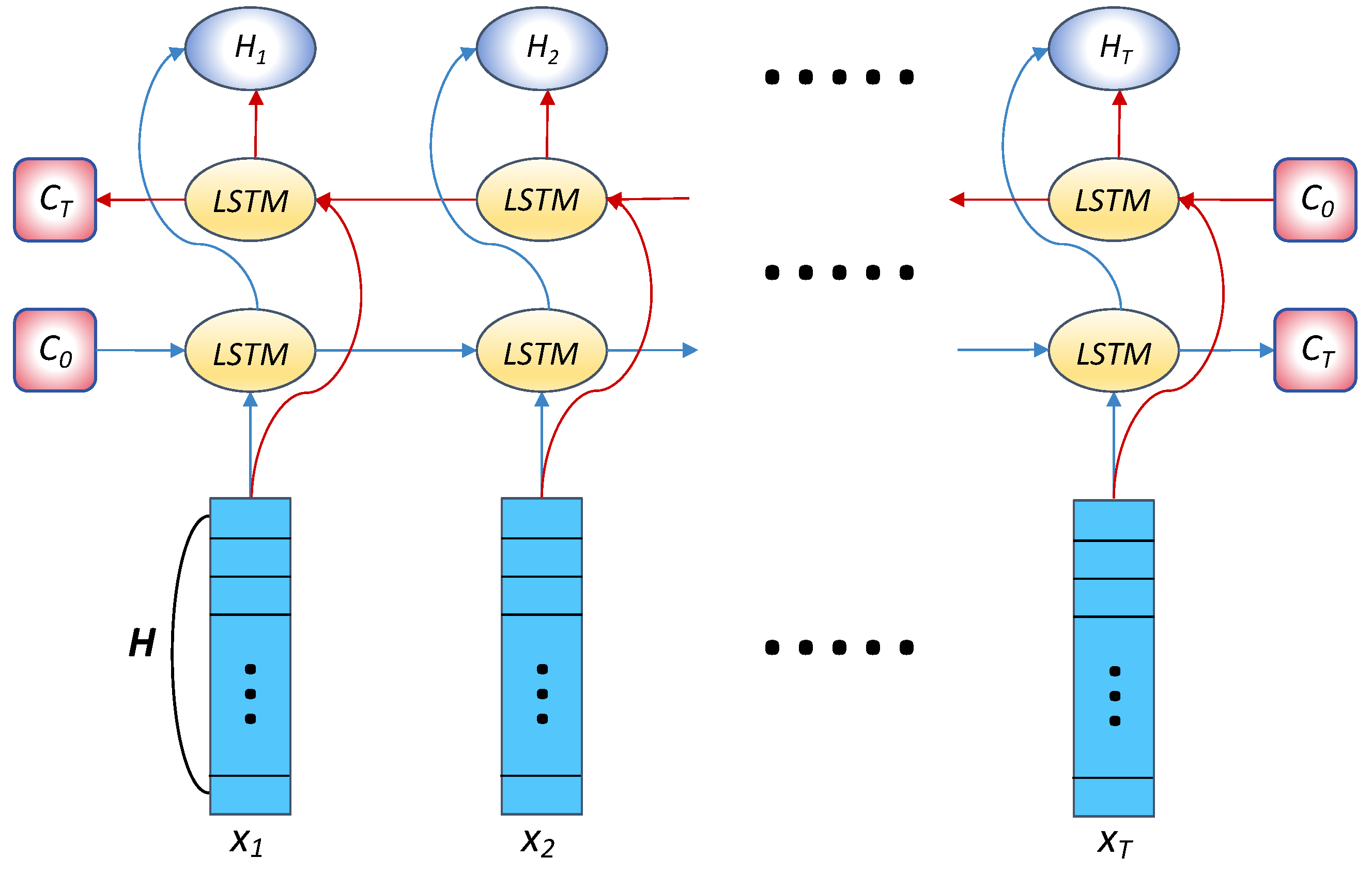
3.3.3. Temporal Feature Extraction

However, relying solely on a CNN is insufficient to comprehensively capture the characteristics of AIS data. The temporal dependency within AIS data is also crucial. The navigational status of a vessel depends not only on its current position but also closely on its previous navigation history. The RNN and transformer [37] exhibit superior performance in learning from time series data. When designing a model for complex and large-scale AIS data, the considerations of both the model’s performance and the consumption of training resources are imperative while avoiding overfitting as much as possible.
On the other hand, RNNs have evolved into variants such as LSTM, which typically demonstrate outstanding performance in processing sequential data due to their unique gating mechanisms, including input gates, forget gates, and output gates, effectively alleviating the common issues of gradient vanishing and exploding encountered in a traditional RNN. Therefore, we chose LSTM with lower resource consumption to extract temporal features.
For the trajectory M ˜ R T × H that contains the importance of data from different locations, we utilize a bidirectional LSTM architecture to extract temporal features as Figure 7. A bidirectional LSTM incorporates two parallel LSTM layers, with its primary advantage being the capability to capture bidirectional information in time series data. This advantage allows bidirectional LSTM with the hidden size λ to extract richer features in long sequence analysis as follows:
H T = Bi-LSTM ( M ˜ ) = h T + h T ,
where Bi-LSTM ( · ) represents the overall function of the bidirectional LSTM for processing M ˜ , H T R T × λ is the temporal features of M ˜ , and h T + R T × λ and h T R T × λ are the outputs of two LSTM layers:
h T + = LSTM + ( M ˜ ) = [ h 1 + , h 2 + , , h T + ] ,
h T = LSTM ( M ˜ ) = [ h 1 , h 2 , , h T ] ,
where h t R λ , t { 1 , 2 , , T } represents the output state of the t th time step of an LSTM layer. In addition, h t + and h t are not essentially different but only process M ˜ in different directions. The computation process for the t th input x t is as follows:
i t = σ ( W i x x t + W i h h t 1 + b i ) ,
f t = σ ( W f x x t + W f h h t 1 + b f ) ,
C ˜ t = tanh ( W c x x t + W c h h t 1 + b c ) ,
C t = f t C t 1 + i t C ˜ t ,
o t = σ ( W o x x t + W o h h t 1 + b o ) ,
h t = o t tanh ( C t ) ,
where C t is the cell state at time step t, i t and f t , respectively, represent the input gate and forget gate, with o t as the output gate, and tanh ( · ) is the hyperbolic tangent function.
After T time series points of M ˜ have been entirely inputted, the extracted temporal features H T will be concatenated with M ˜ , with the computation steps as follows:
ξ = Concat ( H T , M ˜ ) .
Subsequently, ξ is reshaped into a one-dimensional vector containing global information and temporal features of the trajectory M . Finally, a multilayer perceptron (MLP) layer with S i g m o i d ( · ) as an activation function is applied to obtain the probability P that the subsequent trajectory is generated by the same ship.
P = Sigmoid ( MLP ( ξ ) ) .
To measure the possibility of two trajectories being generated by the same voyage, we completed the design of MConLSTM, which can effectively handle large-scale and high-dimensional AIS data. In comparison to the traditional model, MConLSTM has the capability to autonomously acquire the spatiotemporal characteristics of AIS data from individual attributes. Specifically, M-CNN ensures a global perspective of the model to prevent it from converging to local optimal solutions, and bidirectional LSTM ensures the extraction of temporal characteristics from AIS data. Additionally, the model’s depth is primarily reflected in the deep convolution layer, with the convolutional layer containing significantly fewer parameters than LSTM and transformer, thereby reducing the computational resources needed for training.

4. Result Evaluation

In this chapter, we will utilize the constructed dataset to train the proposed model. Following the introduction of the experimental environment and the configuration of key parameters, our attention will shift towards analyzing the experimental results. Through a series of comparisons, we aim to evaluate the effectiveness of the model. Subsequently, we will provide a comprehensive summary of this paper, identifying its limitations and suggesting avenues for future research and prospects.

4.1. Training Environment

When training the model designed in this experiment, the parameters are set as shown in Table 1. In addition, two callback functions are also employed, one for automatically adjusting the learning rate and the other for saving the optimal model.
The dataset constructed in the preceding section comprises two opposite datasets containing a total of 2 million training data items. To evaluate the performance of MConLSTM and ensure its generalization capability, three-quarters of the whole training data are randomly allocated to the training set, with the remaining data designated for the test set. The computations are executed on the NVIDIA GeForce RTX 4070 Ti and the 13th Generation Intel (R) Core (TM) i7-13700KF processor operating at 3.40 GHz. Each iteration requires approximately one min to execute and continually monitors and records changes in the loss function and accuracy metrics. Subsequently, the optimal model achieved during the training phase is preserved.

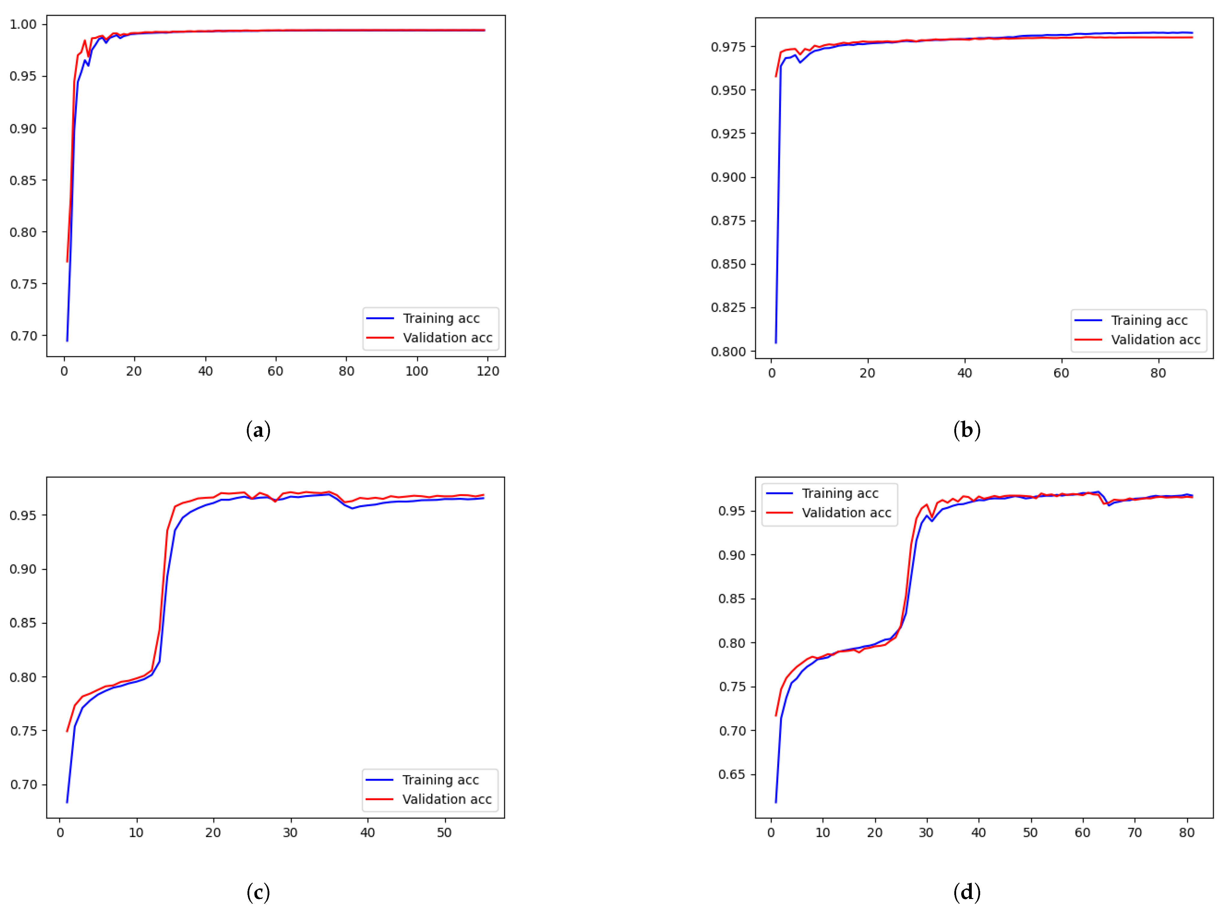
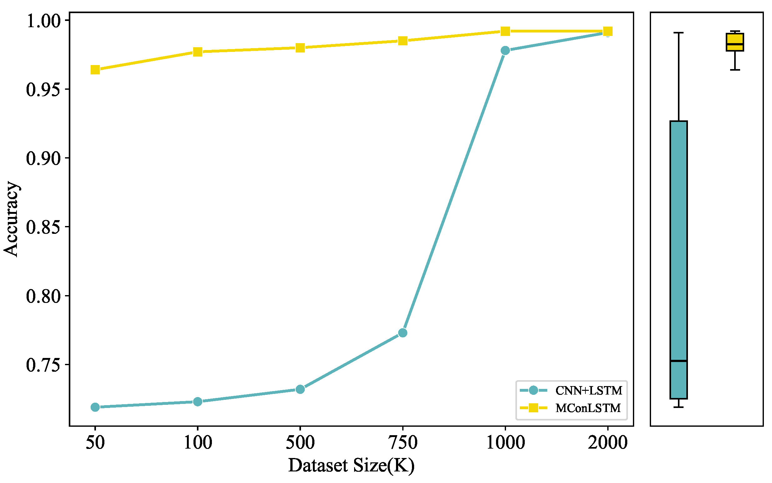
4.2. Training Results

There are two types of errors that may occur during the experiment: one is identifying the trajectory of the same ship as generated by two ships, and the other is mistaking the trajectory generated by two ships as that generated by one ship. From the analysis of Table 2, when testing with two completely opposite datasets, the recognition accuracy of both datasets can reach almost 99%. Firstly, the effectiveness of the model on AIS data is demonstrated. This confirms that the model trained on the dataset exhibits excellent generalization, and the trajectory recognition of the target sea area holds universal value. Figure 8 demonstrates the entire process of MConLSTM training, and it is evident that the accuracy of MConLSTM is very close to the optimal value after 40 iterations without obvious overfitting.

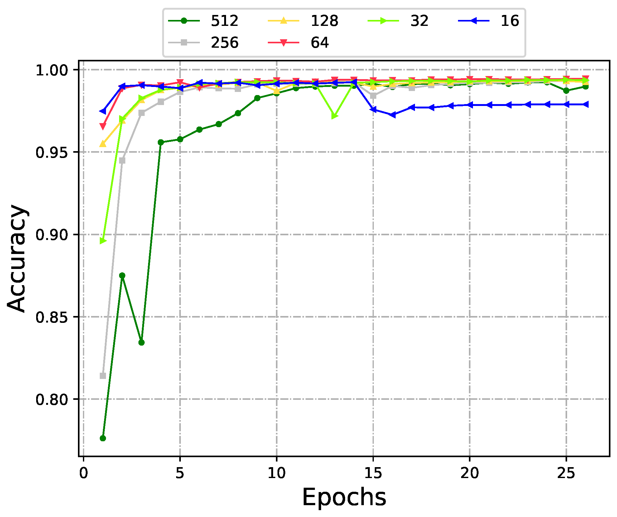
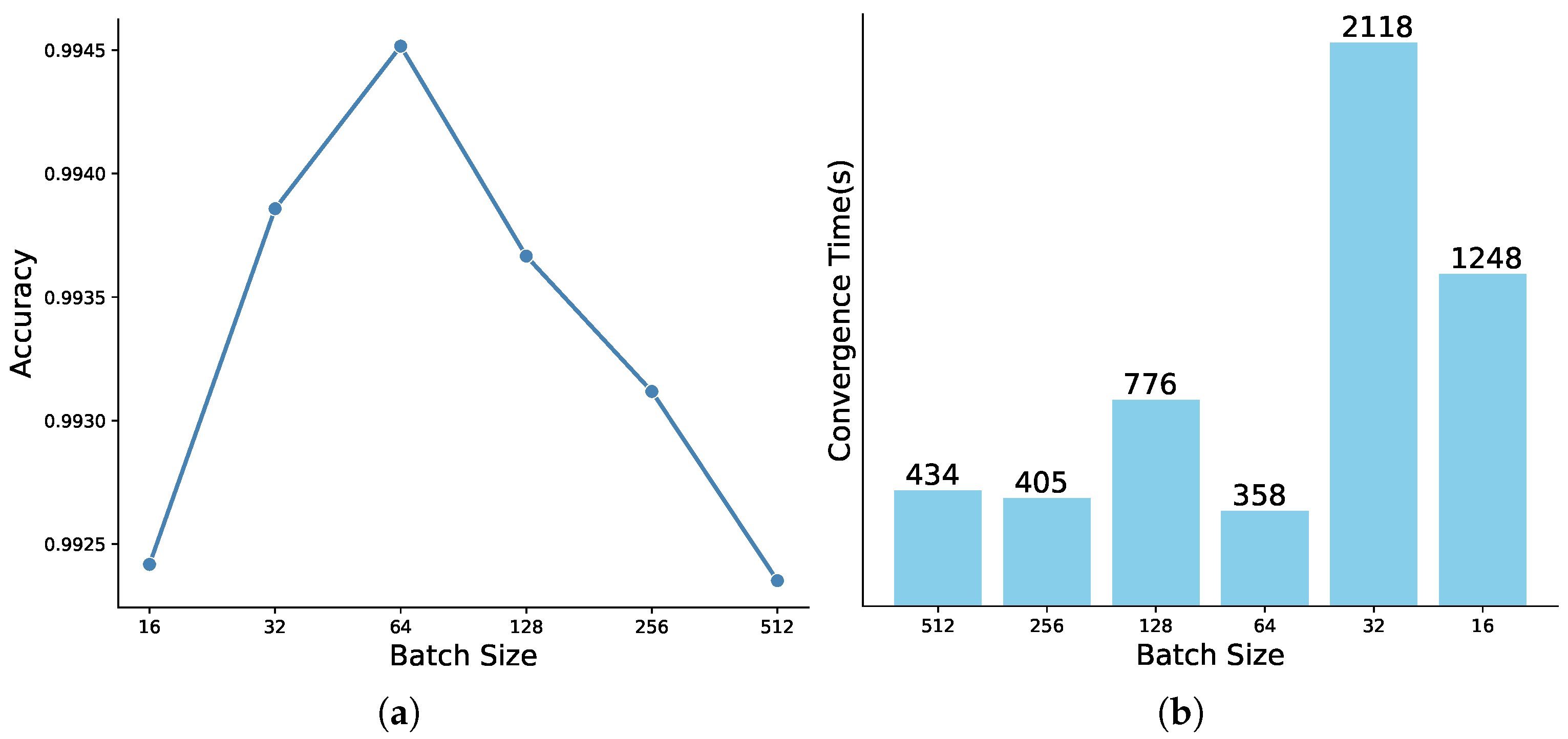
4.3. Hyperparameter Optimization

Among all hyperparameters used in this paper, L e a r n i n g R a t e is automatically attenuated, and the O p t i m i z e r and L o s s F u n c t i o n are selected according to the binary classification problem. These hyperparameters do not need to be optimized. For the depth of our model, it varies with the complexity of the problem to be solved. Therefore, against the background of this paper, we only need to optimize the value of batch size. We experimented with varying batch sizes ranging from 512, progressively halving it down to 16, and the training results of the model under different batch sizes are shown in Figure 9. Interestingly, we observed that a batch size of 64 yielded the optimal results, achieving the highest accuracy as well as the shortest convergence time.
The reason behind this phenomenon lies in the balance achieved with a batch size of 64. Smaller batch sizes, such as 16, mean more noise in the gradient updates due to the higher variance in the data distribution within each batch. This noise can hinder the model’s ability to converge to the optimal solution. On the other hand, larger batch sizes, such as 512, reduce the noise but may compromise the model’s generalization capability by averaging over a larger portion of the training data, potentially overlooking local details.
A batch size of 64 strikes a balance between these two extremes. It reduces the noise in the gradient updates compared to smaller batch sizes, allowing the model to converge more smoothly. At the same time, it still captures enough local details from the data to maintain good generalization, enabling the model to achieve a higher accuracy. Additionally, a moderate batch size often leads to improved computational efficiency, resulting in a shorter convergence time.
Naturally, it can be found that there are obvious differences in training with different batch sizes. Figure 10 further shows the impact of different batch sizes on model training. We can easily find that when the value of batch size is 64, the model not only obtains the highest accuracy but also spends the least training time. Smaller batch sizes (e.g., 16 or 32) introduce more noise in gradient updates due to higher variance, which can hinder convergence, while larger batch sizes (e.g., 128 or 256) may lead to smoother but less frequent updates, potentially causing the model to converge to suboptimal solutions. Additionally, a batch size of 64 aligns well with the hardware’s parallel processing capabilities, reducing training time without compromising accuracy.

4.4. Ablation Study

As shown in Figure 11, the parameters of MConLSTM are much smaller than transformer and LSTM, which represents less computational resource consumption and training time. This is also an important reason why we gave up using transformer. First of all, the complexity of the model should be analyzed. This paper compares several models commonly used to process series data. Among them, MLP is essential for almost all deep learning models. We ensure that the parameters of each model are as similar as possible, such as the number of channels of LSTM and CNN and the dimension of MLP. Considering the above, MConLSTM has a similar number of parameters as MLP, and then we will evaluate its capability to analyze AIS data.
To demonstrate the adaptability of our design model to the AIS dataset more clearly, this paper conducts a series of comparative experiments. Firstly, keeping the size of the test dataset and model constant, we varied only the size of the training dataset to observe its impact on the training results of MConLSTM. The performance of our model as the training dataset size decreases is shown in Figure 12. It is evident that as the size of the training dataset decreases, the accuracy of the model hardly decreases, all above 95%, and there is no obvious overfitting phenomenon. On the one hand, convergence problems caused by more complex training data may explain the sudden drop in accuracy after stabilization during training. Since the dataset is randomly constructed, it is impossible to avoid such a problem. However, we can solve it by preserving the optimal model. On the other hand, the training curves exhibit a staircase pattern in some portions due to the insufficient initial learning rate that prevented the model from further convergence. Accuracy can continue to rise only after the learning rate decays, which increases convergence epochs.
Moreover, another comparative experiment was conducted to demonstrate the advantages of MConLSTM in learning AIS data features compared to traditional and widely used architectures. Specifically, we compare the accuracy of MConLSTM and multiple models based on CNN, LSTM, and transformer during the training process. Due to the fact that the transformer is not directly suitable for processing AIS data, we chose its two variants, CNN+Transformer(CMT) [39] and Bi-LSTM+Transformer [40], for experimentation.
The experiments were carried out using the same dataset, ensuring that all models were trained under identical conditions and with equivalent depths to ensure a fair comparison. As shown in Figure 13, the results revealed that MConLSTM achieved the highest accuracy on the test set, surpassing the performance of other models. Furthermore, MConLSTM exhibited the fastest convergence speed during training, indicating its efficiency in learning the underlying patterns and features from the AIS data. Evidently, MConLSTM not only excels in capturing spatial features and local correlations in data but also incorporates the ability to analyze and process sequential data.
In fact, the number of anomalous behaviors is relatively small compared to the vast total amount of AIS data. Therefore, to verify the performance of our model in the absence of sufficient training data, we also conduct comparative experiments. Specifically, we compare MConLSTM with CNN + LSTM, which directly uses trajectories as input and has the same depth as MConLSTM. As we can see, the performance of the two models under different sizes of training datasets is shown in Figure 14. As the training dataset size decreases continuously, the performance of the CNN + LSTM model declines significantly. When the training dataset is small, the average accuracy of MConLSTM is 22.74% higher than that of CNN + LSTM. This shows that MConLSTM can still learn the characteristics of AIS data well even when data are scarce. Correspondingly, in reality, when there are fewer special cases, we cannot obtain a mass number of datasets for model training and then MConLSTM can still achieve excellent results. At the same time, MConLSTM can also give full play to its characteristics when dealing with other multidimensional time series data.

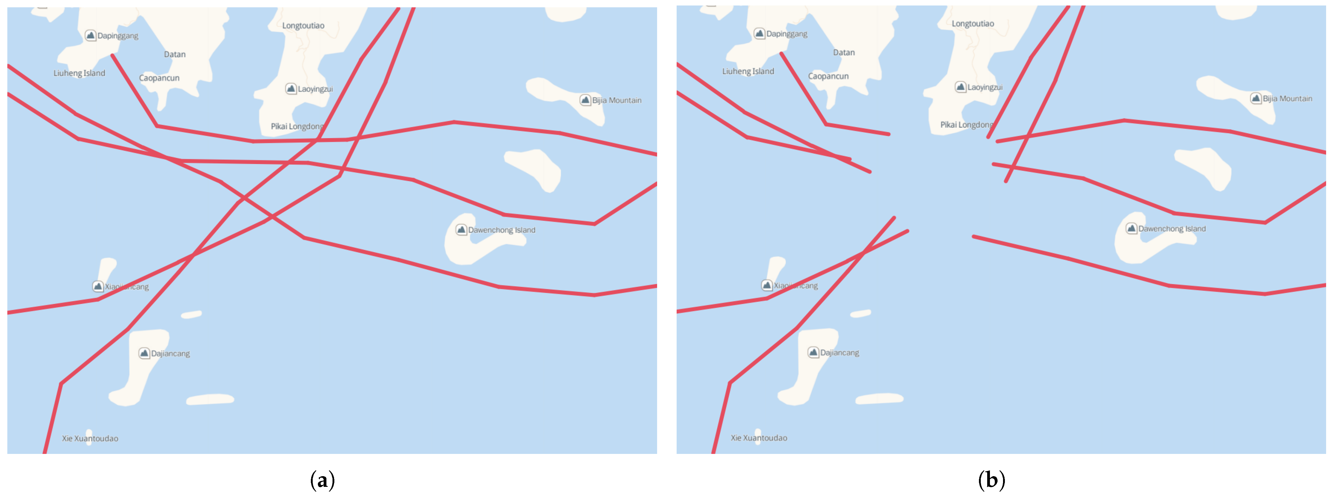
4.5. Case Study Simulation

Now, we begin to consider the practical application issues in the actual situation. On the sea, ships sailing normally and legally continuously broadcast their AIS signals. If a ship suddenly ceases to broadcast AIS signals, it is deemed suspicious. Considering various emergencies or objective effects, as illustrated in Figure 15, it is stipulated that a ship failing to broadcast AIS signals in non-breathable waters for over ten min is deemed suspicious. Subsequently, all possible subsequent tracks near the vanishing point within two hours, with the vanishing point as the center, are recorded. The front and rear tracks are then spliced and input into the model to the probability value of two tracks from the same ship. Eventually, the track with the highest probability is selected as the most likely new track of the ship.
To ensure the model’s effectiveness in practical applications, a specific area depicted in Figure 16a was selected for simulation experiments. As shown in Figure 16a, the area contained the trajectories of several ships over a certain period. If the whole AIS signal disappeared in a certain area in the center of Figure 16a, multiple abnormal tracks and possible subsequent tracks would be generated, as in Figure 16b. We selected a certain abnormal track and its possible subsequent tracks for analysis, as shown in Figure 16c. These potential trajectories were combined with the abnormal trajectory and input into the trained model after processing to obtain the matching probability for the front and rear trajectories, which were then annotated in Figure 16d. Subsequently, the probability of these possible follow-up trajectories was compared. The track with a maximum probability value was considered the most probable subsequent track. If all the results did not exceed 50%, then we had reason to think that the ship deliberately turned off its AIS signal and followed other legitimate ships. Among all potential subsequent trajectories in Figure 16d, the trajectories labeled as ➂ and ➃ met our matching criteria, with trajectory ➃ reaching a probability of 95.77%, the highest among all possible outcomes, surpassing 95%. Consequently, it was natural to conclude that trajectory ➃ was the most probable subsequent trajectory of the abnormal ship that we selected, followed by trajectory ➂. Then, we went back and observed Figure 16a for verification and found that trajectory ➃ was indeed the real follow-up trajectory of the vessel in Figure 16c.
In this section, we simulated the actual trajectory recognition scenario to describe the application process of our method in addressing practical challenges. The experimental results demonstrated the effectiveness of our method in solving practical problems. At the same time, it also reflects the practical significance of the method proposed in this paper.

5. Conclusions

To address the subsequent track identification challenge posed by intentional alterations to marine vessel identification information during navigation, this paper first conducted a detailed analysis of the issue. We then employed the self-supervision learning method to reframe the problem as a binary classification problem. Leveraging historical real AIS data to construct a labeled dataset, we developed a model (MConLSTM) to discern the characteristics of AIS data and solved this binary classification problem. The model demonstrated the mighty ability to process AIS data. Subsequently, a series of comparative experiments was designed to validate the model’s learning capabilities with AIS data. Our model achieves the highest recognition accuracy in this work, outperforming the models based on transformer. In particular, when faced with a small number of training datasets, MConLSTM achieved an average accuracy of 22.74% higher than CNN + LSTM. The final test, simulating real-world scenarios, demonstrated the efficacy of the method proposed in this paper for addressing real-world challenges.
However, there are still some issues here. Owing to diverse geographical conditions, ship densities, and climates across various sea regions worldwide, this paper only utilizes historical data from a specific sea area for training. Consequently, the trained model lacks global applicability. Nonetheless, the training of this model exhibits positive generalizability concerning AIS data. Expanding the scope of AIS data used for training will enhance the model’s universality. This paper does not address the scenario where illicit vessels deliberately disable AIS transmission and solely rely on visual navigation, as this would necessitate a substantial dataset of AIS records to analyze actual illicit vessel behavior accurately. This aspect could serve as a promising avenue for future research endeavors, contributing significantly to maritime safety.

Author Contributions

Conceptualization, R.J. and C.C.; Methodology, X.L.; Validation, X.L., R.J. and C.C.; Investigation, N.S. and T.W.; Writing—original draft, X.L.; Writing—review & editing, R.J., C.C. and N.S.; Project administration, R.J., C.C. and N.S.; Funding acquisition, R.J., C.C. and T.W. All authors have read and agreed to the published version of the manuscript.

Funding

This research received no external funding.

Data Availability Statement

The original contributions presented in this study are included in the article. Further inquiries can be directed to the corresponding authors.

Conflicts of Interest

The authors declare no conflicts of interest.

References

  1. Wan, Z.; Chen, J.; Makhloufi, A.E.; Sperling, D.; Chen, Y. Four routes to better maritime governance. Nature 2016, 540, 27–29. [Google Scholar] [CrossRef] [PubMed]
  2. International Maritime Organization (IMO). Revised Guidelines for the Onboard Operational Use of Ship-Borne Auto-Matric Identification Systems (AIS); Tech. Rep. Resolution A.1106(29); International Maritime Organization (IMO): London, UK, 2015. [Google Scholar]
  3. Rong, H.; Teixeira, A.P.; Guedes Soares, C.; Santos, T.A. Spatial-temporal analysis of ship traffic in Azores based on AIS data. In Maritime Technology and Engineering 5 Volume 1; CRC Press: Boca Raton, FL, USA, 2021; pp. 185–191. [Google Scholar]
  4. Perobelli, N. MarineTraffic A Day in Numbers. Available online: https://www.marinetraffic.com/blog/a-day-in-numbers/ (accessed on 28 June 2016).
  5. Zhen, R.; Riveiro, M.; Jin, Y. A novel analytic framework of real-time multi-vessel collision risk assessment for maritime traffic surveillance. Ocean Eng. 2017, 145, 492–501. [Google Scholar] [CrossRef]
  6. Fang, C.; Yin, J.; Ren, H. Evaluation Model of Ship Berthing Behavior Based on AIS Data. IEEE Open J. Intell. Transp. Syst. 2022, 3, 104–110. [Google Scholar] [CrossRef]
  7. Le Cun, Y.; Bengio, Y.; Hinton, G. Deep learning. Nature 2015, 521, 436–444. [Google Scholar] [CrossRef]
  8. Dalsnes, B.R.; Hexeberg, S.; Flaten, A.L.; Eriksen, B.H.; Brekke, E.F. The neighbor course distribution method with Gaussian mixture models for AIS-based vessel trajectory prediction. In Proceedings of the 2018 21st International Conference on Information Fusion (FUSION), Cambridge, UK, 10–13 July 2018; pp. 580–587. [Google Scholar]
  9. Mascaro, S.; Nicholson, A.; Korb, K. Anomaly detection in vessel tracks using Bayesian networks. Int. J. Approx. Reason. 2014, 55, 84–98. [Google Scholar] [CrossRef]
  10. Zhou, C.; Qin, S.; Jiahao, Z.; Du, L.; Zhang, F. Modeling and analysis of external emergency response to ship fire using HTCPN and Markov chain. Ocean Eng. 2024, 297, 117089. [Google Scholar] [CrossRef]
  11. Fridman, N.; Amir, D.; Douchan, Y.; Agmon, N. Satellite detection of moving vessels in marine environments. In Proceedings of the AAAI’19: AAAI Conference on Artificial Intelligence, Honolulu, HI, USA, 27 January–1 February 2019; Volume 33, pp. 9452–9459. [Google Scholar]
  12. Kumar, R.H.; Ramanarayanan, C.P.; Murthy, K.S. Detection of Abnormal Vessel Behaviours Based on AIS Data Features Using HDBSCAN+. Def. Sci. J. 2023, 73, 445–456. [Google Scholar] [CrossRef]
  13. Liu, L.; Zhang, Y.; Hu, Y.; Wang, Y.; Sun, J.; Dong, X. A Hybrid-Clustering Model of Ship Trajectories for Maritime Traffic Patterns Analysis in Port Area. J. Mar. Sci. Eng. 2022, 10, 342. [Google Scholar] [CrossRef]
  14. Komol, M.M.R.; Sagar, M.S.I.; Mohammad, N.; Pinnow, J.; Elhenawy, M.; Masoud, M.; Glaser, S.; Liu, S.Q. Simulation Study on an ICT-Based Maritime Management and Safety Framework for Movable Bridges. Appl. Sci. 2021, 11, 7198. [Google Scholar] [CrossRef]
  15. Louart, M.; Szkolnik, J.J.; Boudraa, A.O.; Le Lann, J.C.; Le Roy, F. Detection of AIS messages falsifications and spoofing by checking messages compliance with TDMA protocol. Digit. Signal Process. 2023, 136, 103983. [Google Scholar] [CrossRef]
  16. Bloisi, D.; Previtali, F.; Pennisi, A.; Nardi, D.; Fiorini, M. Enhancing Automatic Maritime Surveillance Systems With Visual Information. IEEE Trans. Intell. Transp. Syst. 2017, 18, 824–833. [Google Scholar] [CrossRef]
  17. Dogancay, K.; Tu, Z.; Ibal, G. Research into vessel behaviour pattern recognition in the maritime domain: Past, present and future. Digit. Signal Process. 2021, 119, 103191. [Google Scholar]
  18. Daneshfar, F.; Saifee, B.S.; Soleymanbaigi, S.; Aeini, M. Elastic deep multi-view autoencoder with diversity embedding. Inf. Sci. 2025, 689, 121482. [Google Scholar]
  19. Liu, H.; Jia, Z.; Li, B.; Liu, Y.; Qi, Z. The model of vessel trajectory abnormal behavior detection based on graph attention prediction and reconstruction network. Ocean Eng. 2023, 290, 116316. [Google Scholar]
  20. Nguyen, D.; Vadaine, R.; Hajduch, G.; Garello, R.; Fablet, R. GeoTrackNet—A Maritime Anomaly Detector Using Probabilistic Neural Network Representation of AIS Tracks and A Contrario Detection. IEEE Trans. Intell. Transp. Syst. 2022, 23, 5655–5667. [Google Scholar]
  21. Forti, N.; Millefiori, L.M.; Braca, P.; Willett, P. Anomaly detection and tracking based on Mean–Reverting processes with unknown parameters. In Proceedings of the ICASSP 2019—2019 IEEE International Conference on Acoustics, Speech and Signal Processing (ICASSP), Brighton, UK, 12–17 May 2019; pp. 8449–8453. [Google Scholar]
  22. d’Afflisio, E.; Braca, P.; Millefiori, L.M.; Willett, P. Maritime anomaly detection based on mean-reverting stochastic processes applied to a real-world scenario. In Proceedings of the 2018 21st International Conference on Information Fusion (FUSION), Cambridge, UK, 10–13 July 2018; pp. 1171–1177. [Google Scholar]
  23. Uney, M.; Millefiori, L.M.; Braca, P. Data driven vessel trajectory forecasting using stochastic generative models. In Proceedings of the ICASSP 2019—2019 IEEE International Conference on Acoustics, Speech and Signal Processing (ICASSP), Brighton, UK, 12–17 May 2019; pp. 8459–8463. [Google Scholar]
  24. Nguyen, D.; Vadaine, R.; Hajduch, G.; Garello, R.; Fablet, R. A Multi-task Deep Learning Architecture for Maritime Surveillance using AIS Data Streams. In Proceedings of the 2018 IEEE International Conference on Data Science and Advanced Analytics (DSAA), Turin, Italy, 1–3 October 2018. [Google Scholar]
  25. Bernabé, P.; Gotlieb, A.; Legeard, B.; Marijan, D.; Sem-Jacobsen, F.O.; Spieker, H. Detecting Intentional AIS Shutdown in Open Sea Maritime Surveillance Using Self-Supervised Deep Learning. IEEE Trans. Intell. Transp. Syst. 2024, 25, 1166–1177. [Google Scholar]
  26. Song, L.; Wang, R.; Xiao, D.; Han, X.; Cai, Y.; Shi, C. Anomalous Trajectory Detection Using Recurrent Neural Network. In Advanced Data Mining and Applications, Proceedings of the 14th International Conference, ADMA 2018, Nanjing, China, 16–18 November 2018; Gan, G., Li, B., Li, X., Wang, S., Eds.; Springer: Cham, Switzerland, 2018; pp. 263–277. [Google Scholar]
  27. Ma, C.; Miao, Z.; Li, M.; Song, S.; Yang, M.H. Detecting Anomalous Trajectories via Recurrent Neural Networks. In Computer Vision—ACCV 2018, Proceedings of the 14th Asian Conference on Computer Vision, Perth, Australia, 2–6 December 2018; Jawahar, C., Li, H., Mori, G., Schindler, K., Eds.; Springer: Cham, Switzerland, 2019; pp. 370–382. [Google Scholar]
  28. Zaremba, W.; Sutskever, I.; Vinyals, O. Recurrent Neural Network Regularization. arXiv 2014, arXiv:1409.2329. [Google Scholar]
  29. Gao, D.; Zhu, Y.; Yan, K.; Soares, C.G. Deep learning-based framework for regional risk assessment in a multi-ship encounter situation based on the transformer network. Reliab. Eng. Syst. Saf. 2024, 241, 109636. [Google Scholar]
  30. Xiao, Y.; Li, X.; Yao, W.; Chen, J.; Hu, Y. Bidirectional Data-Driven Trajectory Prediction for Intelligent Maritime Traffic. IEEE Trans. Intell. Transp. Syst. 2023, 24, 1773–1785. [Google Scholar]
  31. Kim, K.I.; Lee, K.M. Deep Learning-Based Caution Area Traffic Prediction with Automatic Identification System Sensor Data. Sensors 2018, 18, 3172. [Google Scholar] [CrossRef]
  32. Yu, Y.; Wang, Q.; Wang, X.; Wang, H.; He, J. Online clustering for trajectory data stream of moving objects. Comput. Sci. Inf. Syst. 2013, 10, 1293–1317. [Google Scholar] [CrossRef]
  33. Pallotta, G.; Vespe, M.; Bryan, K. Vessel Pattern Knowledge Discovery from AIS Data: A Framework for Anomaly Detection and Route Prediction. Entropy 2013, 15, 2218–2245. [Google Scholar] [CrossRef]
  34. Ryabova, A.; Novikov, V.; Choinzonov, E.; Gribova, O.; Startseva, Z.; Bober, E.; Frolova, I.; Baranova, A. Maritime Traffic Networks: From Historical Positioning Data to Unsupervised Maritime Traffic Monitoring. IEEE Trans. Intell. Transp. Syst. 2018, 19, 722–732. [Google Scholar]
  35. Le Cun, Y.; Bottou, L.; Bengio, Y.; Haffner, P. Gradient-based learning applied to document recognition. Proc. IEEE 1998, 86, 2278–2324. [Google Scholar] [CrossRef]
  36. Sak, H.; Senior, A.; Beaufays, F. Long Short-Term Memory Based Recurrent Neural Network Architectures for Large Vocabulary Speech Recognition. Statistics 2014. [Google Scholar]
  37. Vaswani, A.; Shazeer, N.; Parmar, N.; Uszkoreit, J.; Jones, L.; Gomez, A.N.; Kaiser, Ł.; Polosukhin, I. Attention Is All You Need. In Proceedings of the 31st International Conference on Neural Information Processing Systems, Long Beach, CA, USA, 4–9 December 2017. [Google Scholar]
  38. Kingma, D.P.; Ba, J. Adam: A Method for Stochastic Optimization. arXiv 2014, arXiv:1412.6980. [Google Scholar]
  39. Guo, J.; Han, K.; Wu, H.; Tang, Y.; Chen, X.; Wang, Y.; Xu, C. CMT: Convolutional Neural Networks Meet Vision Transformers. In Proceedings of the 2022 IEEE/CVF Conference on Computer Vision and Pattern Recognition (CVPR), New Orleans, LA, USA, 18–24 June 2022. [Google Scholar]
  40. Liu, Y.; He, M.; Shi, M.; Jeon, S. A Novel Model Combining Transformer and Bi-LSTM for News Categorization. IEEE Trans. Comput. Soc. Syst. 2022, 11, 4862–4869. [Google Scholar] [CrossRef]
Figure 1. Overall process: In this paper, we provide an in-depth analysis of the subsequent trajectory recognition problem and use a self-supervised approach to convert the original problem into a classification problem. In addition, we have designed a deep model called MConLSTM based on the characteristics of AIS data. Subsequently, a large number of datasets are constructed using the AIS data to train the model and thus solve the problem.
Jmse 13 00660 g001
Figure 2. Visualization of Some AIS Data: We use different colors to distinguish different ship trajectories.
Jmse 13 00660 g002
Figure 3. Dataset construction with negative samples.
Jmse 13 00660 g003
Figure 4. Dataset construction with positive samples.
Jmse 13 00660 g004
Figure 5. The structure of MConLSTM.
Jmse 13 00660 g005
Figure 6. M-CNN.
Figure 6. M-CNN.
Jmse 13 00660 g006
Figure 7. Bi-LSTM.
Figure 7. Bi-LSTM.
Jmse 13 00660 g007
Figure 8. Training process of MConLSTM. (a) Loss. (b) Accuracy.
Jmse 13 00660 g008
Figure 9. Training under different batch sizes.
Jmse 13 00660 g009
Figure 10. Accuracy and time consumption under different batch sizes. (a) Accuracy. (b) Time consumption.
Jmse 13 00660 g010
Figure 11. Number of parameters for different layers.
Jmse 13 00660 g011
Figure 12. Training results of datasets of different sizes. (a) Dataset with 1,000,000 samples. (b) Dataset with 500,000 samples. (c) Dataset with 100,000 samples. (d) Dataset with 50,000 samples.
Jmse 13 00660 g012
Figure 13. Comparison of training processes amongst different models.
Jmse 13 00660 g013
Figure 14. The impact of dataset size.
Jmse 13 00660 g014
Figure 15. Judgment of abnormal ship tracking.
Jmse 13 00660 g015
Figure 16. Case study.
Jmse 13 00660 g016aJmse 13 00660 g016b
Table 1. Explanation of MConLSTM’s hyperparameters.
ModuleHyper ParameterValue
M-CNNKernel Size 3 × 3
Number of Filters32
Pooling Size 2 × 2
Stride2
Activation FunctionReLU
Bi-LSTMNumber of Units64
Number of Layers2
Activation FunctionTanh
MLPNumber of Layers2
Activation FunctionGeLU
(For Output)Sigmoid
RegularizationDropout Rate0.5
OtherBatch Size512
OptimizerAdam [38]
Loss FunctionBinary Cross
Entropy
Learning Rate0.0001
Epochs300
Table 2. Training results.
TrueFalse
Pred. True49.560.69
Pred. False0.4449.31
Accuracy99.12%98.62%
Disclaimer/Publisher’s Note: The statements, opinions and data contained in all publications are solely those of the individual author(s) and contributor(s) and not of MDPI and/or the editor(s). MDPI and/or the editor(s) disclaim responsibility for any injury to people or property resulting from any ideas, methods, instructions or products referred to in the content.

