Article

Dual-Vector-Based Model Predictive Current Control with Online Parameter Identification for Permanent-Magnet Synchronous Motor Drives in Marine Electric Power Propulsion System

Shanghai Marine Equipment Research Institute, Shanghai 200031, China
*
Author to whom correspondence should be addressed.
J. Mar. Sci. Eng. 2025, 13(3), 585; https://doi.org/10.3390/jmse13030585
Submission received: 14 February 2025 / Revised: 7 March 2025 / Accepted: 7 March 2025 / Published: 17 March 2025
(This article belongs to the Special Issue Control and Optimization of Ship Propulsion System)

Abstract

:
Due to its high efficiency, reliability, and environmental benefits, the permanent-magnet synchronous motor (PMSM) is increasingly being used in marine propulsion applications. As a promising solution, finite-control-set model predictive current control (FCS-MPCC) has been gaining attention in marine propulsion systems. However, FCS-MPCC for PMSM drives applies only a single switching state within each control cycle. Moreover, its prediction model depends on motor parameters. To address this issue, a dual-vector (DV)-based MPCC (DV-MPCC) incorporating online parameter identification was proposed. Firstly, a DV-MPCC suitable for a two-phase stationary reference frame was introduced. To reduce torque ripple, the DV combination was generated based on the error current vector, and the action time was allocated in accordance with the minimum root mean square error of the current. Furthermore, a model reference adaptive system (MRAS) for multi-parameter identification was developed based on the incremental current state equation. This equation was constructed and used as an adjustable model, enabling accurate estimation of resistance and inductance parameters, even when the flux parameter was completely unknown. Additionally, the proposed method addressed the identification error caused by rank deficiency. Experimental validation confirmed the effectiveness of the proposed method.

1. Introduction

As an advanced propulsion method, electric propulsion is increasingly used in modern ships due to its high efficiency, energy conservation, and low maintenance requirements [1]. Alternating current (AC) motors are widely employed in marine electric propulsion systems to deliver power drives [2]. Due to its high power density and efficient energy conversion, the permanent-magnet synchronous motor (PMSM) has seen significant adoption in the ship propulsion sector [3]. As PMSM applications expand, higher demands are placed on control system performance. Finite-control-set model predictive current control (FCS-MPCC) has become a prominent research direction within motor control due to its advantages, such as directly accounting for converter switching characteristics and its intuitive design [4,5]. However, FCS-MPCC applies only a single switching state per control cycle, leading to significant current ripple during steady-state operation [6]. To overcome this limitation, the introduction of a second voltage vector within a single control cycle has led to the development of dual-vector (DV)-based MPCC (DV-MPCC). The zero-voltage vector is selected as the second voltage vector [7]. By allocating the action times of voltage vectors within a control cycle, current ripple is reduced. However, this method can only generate voltage vectors aligned with the basic voltage vector, offering limited improvement in steady-state control performance. To enhance performance, generalized DV-MPCC extends DV combinations to include all pairings of basic voltage vectors. However, for a three-phase two-level voltage source inverter (VSI), optimizing the cost function requires evaluating 49 DV combinations, causing a significant computational burden [8]. To mitigate this computational burden, recent developments of DV-MPCC primarily focus on algorithm optimization. Some researchers have proposed a constraint where only one inverter arm changes its switching state per control cycle, reducing the average switching frequency and minimizing switching losses [9]. This constraint limits the choice of the second voltage vector to 18 possible DV combinations, effectively lowering algorithm complexity. However, restricting switching states can degrade steady-state performance. A virtual voltage space vector is synthesized from two basic voltage vectors, with its action time selected based on the given speed [10]. However, the time allocation method is relatively coarse, potentially causing the current to deviate from its reference value by the end of the control period. DV combinations are determined based on the motor’s rotational direction and the voltage vector from the previous sampling instant [11]. The DV combinations are formed by selecting from three voltage vectors: a zero vector, the previous sampling instant’s voltage vector, and an adjacent voltage vector determined by rotational direction. This approach reduces the cost function optimization to only three DV combinations. However, it does not always ensure optimality and may lead to suboptimal performance in some cases.
Furthermore, as a control strategy based on the motor’s mathematical model, FCS-MPCC requires accurate motor parameters to achieve optimal performance [12]. Discrepancies between the prediction model’s parameters and actual values can reduce prediction accuracy, leading to degraded control performance [13]. To address this issue, parameter identification and online model correction using identified parameters are feasible solutions [14]. Existing parameter identification methods include the least-squares-based method [15], the extended Kalman filter-based method [16], and the model reference adaptive system (MRAS) [17]. Among these, MRAS is widely used due to its simple structure, fast response, and low computational complexity. The adjustable model is established based on the conventional voltage model for speed identification. Since the number of parameters to be identified is smaller than the rank of the voltage equation, rank deficiency is not an issue [18,19]. Notably, most online parameter identification methods rely on the motor’s steady-state equation, a second-order equation containing multiple unknown parameters. Without additional excitation, only two parameters can be identified from the steady-state current equation, leading to the rank deficiency problem [20]. To address this, some parameters must be fixed at their nominal values. Existing studies have identified flux linkage parameters by fixing other parameters or estimated resistance and inductance by assuming a fixed flux linkage [21,22]. These nominal values are typically obtained from the motor nameplate or offline identification. However, deviations between fixed nominal values and actual values directly cause identification errors in the parameters [23]. To overcome these limitations, a sequential identification approach was proposed, first estimating inductance parameters and then identifying other parameters while eliminating or neglecting resistance influence during inductance estimation [24,25]. Based on the assumption that voltage fluctuations are larger than current fluctuations, the resistance term was neglected [24]. However, this method is unsuitable for low-voltage, high-current permanent-magnet synchronous motors used in applications such as electric vehicles, industrial drives, and household appliances. An id = 0 control algorithm was used to limit resistance influence during inductance estimation [25]. Yet, this approach requires maintaining the d-axis current at zero, making it unsuitable for applications such as field-weakening control in motors.
This study proposed an improved MRAS-based DV-MPCC. Firstly, by analyzing the phase relationship between the current tracking error and the effective voltage vector, a DV combination method was designed based on the error current vector. The operation time was then allocated in accordance with the principle of minimizing the root mean square error (RMSE) of current tracking, ensuring precise current tracking and reducing current ripple. Secondly, leveraging the significant difference between the motor’s mechanical and electrical time constants and the inherent excitation characteristics of DV-MPCC, a mathematical model of incremental current is developed. Based on this model, a multi-parameter estimation method in the stationary two-phase reference frame using MRAS was introduced, enabling accurate resistance and inductance identification without requiring flux linkage parameters, thus eliminating identification errors caused by rank deficiency. Finally, experimental validation confirmed the effectiveness of the proposed strategy.

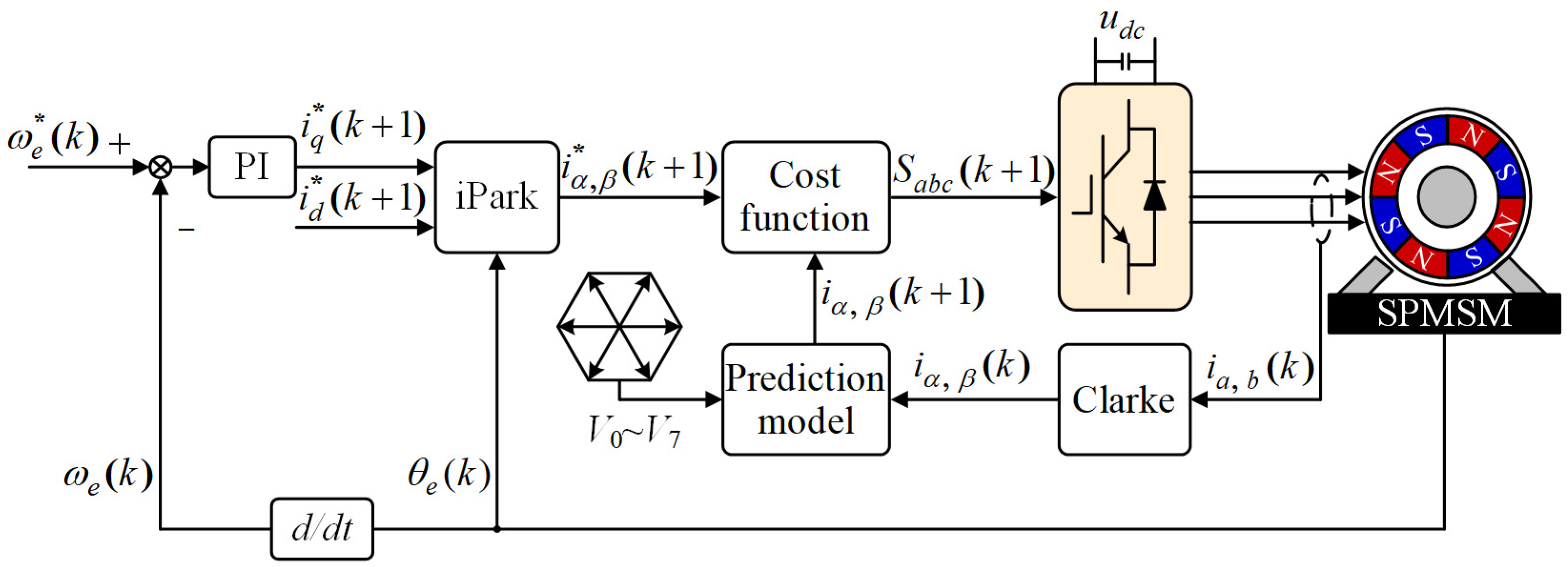
2. Basic Principle of FCS-MPCC

Within the stationary two-phase reference frame, the mathematical model of the surface-mounted permanent-magnet synchronous motor (SPMSM) is expressed as follows:
d i α d t = 1 L s ( u α R s i α e α ) d i β d t = 1 L s ( u β R s i β e β )
where Rs and Ls denote the stator resistance and inductance. uα and uβ signify the α- and β-stator voltage components; iα and iβ signify the α- and β-stator current components; eα and eβ signify the α- and β-back electromotive force (EMF) components, which can be formulated as
e α = ω e ψ f sin θ e e β = ω e ψ f cos θ e
where ωe signifies the rotor electrical angular velocity; θe signifies the rotor electrical position; ψf signifies the flux linkage. FCS-MPCC treats current as the primary control variable. Using the mathematical model of the SPMSM, the current responses under all switching states of the VSI are predicted. A cost function is then used to evaluate these predicted responses and determine the optimal switching state for the next control cycle. By applying the forward Euler method to discretize Equation (1), the current prediction model is formulated as
i α ( k + 1 ) = i α ( k ) + T s L s u α ( k ) R s i α ( k ) e α ( k ) i β ( k + 1 ) = i β ( k ) + T s L s u β ( k ) R s i β ( k ) e β ( k )
where k and k + 1 indicate the current and the succeeding sampling instances; Ts represents the control period; uα(k) and uβ(k) indicate the α- and β-axis stator voltage components within the kTs control period; iα(k) and iβ(k) indicate the α- and β-axis sampled current components at k instance; iα(k + 1) and iβ(k + 1) indicate the α- and β-axis predicted current components at k + 1 instance; eα(k) and eβ(k) indicate the α-and β-axis EMF components at k instance. When a three-phase two-level VSI is used, FCS-MPCC predicts the current response under eight basic voltage vectors using Equation (3). The candidate voltage vector set is then optimized through a cost function, as shown in (4):
g = [ i α * i α ( k + 1 ) ] 2 + [ i β * i β ( k + 1 ) ] 2
where i α * and i β * represent the reference current components in the α- and β-axes. The reference values are obtained using the rotor position and expressed as follows:
i α * = i d * cos θ e i q * sin θ e i β * = i d * sin θ e + i q * cos θ e
where id* denotes the d-axis reference current component and iq* denotes the q-axis reference current component. In the FCS-MPCC, the generation of the dq-axis reference currents idq*(k + 1) is a core aspect of the control strategy. This process must be designed considering the motor’s operational objectives (such as speed, torque, efficiency) and constraint conditions (such as voltage and current limits). The generation of the dq-axis reference currents is typically the output of the outer speed control loop. For the motor’s dual-loop control structure, the torque reference value of the motor was obtained through the speed loop proportional-integral (PI) controller based on the speed tracking error [9]. For the SPMSM, iq* = Te*/(1.5 npψf). Since 1.5 npψf can be included in the proportional gain, the q-axis current reference value iq* can be directly obtained from the speed loop PI controller. Moreover, in SPMSMs, the output torque is generated entirely by the q-axis current. To maximize torque production and prevent the formation of a reverse magnetic field, id* is typically set to zero, ensuring maximum motor efficiency [26]. Figure 1 presents the block diagram of FCS-MPCC.

3. An Improved MRAS-Based DV-MPCC

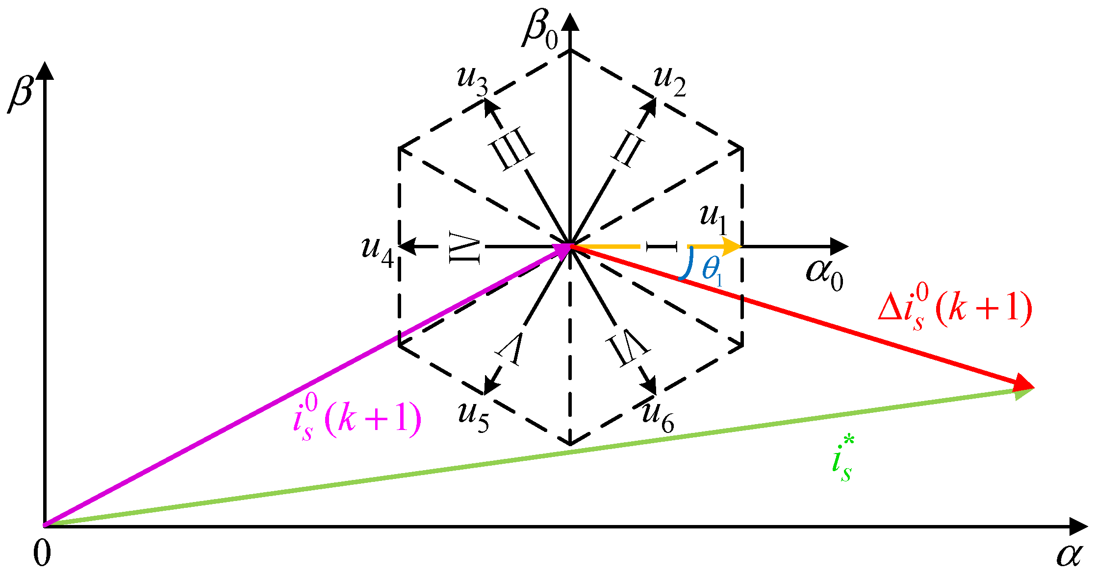
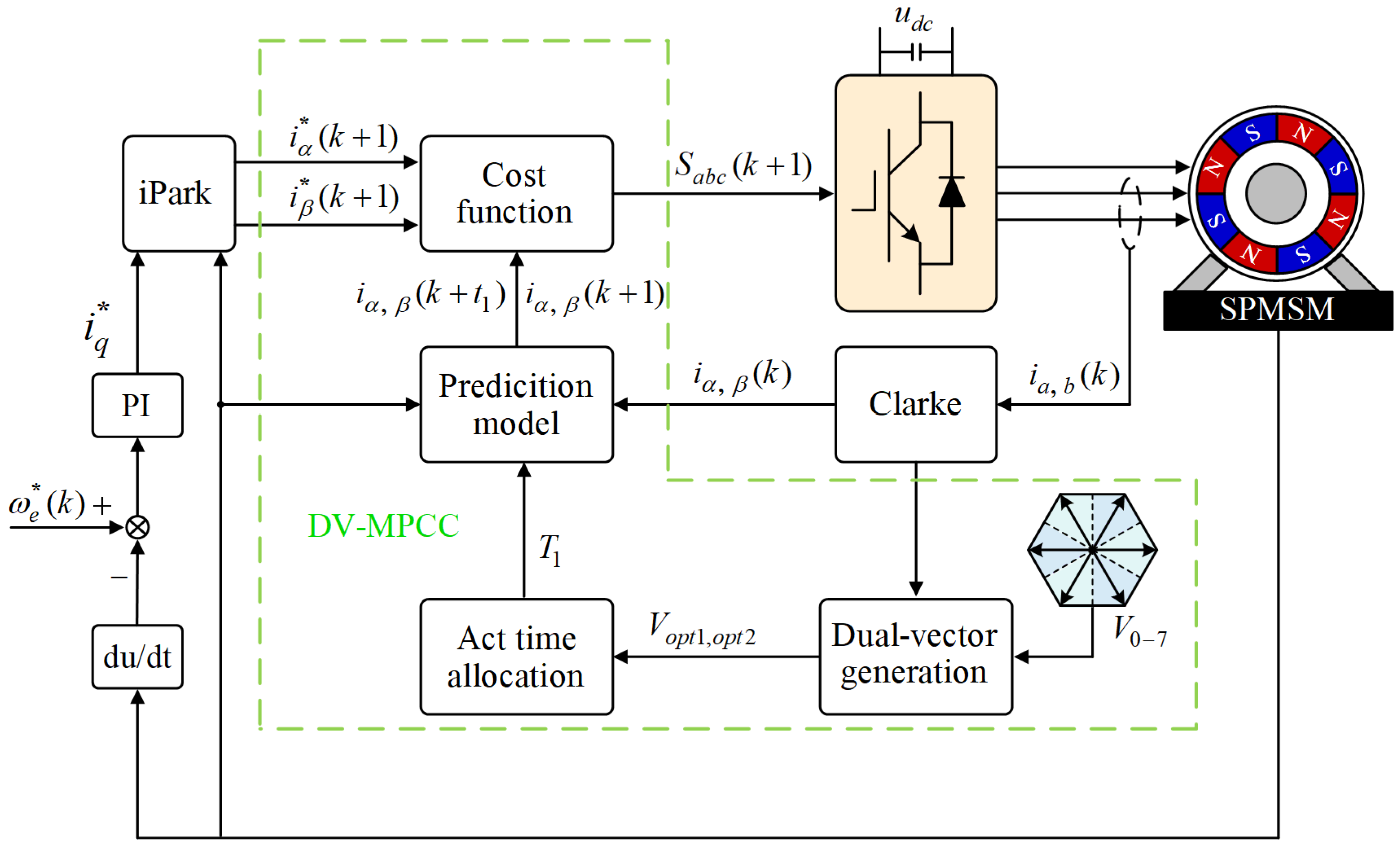
3.1. Error Current Vector-Based DV-MPCC

To achieve accurate reference current tracking and minimize overall current ripple, this section introduces a DV combination framework based on the error current vector. By analyzing the phase difference between the error current vector and the effective voltage vector, the proposed method directly selects the optimal effective voltage vector for precise current tracking. The selected voltage vector is the initial vector in the DV combination. It is then combined with the remaining six voltage vectors to generate a set of DV candidates. The detailed methodology is as follows. First, Equation (3) can be further reformulated as below:
i α ( k + 1 ) = T s L s u α ( k ) c o n t r o l l a b l e + ( 1 T s R s L s ) i α ( k ) T s L s e α ( k ) u n c o n t r o l l a b l e i β ( k + 1 ) = T s L s u β ( k ) c o n t r o l l a b l e + ( 1 T s R s L s ) i β ( k ) T s L s e β ( k ) u n c o n t r o l l a b l e
According to Equation (6), the predicted current consists of two components: a controllable term and an uncontrollable term. For the uncontrollable term, the current sampling value at the k instant is influenced by the voltage vector applied in the previous instant, while the EMF is determined by the rotor position and speed information at the k instant. Consequently, this term introduces an effect in the current control cycle that cannot be modified, resembling the application of a zero-voltage vector. In contrast, the controllable term accounts for the influence of the effective voltage vector applied in the present control cycle. The predicted current at the k + 1 instant, considering only the effect of the uncontrollable term, is given by the following:
i α 0 ( k + 1 ) = ( 1 T s R s L s ) i α ( k ) T s L s e α ( k ) i β 0 ( k + 1 ) = ( 1 T s R s L s ) i β ( k ) T s L s e β ( k )
The predicted current vector at the k + 1 instant under the effect of uncontrollable term can be noted as i s 0 ( k + 1 ) = [ i α 0 ( k + 1 ) i β 0 ( k + 1 ) ] T , and the given current vector can be described as i s * = [ i α * i β * ] T . The error current vector can be obtained by taking the difference between the predicted current vector and the reference current vector, which is noted as Δ i s 0 ( k + 1 ) = [ i α * i α 0 ( k + 1 ) i β * i β 0 ( k + 1 ) ] T . Under the effect of the controllable term, the error current vector Δ i s 0 ( k + 1 ) varies along with the direction of the applied effective voltage vector. Based on geometric and mathematical relationships, the distance between the predicted current vector—affected by different effective voltage vectors—and the reference current vector can be formulated as follows:
Δ i s j ( k + 1 ) = Δ i s 0 ( k + 1 ) 2 + ( T s L s u m ) 2 u n c o n t r o l l a b l e 2 T s L s u m Δ i s 0 ( k + 1 ) cos θ j c o n t r o l l a b l e
where um represents the magnitude of the effective voltage vector, and θj represents the phase difference between effective voltage vector and error current vector, j ∈ [1, 6]. By analyzing Equation (8), the magnitude of the error current vector Δ i s 0 ( k + 1 ) and um do not change with the application of different effective voltage vectors. Therefore, in Equation (8), this component can be considered an uncontrollable term, which remains positive. The separation between the predicted current vector and the reference current vector is always positive. To minimize this separation when applying an effective voltage vector, the controllable term in Equation (8) must be positive and maximized. This requirement can be equivalently expressed as −π/2 < θj < π/2, with θj being as close to 0 as possible. Based on the above analysis, a new α0-β0 coordinate system is constructed, where the endpoint of the predicted current vector under the influence of the zero-voltage vector is chosen as the coordinate system’s origin. As depicted in Figure 2, by following the principle of dividing the space into ±30° regions around the effective voltage vectors, the spatial plane is segmented into six regions.
When the error current vector falls within Sector I, the effective voltage vector u1 in this sector has the smallest angle θ1 relative to the error current vector. In this scenario, the controllable term in Equation (8) is positive and reaches its maximum. As a result, the predicted current vector, affected by u1, has the shortest distance to the reference current vector, ensuring optimal reference current tracking performance. Therefore, the first voltage vector in the DV combination is selected based on the sector in which the error current vector resides. Subsequently, this voltage vector is paired with the remaining six voltage vectors to form a candidate set for the DV combination.
Once all possible DV combinations are generated, it is necessary to allocate action times for each voltage vector. To address this, a vector action time allocation method is developed based on minimizing the RMSE of current tracking. The first and second voltage vectors in the DV combination are defined as Vopt1 and Vopt2, respectively. According to Equation (4), the current change rates at the k instant, under the influence of these voltage vectors, are determined as follows:
S α o p t 1 = u α o p t 1 ( k ) R s i α ( k ) e α ( k ) L s | V s = V o p t 1 S β o p t 1 = u β o p t 1 ( k ) R s i β ( k ) e β ( k ) L s | V s = V o p t 1
S α o p t 2 = u α o p t 2 ( k ) R s i α ( k ) e α ( k ) L s | V s = V o p t 2 S β o p t 2 = u β o p t 2 ( k ) R s i β ( k ) e β ( k ) L s | V s = V o p t 2
Define T1 as the first voltage vector action time. The RMSE of current tracking is deduced as
E = 1 T s 0 T 1 i α ( k ) i α * + S α o p t 1 t 2 d t   + 1 T s 0 T 1 i β ( k ) i β * + S β o p t 1 t 2 d t + 1 T s T 1 T s i α ( k ) i α * + S α o p t 1 T 1 + S α o p t 2 ( t T 1 ) 2 d t + 1 T s T 1 T s i β ( k ) i β * + S β o p t 1 T 1 + S β o p t 2 ( t T 1 ) 2 d t
To achieve the minimum RMSE of the current during motor operation, the condition dE/dt = 0 must be satisfied. Consequently, the duration of the first voltage vector can be calculated as
T 1 = B 1 + B 1 2 4 A 1 C 1 2 A 1
where A1, B1, and C1 are given in Equation (13). If T1 < 0, set T1 = 0; if T1 > Ts, set T1 = Ts. The vector action time allocation, determined using the aforementioned method, ensures that the motor exhibits reduced current ripple during operation. After generating the candidate DV set and allocating the durations of the voltage vectors, all DV combinations should be evaluated using a cost function. Define T1/Ts = t1, and k + t1 as the time instant of the DV switching point. To minimize current fluctuations, the cost function is formulated as shown in Equation (14):
A 1 = ( S α o p t 1 S α o p t 2 ) ( 2 S α o p t 1 S α o p t 2 ) ( S β o p t 1 S β o p t 2 ) ( 2 S β o p t 1 S β o p t 2 ) B 1 = 2 ( S α o p t 1 S α o p t 2 ) T s ( S α o p t 1 S α o p t 2 ) i α ( k ) + i α * + 2 ( S β o p t 1 S β o p t 2 ) T s ( S β o p t 1 S β o p t 2 ) i β ( k ) + i β * C 1 = T s ( S α o p t 1 S α o p t 2 ) T s S α o p t 2 + 2 i α ( k ) 2 i α * + T s ( S β o p t 1 S β o p t 2 ) T s S β o p t 2 + 2 i β ( k ) 2 i β *
g = g 1 + g 2 g 1 = [ i α * i α ( k + t 1 ) ] 2 + [ i α * i α ( k + 1 ) ] 2 g 2 = [ i β * i β ( k + t 1 ) ] 2 + [ i β * i β ( k + 1 ) ] 2
where iα(k + t1) and iβ(k + t1) represent the α- and β-axes’ predicted current components at the switching point, respectively. These components are calculated using the sampled currents iα(k) and iβ(k) at the k instant, combined with the effect of the voltage vector, as described by Equation (15). iα(k + 1) and iβ(k + 1) represent the α- and β-axes’ predicted components of the stator current at the k + 1 instant, which are determined according to Equation (16). Where uαopt1 (k) and uβopt1 (k) indicate the α- and β-axes’ components of the first voltage vector, while uαopt2 (k) and uβopt2 (k) indicate the α- and β-axes’ components of the second voltage vector. The block diagram of the proposed DV-MPCC is depicted in Figure 3.
i α ( k + t 1 ) = i α ( k ) + T 1 L s u α o p t 1 ( k ) R s i α ( k ) e α ( k ) i β ( k + t 1 ) = i β ( k ) + T 1 L s u β o p t 1 ( k ) R s i β ( k ) e β ( k )
i α ( k + 1 ) = i α ( k ) + T 1 L s u α o p t 1 ( k ) + T s T 1 L s u α o p t 2 ( k ) T s L s R s i α ( k ) + e α ( k ) i β ( k + 1 ) = i β ( k ) + T 1 L s u β o p t 1 ( k ) + T s T 1 L s u β o p t 2 ( k ) T s L s R s i β ( k ) + e β ( k )
DV-MPCC is a control strategy that depends on motor parameters, and its stability is influenced by these parameters. This section analyzed the impact of parameter mismatches on system stability by constructing a small-signal model of DV-MPCC. Since DV-MPCC used a cost function to select the optimal voltage vector combination, it was difficult to establish an accurate mathematical relationship between the optimal voltage vector and the stator current. This posed a significant challenge in constructing the small-signal model of DV-MPCC. To address this issue, the reference voltage vector was first calculated based on the current tracking principle, and the error between the reference voltage vector and the optimal voltage vector selected using the cost function was treated as an external disturbance, which does not affect the system’s stability. Based on this approach, the small-signal model of the DV-MPCC was constructed using the reference voltage vector. In the predictive model, when actual motor parameters were used, the reference voltage vector obtained from the current tracking principle could be expressed as follows:
u d * = R s i d ( k ) + L s i d * i d ( k ) T s ω e L s i q ( k ) u q * = R s i q ( k ) + L s i q * i q ( k ) T s + ω e L s i d ( k ) + ω e ψ f
When a motor parameter mismatch occurs, the reference voltage vector obtained based on the current tracking principle becomes the following:
u d m * = R s m i d ( k ) + L s m i d * i d ( k ) T s ω e L s m i q ( k ) u q m * = R s m i q ( k ) + L s m i q * i q ( k ) T s + ω e L s m i d ( k ) + ω e ψ f m
In the equation, R sm = R s + Δ R s , L sm = L s + Δ L s , and ψ fm = ψ f + Δ ψ f , where Δ R s , Δ L s ,   and   Δ ψ f represent the errors between the stator resistance, inductance, and permanent-magnet flux linkage parameters used in the predictive model under parameter mismatch and the actual motor parameters. Based on Equation (18), the equivalent block diagram of the MPCC under parameter mismatch can be constructed, as shown in Figure 4.
DV-MPCC can be considered a proportional control system that incorporates both feedforward and feedback terms. Its small-signal model can be expressed as
i d = ( ω e L s i q + u d ) 1 L s s + R s i q = ( ω e L s i d + u q ) 1 L s s + R s u d = ( R s m i d L s m T s i d ω e L s m i q ) 1 T s s + 1 u q = ( R s m i q L s m T s i q + ω e L s m i d ) 1 T s s + 1
where i d   and   i q represent the small disturbances of the stator current components along the d- and q-axes, respectively; u d and u q represent the small disturbances of the stator voltage components along the d- and q-axes. By reconstructing Equation (19), the state-space representation of the system can be derived.
d d t i d i q u d u q = R s L s ω e 1 L s 0 ω e R s L s 0 1 L s R s m T s L s m T s 2 ω e L s m T s 1 T s 0 ω e L s m T s R s m T s L s m T s 2 0 1 T s i d i q u d u q
According to linear system theory, the stability of the system can be assessed by analyzing the eigenvalues of the system’s state matrix from Equation (20). By varying the resistance and inductance parameters within the matrix, the system’s eigenvalue trajectories could be plotted. The system was considered stable only when all eigenvalues lie in the left half-plane. Figure 5 shows the eigenvalues of the system under different parameter mismatches. The symbol ∗ and ∘ represents the calculation results under the condition of accurate parameters. From the figure, the system became unstable when the stator resistance parameter used in the predictive model exceeded its actual value by a factor of 8. In practical scenarios, the stator resistance is influenced by the temperature of the stator winding. When the stator winding temperature changes from 25 °C to 100 °C, the resistance value only increases by approximately 1.3 times. Therefore, under normal operating conditions, variations in the resistance parameter did not affect the system’s stability. Furthermore, within the range where the stator inductance parameter varied from 0.1 to 10 times its nominal value, all eigenvalues remained in the left half-plane, indicating that inductance parameter mismatch does not cause system instability. However, when there was a large error in the stator inductance parameter, the system became more sensitive, leading to an increase in current harmonic content. Additionally, the back EMF could be treated as an external disturbance, which does not affect the system’s stability.

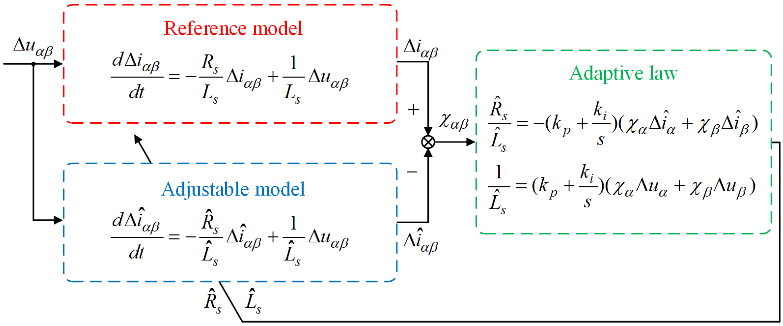
3.2. Incremental State Equation-Based MRAS Parameter Identification Method

DV-MPCC is a control strategy based on the motor model, which requires motor parameters for the current prediction process. When discrepancies exist between the parameters used in the current prediction model and the actual parameters, corresponding errors are introduced, leading to a degradation in control performance. To address this challenge, an enhanced parameter identification method based on the MRAS is introduced.
Traditional MRAS-based parameter identification methods construct an adjustable model based on Equation (1). However, when the parameter identification method relies on an underdetermined adjustable model, using only a single set of input and output variables is insufficient to ensure the accurate convergence of the identified values to the actual values. As a result, without injecting additional signals, Equation (1) can only be used to identify two parameters, leading to an underdetermined problem in parameter identification. The flux linkage parameter in the adjustable model should initially be set to its nominal value, allowing the stator resistance and inductance parameters to be estimated in parallel. Under these conditions, the state equation reduces to a second-order equation containing only two unknown machine parameters, thus avoiding the underdetermined problem. However, nominal values are typically obtained from the motor’s technical datasheet, and many motor manufacturers do not provide motor parameters. Furthermore, discrepancies between the nominal and actual parameter values can lead to inaccurate identification results.
To address these issues, this section proposed an MRAS-based multi-parameter estimation method utilizing the incremental current state equation. The core concept of this method was to construct an incremental current state equation that did not involve the flux linkage parameter. This incremental state equation was used as the adjustable model in the MRAS framework to estimate the stator resistance and inductance parameters, ensuring that the identification results were unaffected by the flux linkage parameter. The current differential equations at the current and previous instants are given by Equations (21) and (22), respectively.
Δ i α ( k ) T s = R s L s i α ( k 1 ) + 1 L s [ u α ( k 1 ) e α ( k 1 ) ] Δ i β ( k ) T s = R s L s i β ( k 1 ) + 1 L s [ u β ( k 1 ) e β ( k 1 ) ]
Δ i α ( k 1 ) T s = 1 L s [ u α ( k 2 ) e α ( k 2 ) ] R s L s i α ( k 2 ) Δ i β ( k 1 ) T s = 1 L s [ u β ( k 2 ) e β ( k 2 ) ] R s L s i β ( k 2 )
Since the motor’s mechanical time constant was significantly larger than the electrical time constant, the rotor speed was considered constant over successive control periods. As a result, the change in the electrical angle between two adjacent control periods was minimal, leading to negligible variations in the back EMF between adjacent control periods. Therefore, the variation in the back EMF term was insignificant compared to the variation in the voltage term. By subtracting Equation (22) from Equation (21), the incremental current state equation is derived as follows:
Δ i α ( k ) Δ i α ( k 1 ) T s = 1 L s Δ u α ( k 1 ) R s L s Δ i α ( k 1 ) Δ i β ( k ) Δ i β ( k 1 ) T s = 1 L s Δ u β ( k 1 ) R s L s Δ i β ( k 1 )
where Δuα(k − 1) = uα(k − 1) − uα(k − 2) indicates the α-axis incremental voltage at the k − 1 instant; Δuβ(k − 1) = uβ(k − 1) − uβ(k − 2) indicates the β-axis incremental voltage at the k − 1 instant; Δiα(k) = iα(k) − iα(k − 1) indicates the α-axis incremental current at the k instant; Δiβ(k) = iβ(k) − iβ(k − 1) indicates the β-axis incremental current at the k instant; Δiα(k − 1) = iα(k − 1) − iα(k − 2) represents the α-axis incremental current at the k − 1 instant; Δiβ(k − 1) = iβ(k − 1) − iβ(k − 2) represents the β-axis incremental current at the previous instant. The rank of the incremental current state equation is 2, and it does not involve the flux linkage parameter. This state equation can be used to construct an adjustable model for the identification of resistance and inductance parameters. According to MRAS theory and Equation (23), the reference and adjustable models for resistance and inductance parameter identification are given by Equations (24) and (25), respectively.
d d t Δ i α Δ i β = R s L s 0 0 R s L s Δ i α Δ i β + 1 L s 0 0 1 L s Δ u α Δ u β
d d t Δ i ^ α Δ i ^ β = R ^ s L ^ s 0 0 R ^ s L ^ s Δ i ^ α Δ i ^ β + 1 L ^ s 0 0 1 L ^ s Δ u α Δ u β
where R ^ s and L ^ s represent the identified values of the resistance and inductance parameters. Based on Equations (24) and (25), as well as the Popov hyperstability theory, the adaptive laws were formulated using a PI structure. Accordingly, the adaptive laws for identifying the R ^ s / L ^ s and 1 / L ^ s parameters are obtained as follows:
R ^ s L ^ s = k p ( χ α Δ i ^ α + χ β Δ i ^ β ) k i 0 t ( χ α Δ i ^ α + χ β Δ i ^ β ) d t
1 L ^ s = k p ( χ α Δ u α + χ β Δ u β ) + k i 0 t ( χ α Δ u α + χ β Δ u β ) d t
where χ α β = χ α χ β T = Δ i α Δ i ^ α Δ i β Δ i ^ β T . The proposed method enabled accurate identification of both resistance and inductance parameters. The block diagram of the incremental state equation-based MRAS parameter identification method is shown in Figure 6.
According to Equations (15) and (16), the flux linkage parameter is embedded within the back EMF. To prevent the degradation of DV-MPCC performance caused by mismatches in the permanent-magnet flux linkage parameter, this study adopts a back EMF calculation method that does not require the flux linkage parameter [26,27]. Utilizing the estimated resistance and inductance parameters and Equation (4), the EMF can be directly calculated using the reconstructed voltage and the sampled current.
e α ( k 1 ) = u α ( k 1 ) R ^ s i α ( k 1 ) L ^ s i α ( k ) i α ( k 1 ) T s e β ( k 1 ) = u β ( k 1 ) R ^ s i β ( k 1 ) L ^ s i β ( k ) i β ( k 1 ) T s
where uα(k − 1) and uβ(k − 1) represent the α- and β-axis stator voltage components applied during the (k − 1)Ts control period. iα(k − 1) and iβ(k − 1) denote the α- and β-axis components of the sampled stator current at the k − 1 instant. eα(k − 1) and eβ(k − 1) denote the α- and β-axis components of the EMF at the k − 1 instant. Since the motor’s mechanical time constant is significantly larger than the electrical time constant, and DV-MPCC is typically implemented at a high control frequency to ensure steady-state current tracking performance, the rotor speed can be considered as constant over successive control periods. Under this assumption, the back EMF at the previous instant can be approximated as equal to that at the current instant. Therefore, directly calculating the back EMF helps avoid current prediction errors caused by mismatches in the flux linkage parameter.

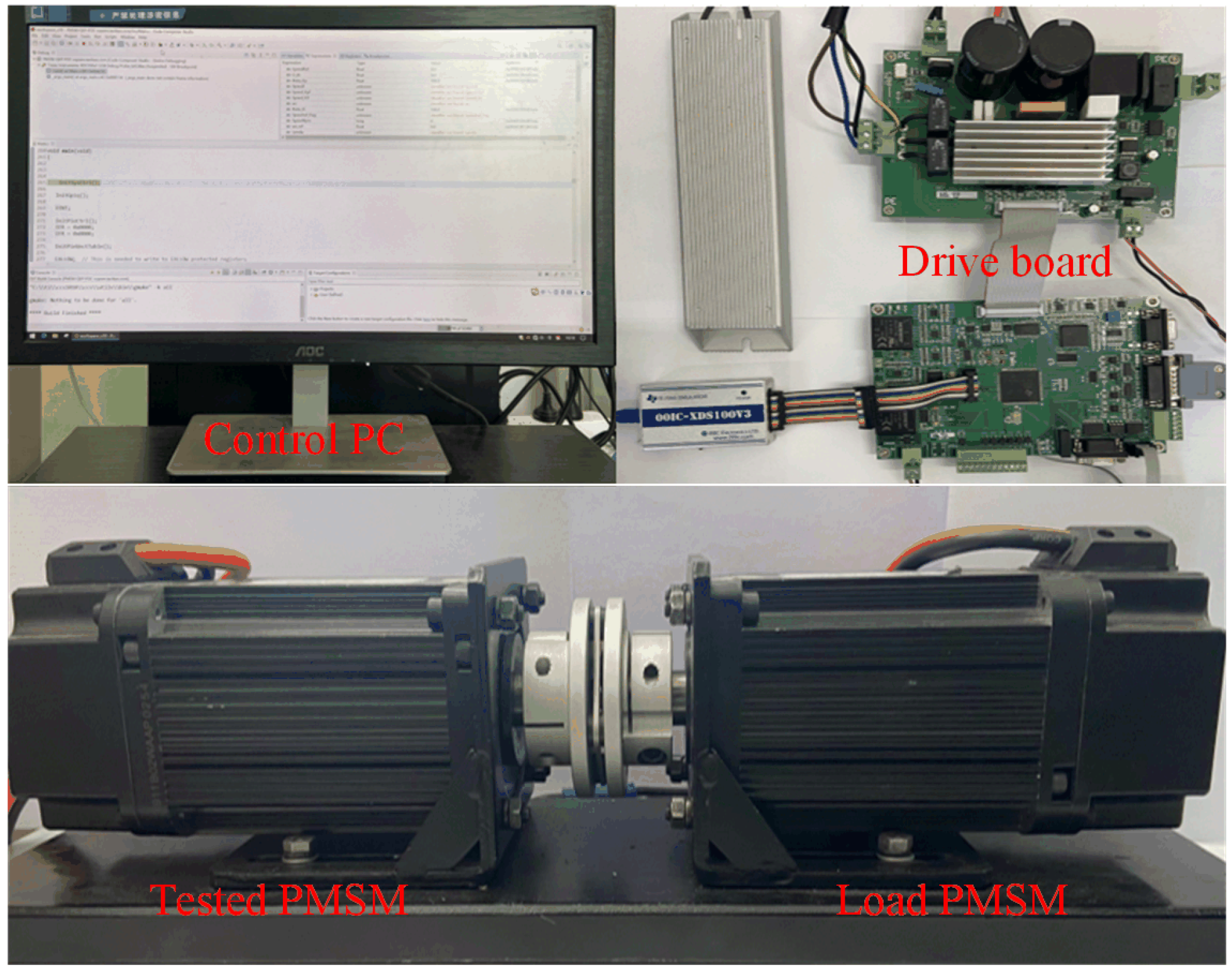
4. Experimental Validations

The effectiveness of the proposed strategy is demonstrated using the PMSM test platform shown in Figure 7. The motor parameters are listed in Table 1.

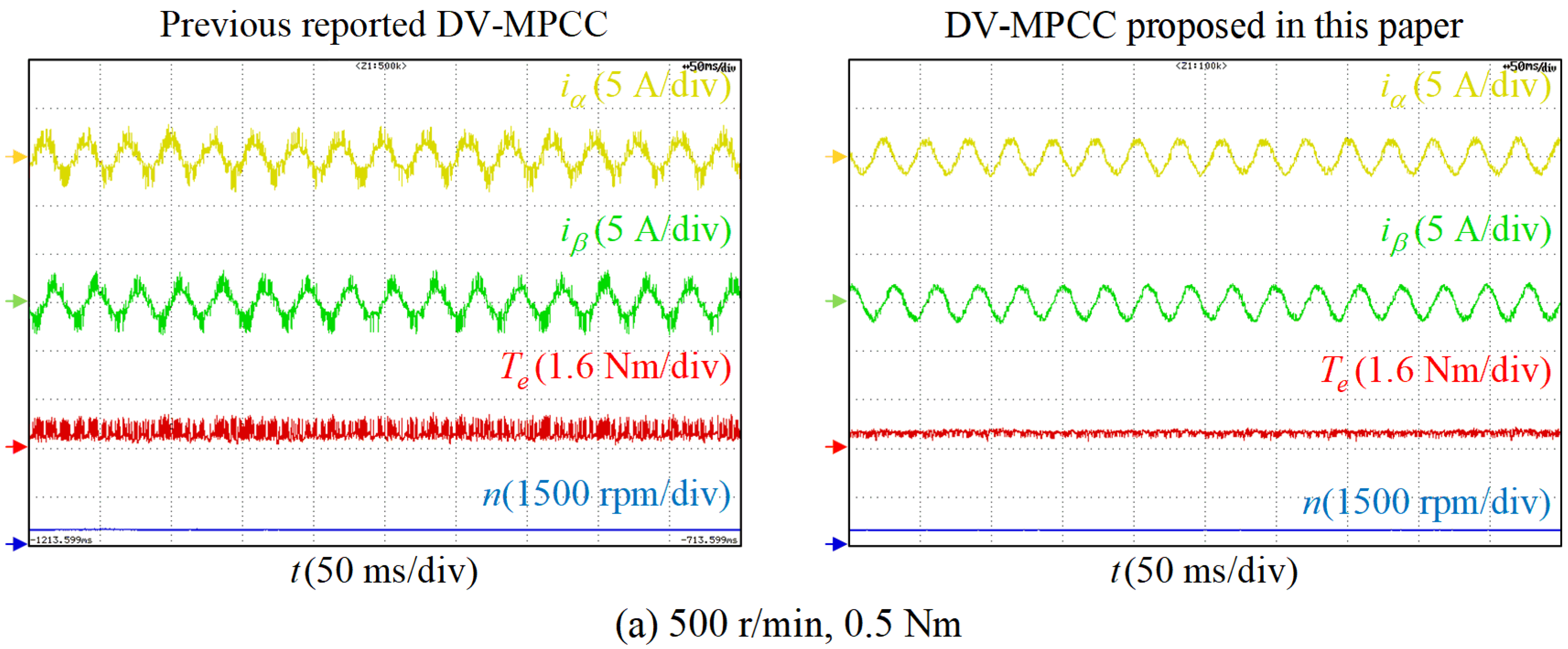
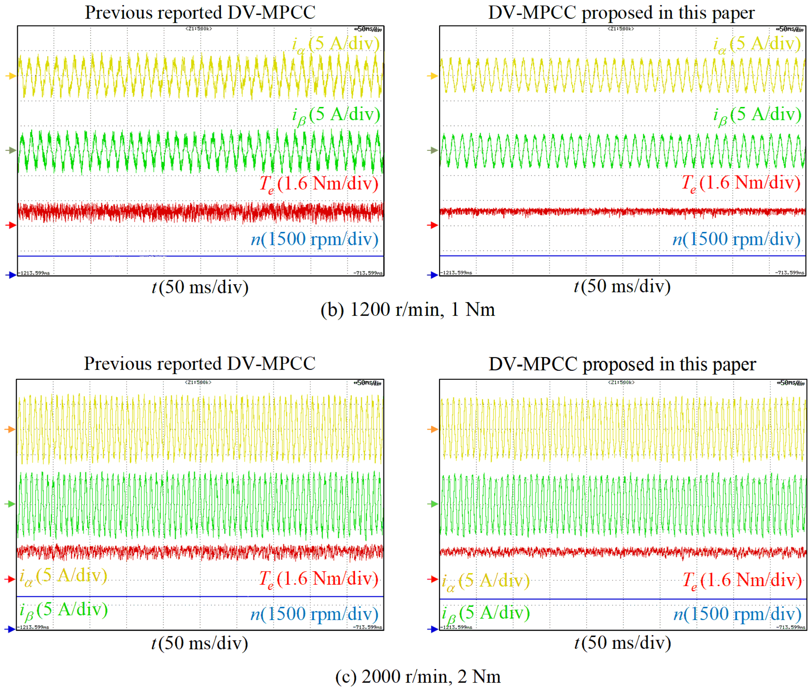
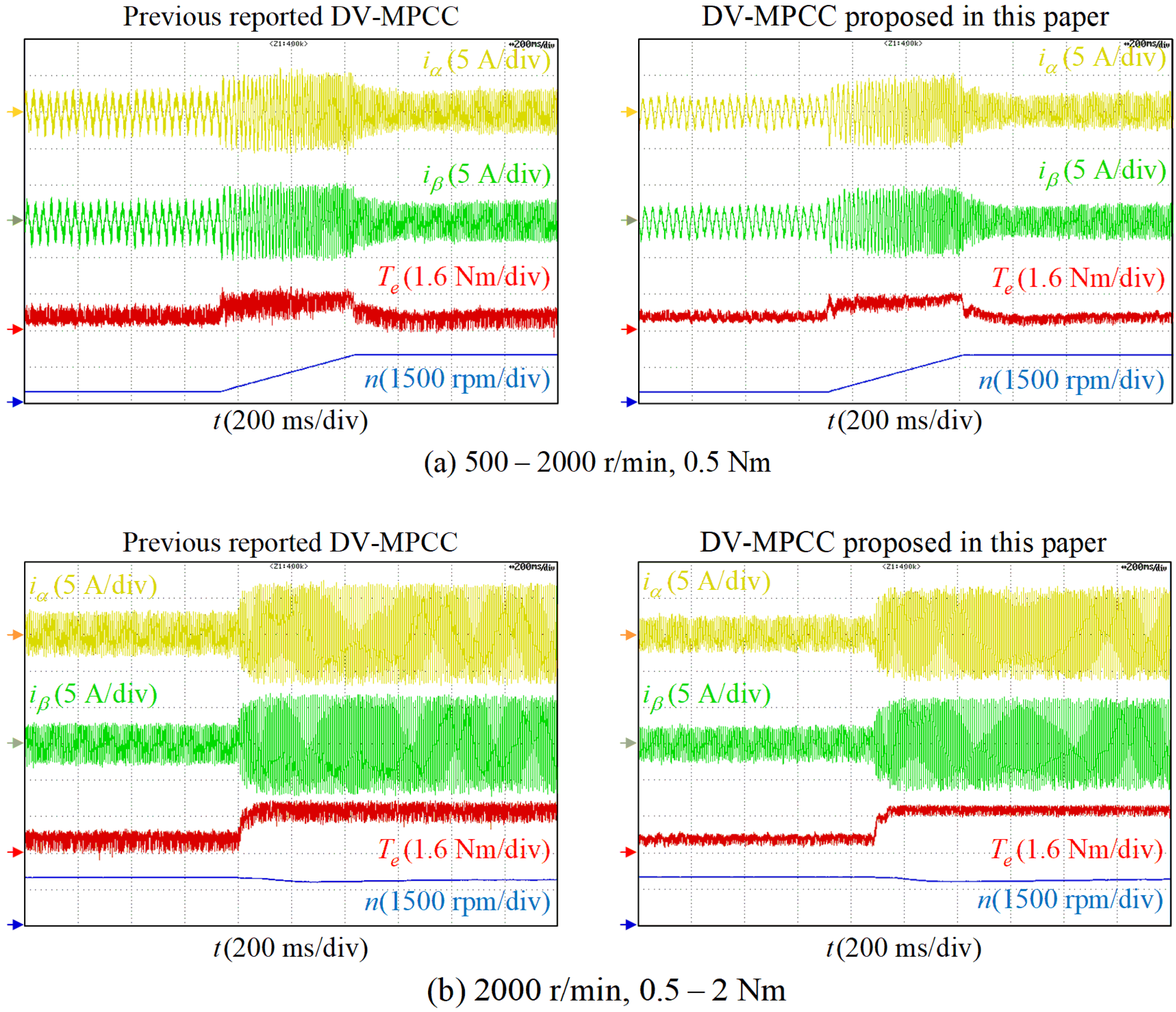
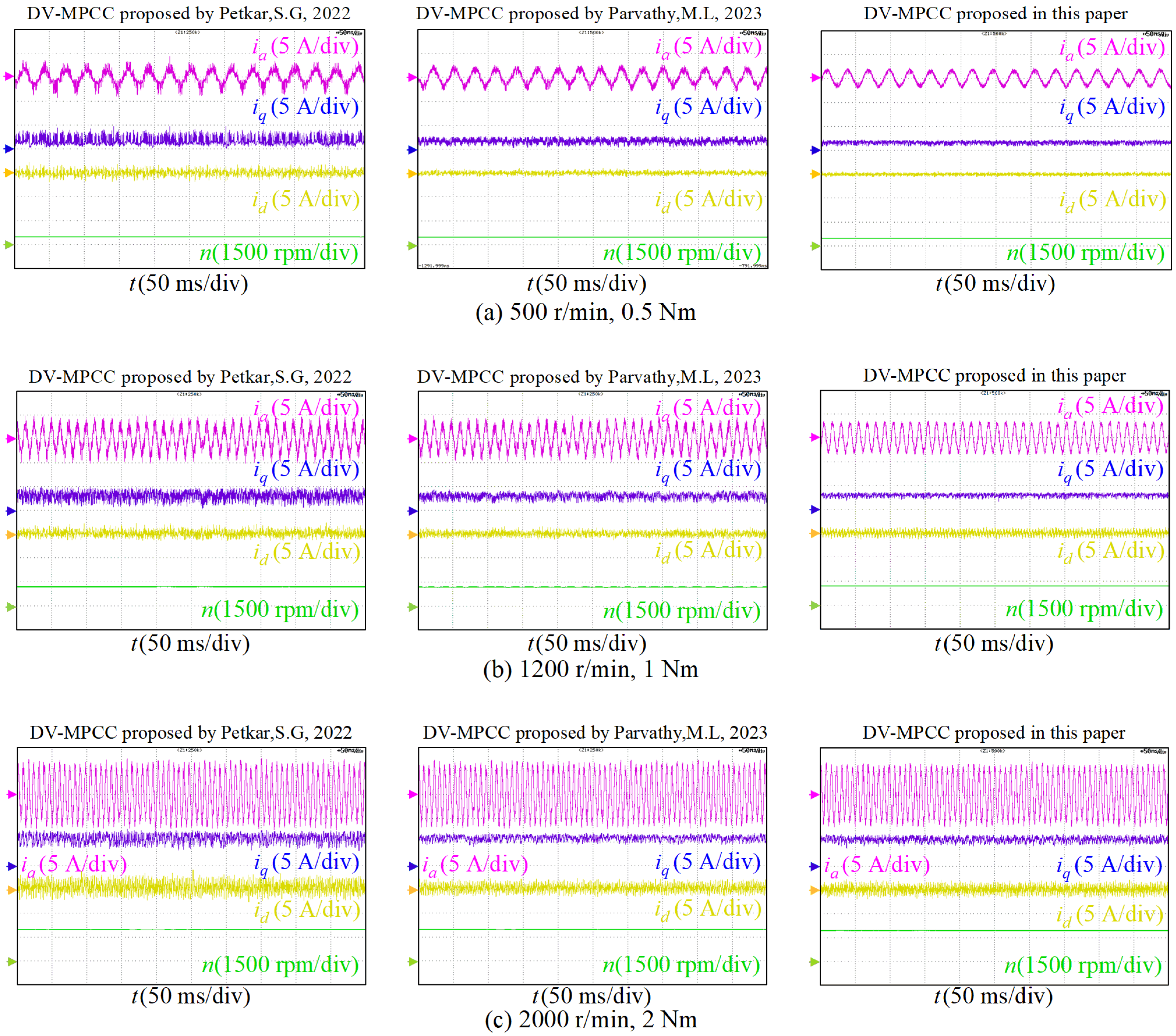
4.1. Improved DV-MPCC Control Performance Validation

To verify that the proposed DV-MPCC improves both control performance and computational efficiency during steady-state operation, a performance comparison was made between the previous reported DV-MPCC method [9] and the proposed DV-MPCC method. The tested SPMSM was operated under three steady-state conditions: 500 rpm with a light load, 1200 rpm with a medium load, and 2000 rpm with a high load. The experimental waveforms corresponding to these conditions are presented in Figure 8.
Since both control strategies are implemented in the two-phase stationary reference frame, the standard deviation of the d- and q-axis currents was not appropriate for evaluating steady-state control performance. Therefore, torque ripple and the total harmonic distortion (THD) of the phase current were used as efficiency metrics. Under the three operating conditions mentioned above, the torque ripple of the DV-MPCC method was 0.401 Nm, 0.567 Nm, and 0.443 Nm, respectively [9]. Using a power quality analyzer, the THD of the A-phase current was measured as 21.9%, 24.4%, and 20.7%, respectively. In contrast, the torque ripple of the proposed DV-MPCC was 0.238 Nm, 0.279 Nm, and 0.284 Nm, with corresponding THD values of 15.8%, 16.7%, and 18.4%. Compared to the DV-MPCC method [9], the proposed DV-MPCC reduced torque ripple by 40.6%, 50.8%, and 35.9%, and decreased current THD by 27%, 24%, and 19%, respectively. These results indicated that the proposed DV-MPCC significantly enhanced the motor’s steady-state operation performance.
In addition, a comparison of computational efficiency between the DV-MPCC method [9] and the proposed method in this paper was conducted. A flag was set to 1 before the DV-MPCC algorithm executed and reset to 0 after its completion. By observing the duty cycle of the flag signal, the execution times of the two algorithms were compared. The experimental results, presented in Figure 9, showed that the execution time of the DV-MPCC algorithm was approximately 26.5 µs, whereas the execution time of the proposed DV-MPCC algorithm was approximately 16.5 µs, representing a 37.7% reduction in execution time [9]. These results demonstrated that the proposed DV combination method significantly improved computational efficiency.
To demonstrate that the proposed DV-MPCC method preserves the dynamic response speed of the DV-MPCC [9], a comparison was conducted under conditions of acceleration and load variation. The experimental results are shown in Figure 10. Initially, with a load of 0.5 Nm, the speed was step-increased from 500 rpm to 2000 rpm. Once the motor reached steady-state operation at 2000 rpm, the load was step-increased from 0.5 Nm to 2 Nm. The results revealed that, following the sudden change in reference speed, the proposed DV-MPCC completed the acceleration process within 0.6 s, with minimal current fluctuation and virtually no overshoot. Similarly, after the reference torque changed, the proposed DV-MPCC handled the load increase in just 0.15 s. These findings suggest that the proposed DV-MPCC successfully maintains the dynamic control performance of the method [9]. A control performance comparison of the DV-MPCC proposed in [9] and that proposed in this paper is also shown in Table 2.
To further evaluate the proposed DV-MPCC method’s ability to enhance steady-state control performance, its performance was compared with the strategies under different steady-state operating conditions [10,11]. The experimental results are shown in Figure 11. Since the strategies were implemented in the d-q rotating reference frame [10,11], the controlled variables (α- and β-axis currents) in the proposed DV-MPCC method were transformed into d- and q-axis currents to ensure a fair comparison. This allowed for a direct and intuitive comparison of steady-state control performance across the different DV-MPCC methods. The tested SPMSM was operated under three steady-state conditions: 500 rpm with a light load, 1200 rpm with a medium load, and 2000 rpm with a high load. Under these conditions, the q-axis current ripple of the DV-MPCC method was 0.995 A, 0.778 A, and 0.704 A, respectively [10]. The THD of the A-phase current, measured using a power quality analyzer, was 20.7%, 22.3%, and 19.8%, respectively. For the DV-MPCC method, the q-axis current ripple was 0.597 A, 0.466 A, and 0.436 A, respectively, with corresponding THD values of 19.4%, 18.5%, and 18.1% [11]. For the proposed DV-MPCC in this paper, the q-axis current ripple was 0.352 A, 0.410 A, and 0.365 A, respectively, with THD values of 16.1%, 16.9%, and 17.9%. These results indicated that the proposed DV-MPCC significantly improved the motor’s steady-state control performance. A control performance comparison of DV-MPCC as in [10], DV-MPCC as in [11], and that proposed in this paper is also shown in Table 3.

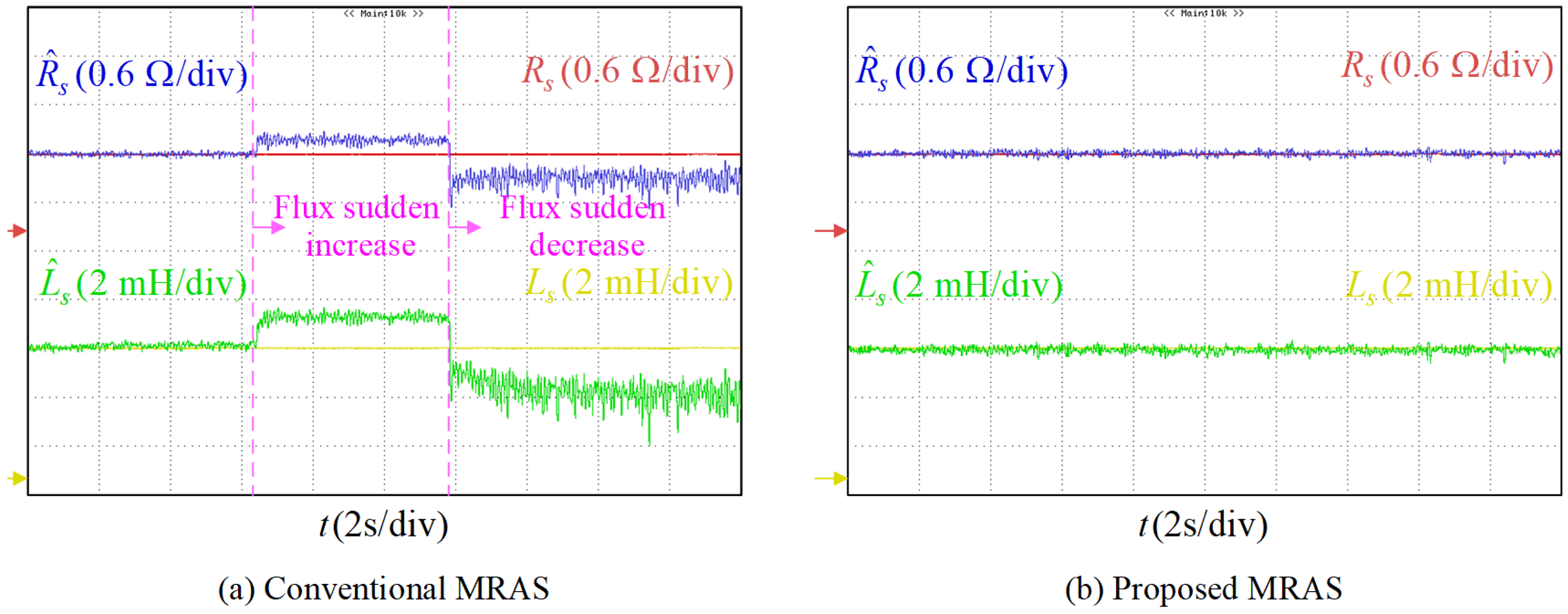
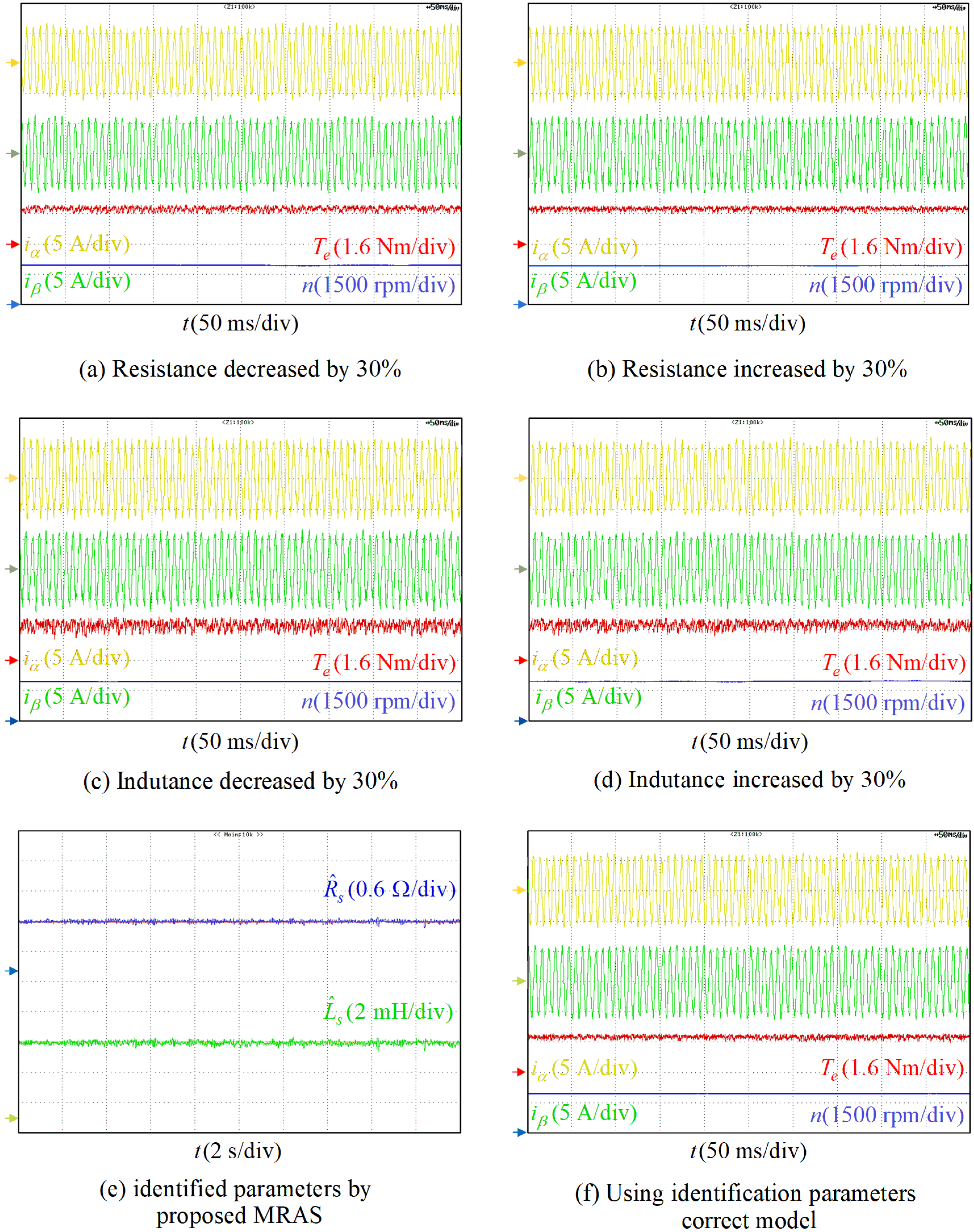
4.2. Improved MRAS Parameter Identification Performance Verification

Conventional MRAS methods cannot simultaneously identify all motor parameters due to the rank deficiency problem, which results in the flux linkage parameter of the adjustable model being fixed. To validate the impact of flux linkage parameter mismatch on the identification accuracy of other parameters, the motor was operated under no-load conditions at 500 rpm. In the reference model of the conventional MRAS method, the flux linkage parameter was set to 0.9 times and 1.1 times the actual value, respectively. The identification results for the stator resistance and inductance parameters are shown in Figure 12a. When the flux parameter was underestimated, the identified stator resistance and inductance values were significantly higher than their actual values. Specifically, the identified stator resistance exhibited an 8% error, while the stator inductance showed a 22% error. Conversely, when the flux parameter was overestimated, the identified stator resistance and inductance values were obviously lower than the actual values, with errors of 12% and 29%, respectively. This analysis showed that the error in the flux linkage parameter had a greater influence on the accuracy of inductance identification. However, the stator inductance plays a crucial role in DV-MPCC. Therefore, parameters identified using the conventional MRAS method with flux linkage parameter mismatch cannot meet the requirements for improving system parameter robustness. Figure 12b shows the identification results for stator resistance and inductance parameters when the motor operates at 500 rpm under no-load conditions using the improved MRAS method based on the motor’s incremental state equations. The identified average stator resistance is 0.905 Ω, with a 4.4% error, while the identified stator inductance is 5.483 mH, with a 5.1% error. These results demonstrated that the improved MRAS method could effectively estimate motor parameters. To further validate the disturbance rejection capability of the cascaded MRAS method, the motor was operated at 2000 rpm with a 2 Nm load. After the identified parameters stabilized, the estimated resistance and inductance values were suddenly altered, as shown in Figure 13. After the abrupt change, the values rapidly recovered within 80 ms, demonstrating the proposed method’s strong disturbance rejection capability and fast response time.
Figure 14a,b show the experimental results for the drive motor operating at 2000 rpm with a 2 Nm load, where the stator resistance parameter in the predictive model is set to 0.7 times and 1.3 times the actual value, respectively. Under these conditions, the torque ripple was 0.308 Nm and 0.291 Nm, showing no significant change compared to the case with accurate parameters. Figure 14c,d present the experimental results when the stator inductance parameter is set to 0.7 times and 1.3 times the actual value, respectively. In these cases, the torque ripple increased to 0.419 Nm and 0.366 Nm, representing an approximately 31.5% and 27.2% increase compared to the case with accurate parameters. Additionally, the current harmonic content increased under these conditions. However, when the motor parameters were identified and updated in the predictive model using the MRAS method based on the motor’s incremental state equations, the torque ripple was reduced to 0.287 Nm. Compared to the case with accurate parameters, there was no degradation in control performance, such as increased phase current harmonic content or heightened torque ripple.

5. Conclusions

This study investigated the DV-MPCC method with parameter identification. By analyzing the phase difference between the current tracking error and the effective voltage vector, it could be concluded that the best tracking performance was achieved when the phase difference between the effective voltage vector and the error current vector was less than 30°. Based on this finding, a DV combination method was designed using the error current vector, along with a time allocation strategy that minimizes the RMSE in current tracking. Compared to the DV-MPCC method with constrained switching states, the proposed DV-MPCC method based on the error current vector reduced torque ripple by 40%, thus enhancing steady-state control performance. Additionally, an MRAS parameter estimation method, derived from the incremental current state equations, was proposed. Using the identified parameters to update the model, the adverse effects of parameter mismatch were avoided. Unlike conventional MRAS parameter identification methods, the proposed method eliminated dependence on the nominal values of motor parameters and resolved the rank-deficiency problem without requiring the injection of additional excitation signals.
Furthermore, the tuning process for the parameters kp and ki in the adaptive law of MRAS lacks clear theoretical guidance, often necessitating empirical adjustments based on practical engineering to meet control performance requirements. The parameters kp and ki significantly influenced the identification process. As these parameters increased, the convergence speed of the identification algorithm accelerated. However, the noise within the parameters also increased, leading to reduced identification accuracy. In practical applications, selecting adaptive law parameters requires balancing convergence speed and accuracy, aiming for faster identification while maintaining acceptable precision. In future work, the author plans to employ fuzzy control for adjusting adaptive law parameters, eliminating the need for repetitive trial-and-error approaches based on engineering experience.

Author Contributions

Conceptualization, Y.Z. and S.H.; methodology, S.H.; software, L.S.; validation, S.H., Y.Z. and L.S.; formal analysis, B.C.; investigation, S.H.; resources, S.H.; data curation, S.H.; writing—original draft preparation, S.H.; writing—review and editing, S.H. and Y.H.; visualization, S.H.; supervision, Y.H.; project administration, S.H.; funding acquisition, S.H. All authors have read and agreed to the published version of the manuscript.

Funding

This research was funded by [Green Intelligent Ship Standardization Leading Project—2030 Green Intelligent Coastal and Inland River Demonstration Ship—2030 Fujian Green Intelligent Ship Key Technology and Demonstration Ship Development] grant number [Civilian Product Research—Ministry of Industry and Information Technology (Fujian Shipbuilding)—23K155-280] And The APC was funded by [Green Intelligent Ship Standardization Leading Project—2030 Green Intelligent Coastal and Inland River Demonstration Ship—2030 Fujian Green Intelligent Ship Key Technology and Demonstration Ship Development].

Data Availability Statement

Data are contained within the article.

Conflicts of Interest

The authors declare no conflict of interest.

References

  1. Han, X.; Yao, X.L.; Liao, Y.F. Full Operating Range Optimization Design Method of LLC Resonant Converter in Marine DC Power Supply System. J. Mar. Sci. Eng. 2023, 11, 2142. [Google Scholar] [CrossRef]
  2. Kim, S.; Jeon, H. Comparative Analysis on AC and DC Distribution Systems for Electric Propulsion Ship. J. Mar. Sci. Eng. 2022, 10, 559. [Google Scholar] [CrossRef]
  3. Zhou, Y.H.; Zhao, W.X.; Ji, J.H.; Zhu, S.D.; Hu, Q.Z. Zeroth-Order Vibration Analysis and Mitigation in Integral-Slot IPMSMs by Rotor Static Modulation Theory for Electrified Ship Propulsion. IEEE Trans. Transp. Electrif. 2024, 10, 7667–7678. [Google Scholar] [CrossRef]
  4. Mirzaeva, G.; Mo, Y.X. Model Predictive Control for Industrial Drive Applications. IEEE Trans. Ind. Appl. 2023, 59, 7897–7907. [Google Scholar] [CrossRef]
  5. Elmorshedy, M.F.; Xu, W.; El-Sousy, F.F.M.; Islam, M.R.; Ahmed, A.A. Recent Achievements in Model Predictive Control Techniques for Industrial Motor: A Comprehensive State-of-the-Art. IEEE Access. 2021, 9, 58170–58191. [Google Scholar] [CrossRef]
  6. Li, T.; Sun, X.D.; Lei, G.; Guo, Y.G.; Yang, Z.B.; Zhu, J.G. Finite-Control-Set Model Predictive Control of Permanent Magnet Synchronous Motor Drive Systems—An Overview. IEEE/CAA J. Autom. Sin. 2022, 9, 2087–2105. [Google Scholar] [CrossRef]
  7. Morel, F.; Lin-Shi, X.F.; Retif, J.-M.; Allard, B.; Buttay, C. A Comparative Study of Predictive Current Control Schemes for a Permanent-Magnet Synchronous Machine Drive. IEEE Trans. Ind. Electron. 2009, 56, 2715–2728. [Google Scholar] [CrossRef]
  8. Zhang, Y.C.; Yang, H.T. Generalized two-vector-based model-predictive torque control of induction motor drives. IEEE Trans. Power Electron. 2015, 30, 3818–3829. [Google Scholar] [CrossRef]
  9. Zhang, Y.C.; Yang, H.T. Two-vector-based model predictive torque control without weighting factors for induction motor drives. IEEE Trans. Power Electron. 2016, 31, 1381–1390. [Google Scholar] [CrossRef]
  10. Petkar, S.G.; Thippiripati, V.K. Enhanced Predictive Current Control of PMSM Drive with Virtual Voltage Space Vectors. IEEE J. Emerg. Sel. Top. Power Electron. 2022, 3, 834–844. [Google Scholar] [CrossRef]
  11. Parvathy, M.L. An Effective Modulated Predictive Current Control of PMSM Drive with Low Complexity. IEEE J. Emerg. Sel. Top. Power Electron. 2023, 10, 4565–4575. [Google Scholar] [CrossRef]
  12. Ma, C.W.; Rodríguez, J.; Garcia, C.; De Belie, F. Integration of Reference Current Slope Based Model-Free Predictive Control in Modulated PMSM Drives. IEEE J. Emerg. Sel. Top. Power Electron. 2023, 11, 1407–1421. [Google Scholar] [CrossRef]
  13. Zhang, X.G.; Zhang, L.; Zhang, Y.C. Model predictive current control for PMSM drives with parameter robustness improvement. IEEE Trans. Power Electron. 2019, 34, 1645–1657. [Google Scholar] [CrossRef]
  14. Rafaq, M.S.; Jung, J.W. A comprehensive review of state-of-the-art parameter estimation techniques for permanent magnet synchronous motors in wide speed Range. IEEE Trans. Ind. Informat. 2020, 16, 4747–4758. [Google Scholar] [CrossRef]
  15. Lian, C.Q.; Xiao, F.; Liu, J.L.; Gao, S. Parameter and VSI Nonlinearity Hybrid Estimation for PMSM Drives Based on Recursive Least Square. IEEE Trans. Transp. Electrific. 2023, 9, 2195–2206. [Google Scholar] [CrossRef]
  16. Li, X.Y.; Kennel, R. General formulation of kalman-filter-based online parameter identification methods for VSI-fed PMSM. IEEE Trans. Ind. Electron. 2021, 68, 2856–2864. [Google Scholar] [CrossRef]
  17. Odhano, S.A.; Pescetto, P.; Awan, H.A.A.; Hinkkanen, M.; Pellegrino, G.; Bojoi, R. Parameter Identification and Self-Commissioning in AC Motor Drives: A Technology Status Review. IEEE Trans. Power Electron. 2019, 34, 3603–3614. [Google Scholar] [CrossRef]
  18. Usama, M.; Kim, J. T Robust adaptive observer-based finite control set model predictive current control for sensorless speed control of surface permanent magnet synchronous motor. Trans. Inst. Meas. Control. 2021, 43, 1416–1429. [Google Scholar] [CrossRef]
  19. Usama, M.; Choi, Y.O.; Kim, J. Speed Sensorless Control based on Adaptive Luenberger Observer for IPMSM Drive. In Proceedings of the IEEE 19th International PEMC, Gliwice, Poland, 25–29 April 2021; pp. 602–607. [Google Scholar]
  20. Liu, Z.H.; Wei, H.L.; Li, X.H. Global identification of electrical and mechanical parameters in PMSM drive based on dynamic self-learning PSO. IEEE Trans. Power Electron. 2018, 33, 10858–10871. [Google Scholar] [CrossRef]
  21. Boileau, T.; Leboeuf, N.; Nahid-Mobarakeh, B.; Meibody-Tabar, F. Online Identification of PMSM Parameters: Parameter Identifiability and Estimator Comparative Study. IEEE Trans. Ind. Appl. 2011, 47, 1944–1957. [Google Scholar] [CrossRef]
  22. An, X.K.; Liu, G.H.; Chen, Q.; Zhao, W.X.; Song, X.J. Adjustable Model Predictive Control for IPMSM Drives Based on Online Stator Inductance Identification. IEEE Trans. Ind. Electron. 2022, 69, 3368–3381. [Google Scholar] [CrossRef]
  23. Nalakath, S.; Preindl, M.; Emadi, A. Online multi-parameter estimation of interior permanent magnet motor drives with finite control set model predictive control. IET Electri Power Appl. 2017, 11, 944–951. [Google Scholar] [CrossRef]
  24. Wang, L.; Zhang, S.; Zhang, C.; Zhou, Y. An Improved Deadbeat Predictive Current Control Based on Parameter Identification for PMSM. IEEE Trans. Transp. Electrific. 2024, 10, 2740–2753. [Google Scholar] [CrossRef]
  25. Liu, Y.; Ran, Q.; Zhao, S.P. Parameter Identification of Permanent Magnet Synchronous Motor Based on Improved MRAS Algorithm. J. Phys. Conf. Ser. 2023, 2456, 012050. [Google Scholar] [CrossRef]
  26. Zhang, Y.C.; Xu, D.L.; Liu, J.L. Performance improvement of model-predictive current control of permanent magnet synchronous motor drives. IEEE Trans. Ind. Appl. 2017, 53, 3683–3695. [Google Scholar] [CrossRef]
  27. Sun, X.D.; Hu, C.C.; Lei, G. Speed sensorless control of SPMSM drives for EVs with a binary search algorithm-based phase-locked loop. IEEE Trans. Veh. Technol. 2020, 69, 4968–4978. [Google Scholar] [CrossRef]
Figure 1. Block diagram of FCS–MPCC in two–phase stationary reference frame.
Jmse 13 00585 g001
Figure 2. Schematic diagram of selection method for effective voltage vectors.
Jmse 13 00585 g002
Figure 3. A block diagram of the proposed DV-MPCC in the stationary coordinate system.
Jmse 13 00585 g003
Figure 4. Equivalent block diagram of DV-MPCC.
Jmse 13 00585 g004
Figure 5. Small-signal eigenvalue loci with different mismatches of stator inductance and resistance.
Jmse 13 00585 g005
Figure 6. Block diagram of incremental state equation-based MRAS parameter identification.
Jmse 13 00585 g006
Figure 7. PMSM test platform.
Jmse 13 00585 g007
Figure 8. Steady-state control performance comparison of previous reported DV-MPCC method [9] and that proposed in this study.
Jmse 13 00585 g008aJmse 13 00585 g008b
Figure 9. Comparison of algorithm execution time.
Jmse 13 00585 g009
Figure 10. Dynamic-state control performance comparison of previous reported DV-MPCC method [9] and that proposed in this study.
Jmse 13 00585 g010
Figure 11. Steady-state control performance comparison between previous reported DV-MPCC methods [10,11] and that proposed in this paper.
Jmse 13 00585 g011
Figure 12. Identification performance comparison of conventional MRAS and proposed MRAS.
Jmse 13 00585 g012
Figure 13. Identification performance of proposed MRAS when identified parameters change.
Jmse 13 00585 g013
Figure 14. The impact of parameter mismatch and the control performance enhancement of the proposed DV-MPCC method with IMRAS.
Jmse 13 00585 g014
Table 1. Parameters of surface-mounted permanent-magnet synchronous motor.
ParameterVariableValue
PkW0.75
np/4
RsΩ0.901
LsmH5.445
ψfWb0.113
Tsμs100
UdcV311
TNNm2.4
Table 2. Control performance comparison of DV-MPCC proposed in [9] and this paper.
Performance
Metric
DV-MPCC Proposed in [9]DV-MPCC Proposed in This PaperPerformance
Improvement
Steady-state
performance
500 rpm,
light load
Te Ripple: 0.401 Nm
ia THD: 21.9%
Te Ripple: 0.238 Nm
ia THD: 15.8%
Ripple: 40.6% reduction; THD: 27% reduction
1200 rpm,
middle load
Te Ripple: 0.567 Nm
ia THD: 24.4%
Te Ripple: 0.279 Nm
ia THD: 16.7%
Ripple: 50.8% reduction; THD: 24% reduction
2000 rpm,
high load
Te Ripple: 0.443 Nm
ia THD: 20.7%
Te Ripple: 0.284 Nm
ia THD: 18.4%
Ripple: 35.9% reduction; THD: 19% reduction
Dynamic-state
performance
Acceleration response time0.6 s0.6 sRemains consistent
Load variation response time0.15 s0.15 sRemains consistent
Execution Time26.5 us16.5 us38% reduction
Table 3. Control performance comparison of DV-MPCC proposed in [10,11] and in this paper.
Steady-State
Performance
DV-MPCC Proposed in [10]DV-MPCC Proposed in [11]DV-MPCC Proposed in This Paper
500 rpm,
light load
iq Ripple: 0.995 A
ia THD: 20.7%
iq Ripple: 0.597 A
ia THD: 19.4%
iq Ripple: 0.352 A
ia THD: 16.1%
1200 rpm,
middle load
iq Ripple: 0.778 A
ia THD: 22.3%
iq Ripple: 0.466 A
ia THD: 18.5%
iq Ripple: 0.410 A
ia THD: 16.9%
2000 rpm,
high load
iq Ripple: 0.704 A
ia THD: 19.8%
iq Ripple: 0.436 A
ia THD: 18.1%
iq Ripple: 0.365 A
ia THD: 17.9%
Disclaimer/Publisher’s Note: The statements, opinions and data contained in all publications are solely those of the individual author(s) and contributor(s) and not of MDPI and/or the editor(s). MDPI and/or the editor(s) disclaim responsibility for any injury to people or property resulting from any ideas, methods, instructions or products referred to in the content.

