Nonlinear Sliding-Mode Super-Twisting Reaching Law for Unmanned Surface Vessel Formation Control Under Coupling Deception Attacks

Abstract

In this paper, a nonlinear sliding-mode super-twisting reaching law algorithm is designed to address the problem of coupling interference under deception attacks and actuator physical faults in USV formations during cooperative mining operations of a USVs-ROVs system. First, a USV model with attacks and disturbances is established, and a leader–follower formation system is designed. Then, based on the reaching law, the state error dynamic chatter can be effectively solved when it is far away from and reaches the sliding surface; a nonlinear sliding super-twisting reaching law is designed to improve the chatter characteristics of the sliding surface. Furthermore, to solve the problems of low fitting accuracy regarding control anomaly information and the difficulty of fending off signal-data interference attacks, a nonlinear saturation fault-tolerant filtering mechanism and a nonlinear fitting factor are designed. Finally, the stability of the algorithm is verified through Lyapunov theory. Under the same coupling deception probability, the nonlinear sliding-mode super-twisting reaching law algorithm designed in this paper enables the leader ship and each follower ship to reach stability within about 12s, and the formation system maintains its formation while also improving the control accuracy of each individual ship.

1. Introduction

In recent years, with the booming development of commercial, scientific, and military marine activities, intelligent devices such as Unmanned Surface Vessels (USVs) and Remote Operated Vehicle (ROVs) have played a crucial role in related engineering projects [1,2]. At present, they are a key tool for maritime transportation, playing an irreplaceable role in core tasks such as rescue missions, natural resource exploration, environmental monitoring, and maritime ship replenishment [3]. As terrestrial mineral resources are gradually depleted, the abundant mineral resources in the ocean, such as polymetallic nodules, cobaltrich crusts, and polymetallic sulfides, have become important potential sources to meet the continuous development needs of industry. Compared with operations using only USVs, the USVs-ROVs cooperative formation has better fault tolerance and adaptability [4], and its effectiveness in underwater missions largely depends on precise and reliable positioning and efficient control strategies [5]. Therefore, the control of USV formations is very important to ensure the safe navigation and efficient execution of the preset tasks of USVs-ROVs systems for collaborative mining operations.

Cooperative formation control of unmanned surface vehicles (USVs) differs from single-ship trajectory tracking due to the need to maintain a predetermined formation. Various methodologies exist, with the leader–follower approach standing out due to its simplicity and practicality. Ding et al. [6] conducted an in-depth study of surface vessel formation using this method, where one ship leads while others follow, turning the challenge into a coordination issue among followers relative to the leader. Lu et al. [7] explored leader–follower coordination under uncertain dynamics and external disturbances. Lin et al. [8] utilized observers to mitigate unknown disturbances, dividing ships into virtual leaders and followers, and simplified the controller design by transforming it into three subsystems. In USV-ROV cooperation, multiple uncertain factors affect stability and operational effectiveness, including natural phenomena like wind, waves, and currents. Van [9] enhanced tracking performance by combining adaptive integral sliding control with a disturbance observer. Martin et al. [10] designed model-based controllers for ROV tracking tasks. Ma et al. [11] proposed an adaptive integral sliding-mode control method based on an extended observer to address false data injection attacks. Li et al. [12] improved trajectory tracking in work-class ROVs using a fuzzy adaptive controller considering thruster dynamics. Tieshan Li et al. [13] introduced a nonlinear sliding-mode control method for underdriven ship formations, achieving the desired pattern within a limited time using finite-time stability theory. Chen et al. [14] established a nonlinear dynamic model, proposed a disturbance observer for uncertainty and external interference estimation and compensation, and designed a sliding-mode controller for good tracking performance. Yang et al. [15] used a fuzzy sliding-mode control method with a recurrent neural network (RNN) to stabilize ROV motion under uncertainties and disturbances. The RNN estimated ROV uncertainties, while the fuzzy logic system reduced chattering in sliding-mode control. Actuator faults can also affect controller performance. Schauer et al. [16] proposed a Hybrid Situation Awareness (HSA) model integrating physical and network situational awareness to detect and respond to composite attacks in maritime critical infrastructure. Li et al. [17] introduced SecureSSE, enhancing the robustness of autonomous ship sea state estimation models against adversarial attacks by integrating multi-scale feature extraction, feature convolution aggregation, and perturbation sample training modules. Zhang et al. [18] proposed an event-triggered algorithm based on robust neural damping and dynamic surface control to address actuator failure and model uncertainty in dynamically positioned ships, verified by experiments under complex sea conditions.

As collaborative mining operations of USV and ROV systems expand, they face not only natural disturbances but also heightened cyber vulnerabilities due to reliance on network communication technology [19]. Recent maritime incidents worldwide caused by cyber attacks highlight severe security concerns [20]. Various network attacks, including denial of service, deception, and replay attacks, pose significant threats. Muhammed Erbas et al. [21] reviewed ship network security, emphasizing the need for standardization, tool support, and expert verification to bolster cyber resilience. Kimberly Tam et al. [22] simulated cyber-physical attacks on container ship rudders, revealing risks to port operations and throughput, and proposed mitigation strategies. J Bhatti et al. [23] analyzed GPS spoofing risks and developed a detection framework to mitigate hostile ship control, validated through sea trials. Gao et al. [24] addressed USV collaboration in target tracking under event-triggered communication and DoS attacks. MS Mahmoud et al. [25] noted that deception attacks replace genuine data packets, misleading control centers. Moreover, physical actuator failures and deep-sea emergencies further complicate USV-ROV operations. Actuator saturation or malfunction in USVs disrupts fleet efficiency, while ROVs in extreme conditions face communication failures, sensor malfunctions, and mechanical damage. Juha Ubaleht [26] proposed enhancing GNSS anti-interference for autonomous ships using multi-source positioning and redundancy. Mahmoud Elsisi et al. [27] introduced an IoT system integrating drones and deep learning for emission monitoring, effectively detecting adversarial attacks with high accuracy. Although significant progress has been made in the control of USVs under normal operating conditions, the integration of path planning for trajectory tracking remains a key challenge. Previous research has focused on path planning algorithms in dynamic environments. Anete Vagale et al. [28] reviewed the path planning and collision avoidance technologies of autonomous surface vehicles, focusing on the related algorithms, challenges, and improvements in safety and operational efficiency. They also proposed a classification of path planning algorithms to provide a direction for future research. To combat coupling deception attacks, various methods have been proposed. Sung-Wook Ohn et al. [29] discussed the requirements of optimal path planning for autonomous ships, combining navigation practices with international collision avoidance rules (COLREGs), in order to improve the effectiveness of collision avoidance algorithms. Ho Namgung et al. [30] proposed a collision risk reasoning system based on ANFIS to help autonomous surface ships (MASS) optimize the timing and position of collision avoidance according to COLREG rules. But this ignores the coupling with guidance and control systems. Xiangyong Chen et al. [31] studied fixed-time synchronization for coupled neural networks using double-channel event-triggered control. Wenlong Yang et al. [32] addressed robust formation control in multi-agent systems with communication delays and uncertainties. Zhang C et al. [33] developed a preset performance super-sliding control for autonomous surface vehicles under external disturbances and modeling errors. Chengtao Feng et al. [34] proposed an adaptive super-twisting sliding control to improve trajectory tracking in unmanned vessels. Wenji Liu et al. [35] achieved stabilization control using a super-twisting expansion state observer, though not for trajectory tracking. Yancheng Liu et al. [36] designed a virtual control law and controllers using super-twisting sliding control to address overshoot in under-driven ship trajectory tracking, but did not consider complex uncertainties. Inspired by the above literature, the importance of USVs in marine transportation and environmental monitoring, as well as the threats of deceptive attacks and actuator failures, is clear; despite significant progress, challenges remain. The focus of this paper is to improve USV-ROV cooperative systems by designing a nonlinear sliding-mode super-twisting reaching law, enhancing fault tolerance and stability to ensure more reliable operation in critical maritime tasks. Therefore, this paper mainly contributes to the formation of USVs in the following ways:

(1)

A new nonlinear sliding-mode surface is designed for nonlinear fitting modeling of attacks coupled with actuator failures. Due to the physical limitation of system control ability, the redundancy information is saturated to improve the robustness of the system.

(2)

Based on the traditional approach law, a nonlinear super-twisting reaching law is designed. The nonlinear time-varying gain can be adjusted according to the system state, which effectively solves the dynamic change of error when it approaches and reaches the sliding surface, and can better control the sliding surface and reduce jitter.

(3)

In order to solve the saturation filtering problem, a dynamic error of the saturation filter is designed, and an adaptive nonlinear fault-tolerant filtering control mechanism is introduced to effectively deal with coupling attacks and actuator failures, to improve system stability and control accuracy.

2. Formation Model and Related Theory

2.1. USV Model

This paper studies the problem of USV formation control. It assumes that the USV model is clear and the parameters of the USV system are known. The global model for USV kinematics and dynamics is presented below [37]:

$$\dot{q}=J\left(\theta \right)v$$

(1)

$$M\dot{v}+C\left(v\right)v+Dv=\tau +{\overline{\tau }}_{df}$$

(2)

where $J\left(\theta \right)=[cos(\theta ),-sin(\theta ),0;sin(\theta ),cos(\theta ),0;0,0,1]$ is a transformation matrix for dynamics and kinematics in a coordinate system, where $J^{-1}\left(\theta \right)=J^{\mathrm{T}}\left(\theta \right)$ and $\parallel J_a\left({\theta }_a\right)\parallel =1$; $v={[u,v,r]}^{\mathrm{T}}$ is the velocity vector; and $\dot{q}={[\dot{x},\dot{y},\dot{\theta }]}^{\mathrm{T}}\in {\mathbb{R}}^{3\times 1}$ is the first-derivative vector of the position coordinate vector q. ${\tau }_u$ is the forward thrust of the ship, ${\tau }_v$ is the transverse lateral thrust, and ${\tau }_r$ is the bow rocking moment. They constitute the ship’s system inputs of $\tau ={[{\tau }_u,{\tau }_v,{\tau }_r]}^{\mathrm{T}}$. ${\overline{\tau }}_{df}={[{\overline{\tau }}_{df1},{\overline{\tau }}_{df2},{\overline{\tau }}_{df3}]}^{\mathrm{T}}$ is an external random disturbance of a USV, which has the characteristics of low frequency integrability. $M_a$ is a quality-related hydrodynamic additional relationship matrix, and $C\left(v\right)$ is Coriolis centripetal matrix; D is a hydrodynamic damping coefficient array. The matrix expressions are shown in Equations (3)–(5), respectively.

$$M_a=\left[\begin{array}{ccc}{m}_{11}& 0& 0\\ 0& m_{22}& m_{23}\\ 0& m_{32}& m_{33}\end{array}\right]$$

(3)

$$C\left(v\right)=\left[\begin{array}{ccc}0& 0& -m_{22}r-m_{23}w\\ 0& 0& m_{11}v\\ m_{22}r+m_{23}w& -m_{11}v& 0\end{array}\right]$$

(4)

$$D=\left[\begin{array}{ccc}{d}_{11}& 0& 0\\ 0& d_{22}& d_{23}\\ 0& d_{32}& d_{33}\end{array}\right]$$

(5)

where m is the quality of the USV; this USV is a symmetrical ship type with a left and right hull, which has the characteristic of the center of gravity and the origin of the appendage coordinate system being coincident.

2.2. Attack Model

In actual engineering tasks, the data transmission network from controllers to actuators is prone to random spoofing attacks and system uncertainty interference. Moreover, the actuators of USVs have physical saturation limitations, which can lead to physical failures. Therefore, an input nonlinear fitting model is introduced in advance for saturation fitting, and the hyperbolic tangent function is used to fit the saturation characteristics of shipboard actuators, with the actual input as follows:

$${\tau }_{\iota }\left(k\right)=A_{\tau }{\tau }_{max}tanh(\tau \left(k\right)+A_D)$$

(6)

where $\tau \left(k\right)$ is the online signal calculated by the controller, $A_{\tau }$ is an input local fault with coupling characteristics, and $A_D$ is a kind of covert data interference cyber attack. $A_D=\Im A_{\Im }$, where ℑ has the characteristics of independently distributed Bernoulli sequences of 0 or 1. $A_{\Im }$ is a virtual interference signal caused by an attack on the control signal.

The USV model is modeled with interference and attack items:

$$\left\{\begin{array}{c}\dot{q}=S\left(q\right)v\hfill \\ \dot{v}=\tilde{B}{\tau }_{\iota }\left(k\right)-\widehat{F}\left(\dot{q}\right)-\overline{\tau }\hfill \end{array}\right.$$

(7)

where $S\left(q\right)=[cos(\theta ),-sin(\theta ),0;sin(\theta ),cos(\theta ),0;0,0,1]$ is a transformation matrix for dynamics and kinematics in a coordinate system, with the characteristics of $S^{-1}\left(q\right)=S^{\mathrm{T}}\left(q\right)$; $\widehat{F}\left(\dot{q}\right)=M^{-1}C\left(v\right)v+M^{-1}Dv$ is a system uncertainty, $\overline{\tau }=M^{-1}{\overline{\tau }}_{df}$ is an external disturbance to the system, and $\tilde{B}=M^{-1}$ is the system control input conversion coefficient matrix.

In the actual operation process, USVs will face a series of physical constraints, such as the rated power of the actuators and the ship’s propeller. The actuators of each device also have physical saturation characteristics, so the saturation function is introduced to characterize and reconstruct the control input as follows:

$${\tau }_{si}=sat\left(\overline{{\tau }_i^a}\right)=\left\{\begin{array}{cc}\overline{{\tau }_i^a}\hfill & \parallel \overline{{\tau }_i^a}\parallel \le M_{\tau }\hfill \\ M_{\tau }\hfill & \overline{{\tau }_i^a}>M_{\tau }\hfill \end{array}\right.$$

(8)

where $M_{\tau }$ = ${\tau }_M$ = ${\tau }_{max}$ represents the constant absolute value of the physical saturation of the actuator, $M_{\tau }$ is the maximum allowable output of the actuator, and $sat(·)$ represents a saturation function. Combined with (6), the USV model with disturbance and attack terms morphs into

$$\left\{\begin{array}{c}\dot{q}=S\left(q\right)v\hfill \\ v=\tilde{B}sat\left(A_{\tau }{\tau }_{max}tanh(\tau \left(k\right)+A_D)\right)-\widehat{F}\left(\dot{q}\right)-\overline{\tau }\hfill \end{array}\right.$$

(9)

The control process of the formation system will be interfered with by factors such as physical faults of the actuator and deception attacks, which will produce unknown inputs and cause the control task to lose control. The nonlinear factor ${\eta }_{\tau }={\displaystyle \frac{A_{\tau }}{1+tanh\left(\tau \right)tanh\left(A_d\right)}}$ is designed to participate in the construction of the saturation mechanism. ${\eta }_f=1-{\eta }_{\tau }+{\eta }_{\tau }tanh\left(A_d\right)$ is introduced for decoupled linear processing of unknown inputs.

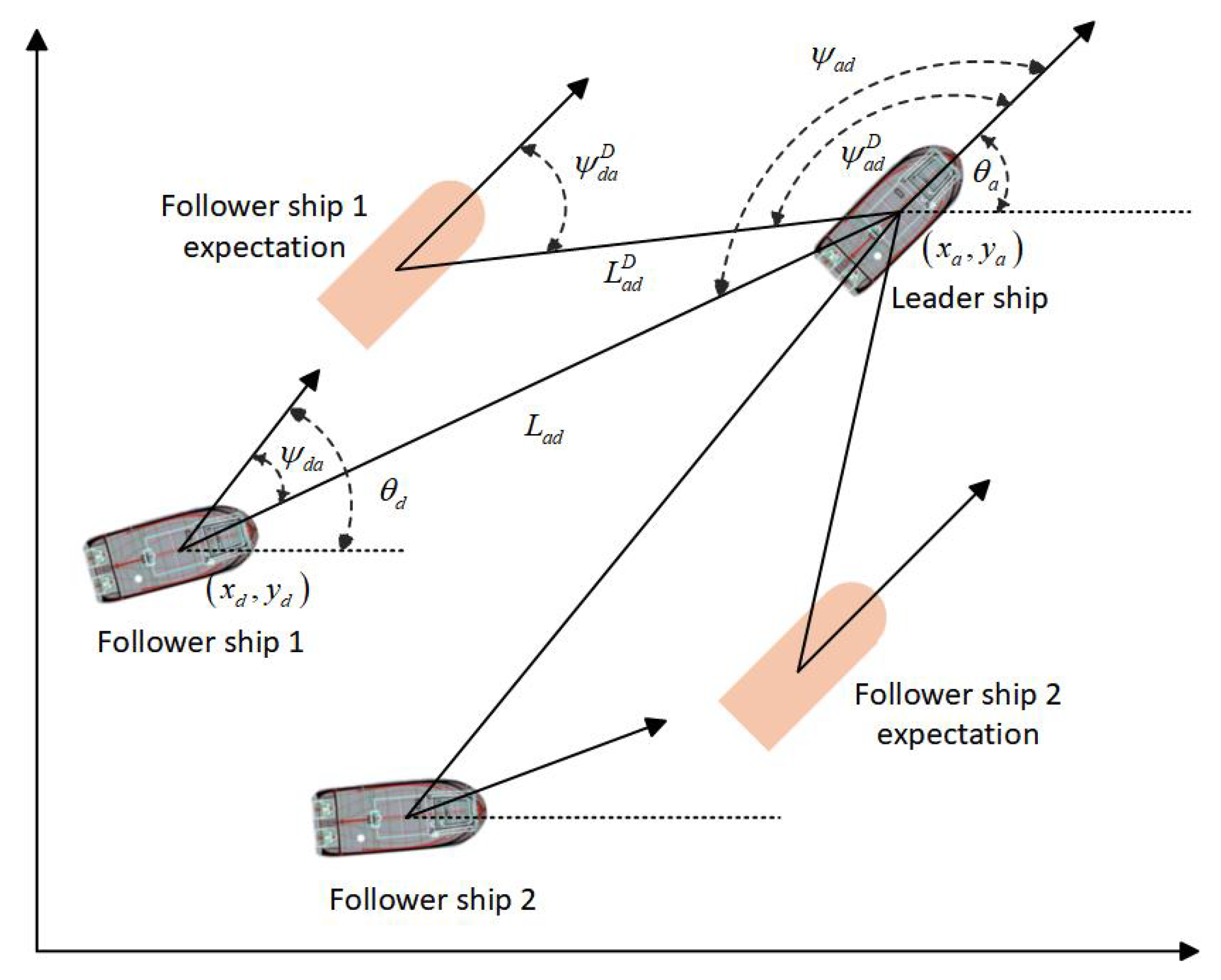
2.3. Formation Design

Inspired by other multi-agent formation research [38], this paper adopts the leader-following formation system. The following is a detailed description of the formation design for the leader ship and follower ship 1.

As shown in Figure 1, the expected formation geometric feature matrix of the leader and the follower is ${\Phi }_{ad}^D=[L_{ad}^D;{\psi }_{ad}^D;{\psi }_{da}^D]$. ${\psi }_{ad}^D$ and ${\psi }_{da}^D$ are the angles between the direction of the leader’s advance and the direction of the expected follower and the expected distance of $L_{ad}^D$, respectively. $L_{ad}^D$ is the desired geometric distance between the follower and the leader’s formation, $L_{ad}$ is the distance between the lead boat and the actual follower boat, ${\psi }_{ad}$ is the angle between the linear speed direction of the leader ship and the actual following distance, ${\psi }_{da}$ is the angle between the direction of the follower’s linear speed and the actual following distance, and the characteristic matrix of the true formation of the follower device and the leader device is ${\Phi }_{ad}=[L_{ad};{\psi }_{ad};{\psi }_{da}]$.

${\Phi }_{ad}$ is the formation geometry of the control system; when Formula (10) is satisfied, the cooperative control of formation geometry can be realized:

$$\underset{t\to \infty }{lim}({\Phi }_{ad}^D-{\Phi }_{ad})=0$$

(10)

From the Pythagorean theorem, we can see that there is $L_{ad}=\sqrt{L_{adx}^2+L_{ady}^2}$ between the generalized distance of the formation. We can decompose the formation distance into $L_{adx}$ and $L_{ady}$, as shown in Equation (11):

$$\left\{\begin{array}{c}{L}_{adx}=L_{ad}cos({\theta }_d-{\psi }_{da})=-L_{ad}cos({\theta }_a+{\psi }_{ad})\hfill \\ L_{ady}=L_{ad}sin({\theta }_d-{\psi }_{da})=-L_{ad}sin({\theta }_a+{\psi }_{ad})\hfill \end{array}\right.$$

(11)

The position relationship between followers and leaders is shown in Equation (12):

$$\left\{\begin{array}{c}{L}_{adx}=x_a-x_d\hfill \\ L_{ady}=y_a-y_d\hfill \\ {\psi }_{da}=\pi -{\theta }_a+{\theta }_d-{\psi }_{ad}\hfill \end{array}\right.$$

(12)

From Equation (11), we can obtain $arctan\left({\Delta }_d\right)=arctan\left({\Delta }_a\right)={\theta }_a-\pi +{\psi }_{ad}={\theta }_d-{\psi }_{da}$. Therefore, the relationship between the position of the equipment and the geometrical distance angle of the formation is

$$\left\{\begin{array}{c}{\psi }_{ad}=arctan\left({\Delta }_a\right)+\pi -{\theta }_a\hfill \\ {\psi }_{da}={\theta }_d-arctan\left({\Delta }_d\right)\hfill \end{array}\right.$$

(13)

The relationship between ${\Delta }_a$, ${\Delta }_d$, and the position of formation is the following:

$${\Delta }_a={\Delta }_d={\displaystyle \frac{L_{ady}}{L_{adx}}}={\displaystyle \frac{y_a-y_d}{x_a-x_d}}$$

(14)

From Equations (11)–(13), if the position of each single ship in the formation system is known, the formation geometry can be determined. It can be seen that the formation recovery movement in the formation scheme can be regarded as the coordinated tracking movement of the relative positions of multiple devices, and the relationship can be obtained as follows:

$$q_a=q_d+G_d$$

(15)

where, $q_d={[x_d,y_d,{\theta }_d]}^{\mathrm{T}}$ is the coordinate matrix of the follower, $q_a={[x_a,y_a,{\theta }_a]}^{\mathrm{T}}$ is the leader’s position coordinate matrix, and $G_d={[G_{dx},G_{dy},G_{d\theta }]}^{\mathrm{T}}$ is the formation coordinate transformation matrix. The transformation function matrix of coordinate x is $G_{dx}=L_{ad}cos({\theta }_d-{\psi }_{da})$, the transformation function matrix of coordinate y is $G_{dy}=L_{ad}sin({\theta }_d-{\psi }_{da}$, and the transformation function matrix of coordinate $\omega$ is $G_{d\theta }=\pi -{\psi }_{ad}-{\psi }_{da}$.

When $\underset{t\to \infty }{lim}(q_d+G_d-q_a)=0$, the formation restoration of the formation scheme is realized, and the definition of relative consistency of the geometric state is completed [39].

Formation movement coordination uses the geometric features of formation ${\Phi }_{ad}$ in the equipment movement process of the dynamic characteristics ${\dot{\Phi }}_{ad}$ to coordinate control, so as to achieve $\underset{t\to \infty }{lim}({\dot{\Phi }}_{ad}^D-{\dot{\Phi }}_{ad})=0$. Therefore, it is necessary to establish the dynamic relationship of formation geometry characteristics to describe the cooperative state of motion, and then coordinate control based on this relationship.

Taking the derivative of Equations (12) and (13) with respect to t, one can obtain the following:

$$\left\{\begin{array}{c}\begin{array}{c}{\dot{L}}_{adx}={\dot{x}}_a-{\dot{x}}_d=-{\dot{L}}_{ad}cos({\theta }_a+{\psi }_{ad})+L_{ad}({\omega }_a+{\dot{\psi }}_{ad})sin({\theta }_a+{\psi }_{ad})\hfill \\ {\dot{L}}_{ady}={\dot{y}}_a-{\dot{y}}_d=-{\dot{L}}_{ad}sin({\theta }_a+{\psi }_{ad})-L_{ad}({\omega }_a+{\dot{\psi }}_{ad})cos({\theta }_a+{\psi }_{ad})\hfill \\ {\dot{\psi }}_{ad}=L_{ad}^{-1}[({\dot{y}}_a-{\dot{y}}_d)cos({\theta }_a+{\psi }_{ad})+({\dot{x}}_a-{\dot{x}}_d)sin({\theta }_a+{\psi }_{ad})-{\omega }_a\hfill \\ {\dot{\psi }}_{da}={\omega }_d-L_{ad}^{-1}[({\dot{y}}_a-{\dot{y}}_d)cos({\theta }_d-{\psi }_{da})-({\dot{x}}_a-{\dot{x}}_d)sin({\theta }_d-{\psi }_{da})\hfill \end{array}\hfill \end{array}\right.$$

(16)

We take the derivative of the formation geometry relation $L_{ad}=\sqrt{L_{adx}^2+L_{ady}^2}$ with respect to t. Combined with (16), the geometric dynamic characteristics of the formation ${\dot{\Phi }}_{ad}=[{\dot{L}}_{ad};{\dot{\psi }}_{ad};{\dot{\psi }}_{da}]$ and the relationship between the position and dynamic characteristics of the leading ship and the following ship can be obtained.

In the above formula, the dynamic features of the formation include the dynamic features of each equipment position and the geometric features of the formation, so it can be seen that the coordination of formation movement is carried out synchronously with the coordination of formation geometry. And the final goal of motion coordination expressed by geometric dynamic features is the following:

$$\underset{t\to \infty }{lim}({\dot{\Phi }}_{ad}^D-{\dot{\Phi }}_{ad})=0$$

(17)

The relationship between the dynamic position and dynamic change characteristics of each ship is established, as shown in Equation (18):

$${\dot{q}}_a={\dot{q}}_d+G_{\dot{q}ad}=\left[\begin{array}{c}{\dot{x}}_a\\ {\dot{y}}_a\\ {\omega }_a\end{array}\right]=\left[\begin{array}{c}{\dot{x}}_d\\ {\dot{y}}_d\\ {\omega }_d\end{array}\right]+\left[\begin{array}{c}{G}_{\dot{x}ad}\\ G_{\dot{y}ad}\\ G_{\dot{\theta }ad}\end{array}\right]$$

(18)

where the motion transition term of x is $G_{\dot{x}ad}=-{\dot{L}}_{ad}cos({\theta }_a+{\psi }_{ad})+L_{ad}({\omega }_a+{\dot{\psi }}_{ad})sin({\theta }_a+{\psi }_{ad})$ and the motion transition term of y is $G_{\dot{y}ad}=-{\dot{L}}_{ad}sin({\theta }_a+{\psi }_{ad})-L_{ad}({\omega }_a+{\dot{\psi }}_{ad})cos({\theta }_a+{\psi }_{ad})$. The motion transition term of $\omega$ is $G_{\dot{\theta }ad}={\dot{\psi }}_{ad}+{\dot{\psi }}_{da}$.

To transform the formation cooperative control of the formation system into the motion cooperative control among all devices, the dynamic characteristics of the equipment can be transformed into the motion state of the equipment combined with the kinematic model, and the motion state is the motion coordination state, so the formation motion coordination can be realized. Then, the dynamic difference between the leader and the follower is

$$u_a=S_a^T\left(q_a\right)S_d\left(q_d\right)v_d+S_a^T\left(q_a\right)G_{\dot{q}ad}$$

(19)

According to the kinematic model, by sorting out Equation (19), the kinematic model of the formation movement coordination between the leader and the follower can be obtained as follows:

$$u_a=S_a^T\left(q_a\right)S_d\left(q_d\right)v_d+{\overline{G}}_{\dot{q}ad}$$

(20)

where ${\overline{G}}_{\dot{q}ad}=S_a^T\left(q_a\right)G_{\dot{q}ad}={[cos\left({\theta }_a\right)G_{\dot{x}ad}+sin\left({\theta }_a\right)G_{\dot{y}ad},-sin\left({\theta }_a\right)G_{\dot{x}ad}+cos\left({\theta }_a\right)G_{\dot{y}ad},G_{\dot{\theta }ad}]}^{\mathrm{T}}$ is the velocity state formation transition term.

By synthesizing the formation geometry coordination and formation motion coordination, the formation motion error model given in (20) is obtained, and the formation task is completed when the expected error is $\underset{t\to \infty }{lim}{\chi }_i^E=0$.

$${\chi }_i^E={\chi }_i^D-{\chi }_i^s=\left[\begin{array}{c}{\chi }_{\iota }^d\\ {\chi }_g^d\end{array}\right]-\left[\begin{array}{c}{\chi }_{\iota }\\ {\chi }_g\end{array}\right]$$

(21)

where ${\chi }_{\iota }^d={[{\delta }_a^{d}0,{\delta }_a^{d}1,\cdots ,{\delta }_a^{d}L]}^{\mathrm{T}}\in {\mathbb{R}}^{\widehat{L}\times 1}$ is the expected position of the leader ship, ${\chi }_{\iota }={[{\chi }_{a}0,{\chi }_{a}1,\cdots ,{\chi }_{a}L]}^{\mathrm{T}}\in {\mathbb{R}}^{\widehat{L}\times 1}$ is the leader ship position, and ${\chi }_g^d$ is the expected position of the follower ${\chi }_g={[{\delta }_L^d+1,{\delta }_L^d+2,\cdots ,{\delta }_M^d]}^{\mathrm{T}}\in {\mathbb{R}}^{G\times 1}$.

Taking the derivative of Equation (21), we have

$${\dot{\chi }}_i^E={\dot{\chi }}_i^D-{\dot{\chi }}_i^s=\left[\begin{array}{c}{\dot{\chi }}_{\iota }^d\\ {\dot{\chi }}_g^d\end{array}\right]-\left[\begin{array}{c}{\dot{\chi }}_{\iota }\\ {\dot{\chi }}_g\end{array}\right]$$

(22)

Based on Equations (7) and (22), the formation coordination dynamic model can be obtained:

$$\left\{\begin{array}{c}{\dot{E}}_{i}q=(S_i^d\left(q_i^d\right)v_i^d-G_{\dot{q}ad}^d)-S_i\left(q_i\right)v_i\hfill \\ {\dot{E}}_{i}v={\dot{v}}_i^{\beta }-{\tilde{B}}_i{\tau }_{i}l-{\widehat{F}}_i\left(\dot{q}\right)-{\overline{\tau }}_{id}\hfill \end{array}\right.$$

(23)

where $v_a^{\beta }$ is the virtual movement expectation of the leader ship and $v_d^{\beta }$ is the virtual movement expectation of the follower ship. $i=a$ is the speed of the leader ship; $i=d$ is the speed of the follower ship.

2.4. Related Lemmas

Lemma 1.

The Gaussian function $Z\left(Q\right)=exp({(Q-k)}^{\mathrm{T}}(Q-k)/-l^2)$ is used as the smoothing kernel function to improve the nonlinear local arrival capability. $W^{\ast }$ is the best-fitting weighted eigenvector, and the following neural network approximator is constructed:

$$\begin{array}{cc}\hfill & W^{\ast }=arg\left(min\left\{\underset{Q\in E^m}{sup}\left|{\widehat{W}}^{\mathrm{T}}Z\left(Q\right)-f\left(z\right)\right|\right\}\right)\hfill \end{array}$$

(24)

$$\begin{array}{cc}\hfill & h\left(Q\right)=W^{\ast \mathrm{T}}Z\left(Q\right)+e_z\left(Q\right),\forall Q\in \mathsf{\Xi }\zeta \hfill \end{array}$$

(25)

Lemma 2.

Considering the system in this paper, when $x^{\ast }\in R$ and $x^{\ast }\ne 0$, and there exists a Lyapunov function about $V\left(x^{\ast }\right)>0$, the Lyapunov condition for finite-time stability can be expressed as follows [40]:

$$\dot{V}\left(x^{\ast }\right)+{\beta }_{1}V\left(x^{\ast }\right)+{\beta }_{2}V\left(x^{\ast }\right)\le 0$$

(26)

where ${\beta }_1>0$, ${\beta }_2>0$, and $0<k<1$. Therefore, the system is globally stable for finite time and depends on the settling time $e_0$ of the initial state:

$$T_V=ln\left(\left({\beta }_2·V^{1-K}\left(e_0\right)+\beta \right)/{\beta }_2\right)/\left({\beta }_1-{\beta }_{1}k\right)$$

(27)

Lemma 3.

According to the Cauchy–Schwarz inequality, for arbitrary numbers $a_i$ and $b_i(i=1,2,\cdots )$, we have

$${\left(\sum _{i=1}^n{a}_i{b}_i\right)}^2\le \left(\sum _{i=1}^n{a}_i^2\right)\left(\sum _{i=1}^n{b}_i^2\right)$$

(28)

For any $0<l<1$, we have Formula (29):

$${\left(\sum _{i=1}^n\left|a_i\right|\right)}^l\le \sum _{i=1}^n{\left|a_i\right|}^l$$

(29)

Lemma 4.

For any $b_c>0$ and $z_t\in R$, $tanh(·)$ has the following property:

$$0\le |z_t|-z_{t}tanh(z_t/b_c)\le 0.2785b_c$$

(30)

3. Controller Design

3.1. Nonlinear Sliding Surface Design

Based on the sliding-mode control idea, a tracking controller is designed. First of all, a new nonlinear sliding-mode surface is designed based on the traditional sliding-mode surface idea given in [41]:

$$S_{iu}\left(k\right)={\dot{E}}_{iu}\left(k\right)+{\gamma }_a{E}_{iu}\left(k\right)+B_0\left(E_{iu}\left(k\right)\right)-B_{\iota }\left(E_{iu}\left(k\right)\right)$$

(31)

where $B_l\left(E_{iu}\left(k\right)\right)=\int tanh{E}_{iu}\left(\iota \right)ln\left[{\displaystyle \frac{B_{\psi }\left(E_{iu}\left(\iota \right)\right)exp\left(1\right)+1}{1+exp1}}\right]dt$ is the nonlinear term. $B_0\left(E_{iu}\left(k\right)\right)=-[{\gamma }_a{E}_{iu}\left(0\right)-B_{\iota }\left(E_{iu}\left(k\right)\right)]$ is the initial global reaching term, which ensures the global mode of the sliding surface; the nonlinear mechanism $B_l\left(E_{iR}\left(k\right)\right)$ is used to improve the integral saturation. Differentiating Equation (31), we obtain

$${\dot{S}}_{iu}\left(k\right)={\ddot{E}}_{iu}\left(k\right)+{\gamma }_a{\dot{E}}_{iu}\left(k\right)+{\dot{B}}_0\left(E_{iu}\left(k\right)\right)-B_{i\gamma }$$

(32)

where $B_{i\gamma }=tanh\left(E_{iu}\left(\iota \right)\right)[ln(B_{\psi }\left(E_{iu}\left(\iota \right)\right)exp\left(1\right)+1)+ln(1+exp\left(1\right))]$; the nonlinear sliding surface designed in the control process does not contain singularities.

3.2. Improved Super-Twisting Reaching Law Algorithm Design

Although the use of integral saturation sliding surface redundant information can effectively improve control accuracy and reduce error, if instantaneous error suddenly occurs, it will produce chattering problems. Coupling interference caused by deception attacks and actuator physical faults will result in greater sliding surface convergence errors. Based on the traditional reaching law, the acceleration of a nonlinear damping super-twisting reaching law is designed, and the nonlinear super-twisting reaching law (NSTRL) is designed as follows:

$${\dot{S}}_r=-{\gamma }_r\chi \left(k\right)sign\left(S_R^T\right)-{\gamma }_k{S}_R$$

(33)

$\chi \left(k\right)=tanh({\parallel S_R\left(k\right)\parallel }^{{\displaystyle \frac{3}{2}}}){\parallel S_R\left(k\right)\parallel }^{{\displaystyle \frac{1}{2}}}$ shows nonlinear time-varying gain. PRL is defined as ${\dot{S}}_s=-{\gamma }_{rs}{\parallel S_R\left(k\right)\parallel }^{{\displaystyle \frac{1}{2}}}sign\left(S_R^T\right)-{\gamma }_{ks}{S}_R$ and ERL is defined as ${\dot{S}}_E=-{\gamma }_{rE}sign\left(S_R^T\right)-{\gamma }_{kE}{S}_R$. The curves for NSTRL (nonlinear super-twisting reaching law), PRL (power reaching law), and ERL (exponential reaching law) are shown in Figure 2.

As shown in Figure 2, PRL can effectively adjust the arrival speed based on system state values. When the arrival speed is fast enough to slide over the mode surface, it will gradually slow down. At the breakpoints of ERL, there is a sudden deceleration, which causes chatter and increases its amplitude. Figure 2 also shows that the acceleration of NSTRL gradually decreases, and the speed is gradually adjusted. Through dynamic control, the acceleration on the sliding surface can be better regulated, helping to reduce chatter. In cases with larger errors, the sliding speed does not decrease, thus effectively enhancing the robustness of the sliding-mode surface.

In addition, as shown in Figure 3, the NSTRL acceleration gain has the effect of adjusting the acceleration trend. The closer the system state is to the sliding-mode surface, the greater the generated gain, thereby slowing down the speed trend. Furthermore, when the error is large upon arrival, dynamic acceleration can be achieved without adjusting the speed gain.

3.3. Improved Design of Super-Twisting Reaching Law Controller

According to the attack model given in (9) and the formation coordination dynamic model in (23), the problem of coordinated control of formation motion is transformed into the problem of trajectory tracking error stabilization of each single ship. Combining Equations (39) and (40), the virtual control law is designed by the idea of reverse step, as shown in Equation (34):

$$\left\{\begin{array}{c}{u}_{di}=cos\psi ({\dot{x}}_{di}-{\dot{S}}_{iRx})+sin\psi ({\dot{y}}_{di}-{\dot{S}}_{iRy})\hfill \\ v_{di}=cos\psi ({\dot{y}}_{di}-{\dot{S}}_{iRy})-sin\psi ({\dot{x}}_{di}-{\dot{S}}_{iRx})\hfill \\ r_{di}={\dot{\psi }}_{di}-{\dot{S}}_{iR\psi }\hfill \end{array}\right.$$

(34)

Combined with the system status information, the outer loop virtual kinematic control law is set as the inner loop system speed expectation, and $u_{Di}={[u_{di},v_{di},r_{di}]}^{\mathrm{T}}$ is set as follows:

$$u_{di}\left(k\right)=u_{Di}$$

(35)

Combined with (20), the saturated filter dynamic error is designed as ${\dot{E}}_{iu}\left(k\right)={\dot{u}}_{di}\left(k\right)-\left({\overline{M}}^{-1}\left(q\left(k\right)\right)[\overline{B}\left(q\left(k\right)\right){\tau }_{il}-{\overline{F}}_m\left(\dot{q}\left(k\right)\right)-{\dot{\tau }}_d]\right)-{\eta }_f\left(k\right)$. According to (33) and (41)–(56), it can be obtained that the control law (38–39) and the adaptive law (38) are

$${\tau }_{i\gamma }\left(k\right)=-{\left({\gamma }_{ia}{\tau }_{max}\tilde{B}\right)}^{-1}{G}_{ic}{\dot{S}}_{ir}+{\gamma }_{ia}{\dot{u}}_{id}$$

(36)

$$\begin{array}{c}\hfill {\tau }_{i\kappa }\left(k\right)={\left({\gamma }_{i\alpha }{\tau }_{max}\tilde{B}\right)}^{-1}\left({\displaystyle \frac{1}{4r_{is}}}tanh\left({\displaystyle \frac{S_{iR}}{D}}\right)+r_{is}{r}_{i\Theta }{S}_{iR}{\phi }^4\left(Z_{iR}\right)\right){\widehat{\Theta }}_{iR}\end{array}$$

(37)

$$\begin{array}{c}\hfill {\dot{\widehat{\Theta }}}_{iR}={\displaystyle \frac{1}{4r_{is}}}tanh\left({\displaystyle \frac{S_{iR}}{D}}\right)S_{iR}-b{\widehat{\Theta }}_{iR}+r_{is}{r}_{i\Theta }{∥S_{iR}∥}^2{\phi }^4\left(Z_{iR}\right)\end{array}$$

(38)

${\tau }_{i\iota }\left(k\right)={\tau }_{i\gamma }\left(k\right)+{\tau }_{i\kappa \left(k\right)}$, ${\tau }_{i\gamma }\left(k\right)$ is the adaptive nonlinear fault-tolerant filtering control mechanism, and ${\tau }_{i\kappa \left(k\right)}$ is the nonlinear sliding surface part. Here, ${\Theta }_{iR}=max\left\{\parallel {\tau }_{max}{E}_{\tau }\parallel ,\parallel {\psi }^T\parallel ,\parallel {\tau }_{max}{E}_f\parallel ,\parallel {\overline{\tau }}_D\parallel \right\}$, $r_{i\Theta }>0$, $r_{is}>0$, $\phi \left(Z_{iR}\right)=\parallel D_{ir}\parallel (2\parallel {\tilde{B}}^T\left(q\right)\parallel +\parallel {\tilde{B}}^T\left(q\right){\tau }_{max}\varphi \left(u\right)\parallel +{\parallel D_{ir}\parallel }^{-1}\parallel {\ddot{E}}_{iR}\left(k\right)+{\dot{B}}_0\left(E_{iR}\left(k\right)\right)\parallel )$, $Z_1={[H_1^{\mathrm{T}},{\dot{u}}_d^{\mathrm{T}},{\varsigma }^{\mathrm{T}}]}^{\mathrm{T}}$, $H_1={\ddot{E}}_{iR}\left(k\right)+{\dot{B}}_0\left(E_{iR}\left(k\right)\right)$.

4. Stability Analysis

4.1. Kinematic Stability Analysis

To verify the effectiveness of the designed controller, the kinematic stability of the formation system is analyzed first, and the kinematic quadratic Lyapunov function is designed, as shown in Equation (39):

$$V_{i0}={\displaystyle \frac{1}{2}}{x}_{ie}^2+{\displaystyle \frac{1}{2}}{y}_{ie}^2+{\displaystyle \frac{1}{2}}{\psi }_{ie}^2$$

(39)

We can differentiate Equation (39) and substitute it into the virtual control law Equation (34); from this, we obtain

$$\begin{array}{cc}{\dot{V}}_{O1}\hfill & \le -l_1\parallel x_e\parallel -l_2{x}_e^2-l_3\parallel y_e\parallel -l_4{y}_e^2-l_5{\psi }_e^2-l_6\parallel {\psi }_e\parallel +6\hfill \\ \hfill & \le -L_1{V}_{O1}-L_2{V}_{O1}^{0.5}+L_3\hfill \end{array}$$

(40)

According to the theory of Lyapunov stability, the kinematic error of the formation system achieves global stability.

4.2. Kinetic Stability Analysis

The dynamic stability of the formation system is analyzed, and the Lyapunov function related to dynamic errors is designed:

$$V_{iR}=V_{iR1}+{\displaystyle \frac{1}{2}}{\tilde{\Theta }}_{iR}^2$$

(41)

where $V_{iR1}={\displaystyle \frac{1}{2}}{S}_{iR}^{\mathrm{T}}{S}_{iR}$. $V_{iR1}$, the first derivative with respect to time, is

$$\begin{array}{cc}{\dot{V}}_{iR1}\hfill & =S_{iR}^{\mathrm{T}}{\dot{S}}_{iR}\hfill \\ \hfill & =S_{iR}^{\mathrm{T}}\left[D_{ir}\right({\dot{u}}_{id}-\tilde{B}\left(q\right){\eta }_{\tau }{\tau }_{max}(tanh\left(\tau \right)+tanh\left(A_D\right))\hfill \\ \hfill & +{\overline{M}}^{-1}\left(q\right){\overline{F}}_m\left(\dot{q}\right)-{\eta }_f+{\overline{\tau }}_{iD})+{\ddot{E}}_{iR}\left(k\right)+{\dot{B}}_0\left(E_{iR}\left(k\right)\right)-B_{i\gamma }]\hfill \end{array}$$

(42)

where $\tilde{B}\left(q\right)={\overline{M}}^{-1}\left(q\right)\overline{B}\left(q\right)$ and ${\overline{\tau }}_{iD}={\overline{M}}^{-1}\left(q\right)\overline{\tau }\left(q\right){\overline{\tau }}_{id}$.

Using the saturated analysis mechanism, the multiplicative fault can be nonlinearized and projected to obtain

$$\begin{array}{cc}{\dot{V}}_{iR1}\hfill & \le S_{iR}^{\mathrm{T}}\left[D_{ir}\right({\dot{u}}_{id}-\tilde{B}\left(q\right){\tau }_{max}(tanh\left(\tau \right)+(1-{\eta }_{\tau }+{\eta }_{\tau }tanh\left(A_{iD}\right)))\hfill \\ \hfill & +{\overline{M}}^{-1}\left(q\right){\overline{F}}_m\left(\dot{q}\right)-{\eta }_f+{\overline{\tau }}_{iD})+{\ddot{E}}_{iR}\left(k\right)+{\dot{B}}_0\left(E_{iR}\left(k\right)\right)-B_{i\gamma }]\hfill \end{array}$$

(43)

According to ${\eta }_f=1-{\eta }_{\tau }+{\eta }_{\tau }tanh\left(A_d\right)$, the nonlinear fitting characteristics of a neural network are used to fit fault, attack, and dynamic nonlinearity; then, we obtain

$$\begin{array}{cc}\hfill {\dot{V}}_{iR1}& \le S_{iR}^{\mathrm{T}}\left[D_{ir}\right({\dot{u}}_{id}-\tilde{B}\left(q\right){\tau }_{max}(\tau -E_{i\tau })+{\dot{B}}_{i0}\left(E_{iR}\left(k\right)\right)\hfill \\ \hfill & -B_{i\gamma }+{\tau }_{max}{\tilde{B}}^T\left(q\right)({\psi }^T\varphi \left(u\right)+E_f+{\overline{\tau }}_{iD})+{\ddot{E}}_{iR}\left(k\right)]\hfill \end{array}$$

(44)

where $E_{\tau }=\tau -tanh\left(\tau \right)$ and $F_D\left(\dot{q}\right)={\tau }_{max}^{-1}{\overline{B}}^{-1}\left(q\right)F_m\left(\dot{q}\right)+{\eta }_f$. The above equation can be obtained as follows:

$$\begin{array}{cc}\hfill & \parallel S_{iR}^{\mathrm{T}}\parallel (\parallel {\tau }_{max}{E}_{i\tau }\parallel \parallel D_{ir}{\tilde{B}}^{\mathrm{T}}\left(q\right)\parallel +\parallel {\psi }^{\mathrm{T}}\parallel \parallel D_{ir}{\tilde{B}}^{\mathrm{T}}\left(q\right){\tau }_{max}\varphi \left(u\right)\parallel \hfill \\ \hfill & +\parallel {\tau }_{max}{E}_f\parallel \parallel D_{ir}{\tilde{B}}^{\mathrm{T}}\left(q\right)\parallel +\parallel {\overline{\tau }}_D\parallel \parallel D_{ir}\parallel +\parallel {\ddot{E}}_{iR}\left(k\right)+{\dot{B}}_{i0}(E_{iR}\left(k\right)\parallel )\hfill \\ \hfill & \le \parallel S_R^{\mathrm{T}}\parallel {\Theta }_{iR}\phi \left(Z_{iR}\right)\hfill \end{array}$$

(45)

The equation can be obtained from the following:

$${\dot{V}}_{iR1}\le \parallel S_{iR}^{\mathrm{T}}\parallel {\Theta }_{iR}\phi \left(Z_{iR}\right)-S_{iR}^{\mathrm{T}}{D}_{ir}[{\dot{u}}_{id}-\tilde{B}\left(q\right){\tau }_{max}\tau ]$$

(46)

The global Lyapunov function is expressed as

$$V_{iR}=V_{iR1}+{\displaystyle \frac{1}{2}}{\tilde{\Theta }}_{iR}^2$$

(47)

where ${\tilde{\Theta }}_{iR}={\Theta }_{iR}-{\widehat{\Theta }}_{iR}$ and ${\dot{\tilde{\Theta }}}_{iR}=-{\dot{\widehat{\Theta }}}_{iR}$. Differentiating $V_{iR}$ with respect to time gives

$$\begin{array}{cc}{\dot{V}}_{iR}\hfill & ={\dot{V}}_{iR1}-{\tilde{\Theta }}_{iR}^{\mathrm{T}}{\dot{\widehat{\Theta }}}_{iR}\hfill \\ \hfill & \le \parallel S_{iR}^{\mathrm{T}}\parallel {\Theta }_{iR}\phi \left(Z_{iR}\right)-S_{iR}^{\mathrm{T}}{D}_{ir}{\tau }_{max}{\tilde{B}}^{\mathrm{T}}\left(q\right)({\tau }_{ic}\left(k\right)+{\tau }_{i\zeta }\left(k\right))-{\tilde{\Theta }}_{iR}^{\mathrm{T}}{\dot{\widehat{\Theta }}}_{iR}\hfill \end{array}$$

(48)

Substituting (36)–(38) into (48), we have

$$\begin{array}{cc}{\dot{V}}_{iR}\hfill & \le \parallel S_{iR}^{\mathrm{T}}\parallel {\Theta }_{i\iota }\phi \left(Z_{iR}\right)+S_{iR}^{\mathrm{T}}{\dot{S}}_{ir}+S_{iR}^{\mathrm{T}}\left[-{\displaystyle \frac{1}{4r_{is}}}tanh\left({\displaystyle \frac{S_{iR}}{D}}\right){\widehat{\Theta }}_{iR}-r_{is}{r}_{i\Theta }{S}_{iR}{\widehat{\Theta }}_{i\iota }{\phi }^4\left(Z_{iR}\right)\right]\hfill \\ \hfill & -{\tilde{\Theta }}_{i\iota }^{\mathrm{T}}\left[{\displaystyle \frac{1}{4r_{is}}}tanh\left({\displaystyle \frac{S_{iu}}{D}}\right)S_{iu}-b{\widehat{\Theta }}_{iR}+r_{is}{r}_{i\Theta }{\parallel S_{iR}\parallel }^2{\phi }^4\left(Z_{iR}\right)\right]\hfill \end{array}$$

(49)

According to Young’s inequality,

$$\begin{array}{c}\hfill \parallel S_{iR}^{\mathrm{T}}\parallel {\Theta }_{iR}\phi \left(Z_{iR}\right)\le r_{is}\parallel S_{iR}^{\mathrm{T}}\parallel {\Theta }_{iR}{\phi }^2\left(Z_{iR}\right)+{\displaystyle \frac{\parallel S_{iR}^{\mathrm{T}}\parallel {\Theta }_{iR}}{4r_{is}}}\end{array}$$

(50)

When substituting Equation (50) into Equation (49), we obtain Equation (51):

$$\begin{array}{cc}\hfill {\dot{V}}_{iR}& \le S_{iR}^{\mathrm{T}}{\dot{S}}_{ir}-{\displaystyle \frac{1}{4r_{is}}}{S}_{iR}^{\mathrm{T}}tanh\left({\displaystyle \frac{S_{iu}}{D}}\right){\Theta }_{iR}{r}_{is}\parallel S_{iR}^{\mathrm{T}}\parallel {\Theta }_{iR}{\phi }^2\left(Z_{iR}\right)\hfill \\ & -{\tilde{\Theta }}_{iR}^{\mathrm{T}}\left(-b{\widehat{\Theta }}_{iR}+r_{is}{r}_{i\Theta }{\parallel S_{iR}\parallel }^2{\phi }^4\left(Z_{iR}\right)\right)+{\displaystyle \frac{\parallel S_{iR}^{\mathrm{T}}\parallel {\Theta }_{iR}}{4r_{is}}}-r_{is}{r}_{i\Theta }{\parallel S_{iR}\parallel }^2{\widehat{\Theta }}_{iR}{\phi }^4\left(Z_{iR}\right)\hfill \end{array}$$

(51)

Equation (52) is derived from the Yang inequality:

$$\begin{array}{c}\hfill r_{is}{\Theta }_{iR}\parallel S_{iR}^{\mathrm{T}}\parallel {\phi }^2\left(Z_{iR}\right)\le r_{is}{r}_{i\Theta }{\parallel S_{iR}^{\mathrm{T}}\parallel }^2{\phi }^4\left(Z_{iR}\right)+{\displaystyle \frac{r_{is}{\Theta }_{iR}}{4r_{i\Theta }}}\end{array}$$

(52)

The combination of Equation (52) and ${\tilde{\Theta }}_{i\iota }={\Theta }_{i\iota }-{\widehat{\Theta }}_{i\iota }$ leads to Equation (53):

$$\begin{array}{c}\hfill {\dot{V}}_{iR}\le S_{iR}^{\mathrm{T}}{\dot{S}}_{ir}-{\displaystyle \frac{1}{4r_{is}}}{S}_{iR}^{\mathrm{T}}tanh\left({\displaystyle \frac{S_{iu}}{D}}\right){\Theta }_{iR}+{\displaystyle \frac{{\Theta }_{iR}}{4r_{is}}}\parallel S_{iR}^{\mathrm{T}}\parallel +b{\tilde{\Theta }}_{iR}^{\mathrm{T}}{\widehat{\Theta }}_{iR}+{\displaystyle \frac{r_{is}{\Theta }_{iR}}{4r_{i\Theta }}}\end{array}$$

(53)

According to Lemma 4 and ${\tilde{\Theta }}_{iR}^{\mathrm{T}}{\widehat{\Theta }}_{iR}\le {\tilde{\Theta }}_{iR}^{\mathrm{T}}\left({\Theta }_{iR}-{\tilde{\Theta }}_{iR}\right)\le {\displaystyle \frac{1}{2}}{\Theta }_{iR}^2-{\displaystyle \frac{1}{2}}{\tilde{\Theta }}_{iR}^{\mathrm{T}}{\tilde{\Theta }}_{iR}$, we can obtain the following:

$$\begin{array}{cc}\hfill {\dot{V}}_{iR}& \le S_{iR}^{\mathrm{T}}{\dot{S}}_{ir}-{\displaystyle \frac{1}{4r_{is}}}{S}_{iR}^{\mathrm{T}}tanh\left({\displaystyle \frac{S_{iu}}{D}}\right){\Theta }_{iR}+{\displaystyle \frac{{\Theta }_{iR}}{4r_{is}}}\parallel S_{iR}^{\mathrm{T}}\parallel +b{\tilde{\Theta }}_{iR}^{\mathrm{T}}{\widehat{\Theta }}_{iR}+{\displaystyle \frac{r_{is}{\Theta }_{iR}}{4r_{i\Theta }}}\hfill \\ \hfill & \le S_{iR}^{\mathrm{T}}{\dot{S}}_{ir}-{\displaystyle \frac{b}{2}}{\tilde{\Theta }}_{iR}^{\mathrm{T}}{\tilde{\Theta }}_{iR}+{\displaystyle \frac{1}{4r_{is}}}0.2785D{\Theta }_{iR}+{\displaystyle \frac{r_{is}{\Theta }_{iR}}{4r_{i\Theta }}}+{\displaystyle \frac{b}{2}}{\Theta }_{iR}^2\hfill \end{array}$$

(54)

In combination with ${\displaystyle \frac{1}{4}}\parallel {\tilde{\Theta }}_R\parallel \le {\displaystyle \frac{b}{4}}{\parallel {\tilde{\Theta }}_R\parallel }^2+{\displaystyle \frac{1}{16b}}$, one can obtain the following:

$$\begin{array}{cc}\hfill {\dot{V}}_{iR}& \le S_{iR}^{\mathrm{T}}{\dot{S}}_{ir}-{\displaystyle \frac{1}{4}}{\left({\tilde{\Theta }}_{iR}^{\mathrm{T}}{\tilde{\Theta }}_{iR}\right)}^{{\displaystyle \frac{1}{2}}}-{\displaystyle \frac{b}{4}}{\tilde{\Theta }}_{iR}^{\mathrm{T}}{\tilde{\Theta }}_{iR}+{\displaystyle \frac{1}{4r_{is}}}0.2785D{\Theta }_{iR}+{\displaystyle \frac{r_{is}{\Theta }_{iR}}{4r_{i\Theta }}}+{\displaystyle \frac{b}{2}}{\Theta }_{iR}^2+{\displaystyle \frac{1}{16b}}\hfill \end{array}$$

(55)

According to Formula (55), one can obtain

$$\begin{array}{cc}\hfill {\dot{V}}_{iR}& \le -{\left(S_{iR}^{\mathrm{T}}{\left(\sqrt{2}{\gamma }_{ir}(g_{is}-I_E)\right)}^2{S}_{iR}\right)}^{{\displaystyle \frac{1}{2}}}-S_{iR}^T\left({\gamma }_{ir}+{\gamma }_{i\kappa }-{\displaystyle \frac{1}{2}}{I}_E\right)S_{iR}\hfill \\ & -{\displaystyle \frac{1}{4}}{\left({\tilde{\Theta }}_{iR}^{\mathrm{T}}{\tilde{\Theta }}_{iR}\right)}^{{\displaystyle \frac{1}{2}}}-{\displaystyle \frac{b}{4}}{\tilde{\Theta }}_{iR}^{\mathrm{T}}{\tilde{\Theta }}_{iR}+\mu \le -{\eta }_1{V}_{iR}-{\eta }_2{V}_{iR}^{{\displaystyle \frac{1}{2}}}+\mu \hfill \end{array}$$

(56)

where ${\eta }_1=\left\{{\lambda }_{min}\left({\gamma }_r+{\gamma }_{\kappa }-{\displaystyle \frac{1}{2}}{I}_E\right),{\displaystyle \frac{{\lambda }_{min}\left(b\right)}{4}}\right\}$, ${\eta }_2=\left\{{\lambda }_{min}\left(\sqrt{2}{\gamma }_r(g_s-I_E)\right),{\displaystyle \frac{1}{4}}\right\}$, $\mu ={\displaystyle \frac{1}{4r_{is}}}0.2785D{\Theta }_{iR}+{\displaystyle \frac{r_{is}{\Theta }_{iR}}{4r_{i\Theta }}}+{\displaystyle \frac{b}{2}}{\Theta }_{iR}^2+{\displaystyle \frac{1}{16b}}$, and $\mu$ is a very small amount. The proof yields that Equation (56) satisfies Lemma 2 and can converge in finite time.

Based on the above analysis, it can be proved that the formation system is theoretically stable in both kinematics and dynamics for a limited time.

5. Simulation Analysis

In this paper, the 1:70 Cyber Ship II [42] of the Norwegian University of Science and Technology is selected as the simulation object. The ship is equipped with a double symmetrical propeller, twin rudders, and a single side thruster. Its mass is 23.8 kg, the hull length is 1.255 m, and the width is 0.29 m. The input limit value is ${\tau }_{Ma}=[5$ N$,5$ N$,3$N·m${]}^{\mathrm{T}}$. $d_{11}$ = 12 kg/s, $d_{22}$ = 17 kg/s, $d_{33}$ = 0.5 kg/s, $d_{23}=d_{32}$ = 0.2 kg/s, $m_{11}$ = 25.8 kg, $m_{22}$ = 33.8 kg, $m_{33}$ = 2,76 kg, $m_{23}$ = 1.0948 kg, and $m_{32}$ = 1.0948 kg.

In order to verify the control performance of the control algorithm, a curvature transformation trajectory combining the characteristics of polylines and curves is designed as the reference trajectory for the leader ship, where $q_{a_0}={[x_r,y_r,{\theta }_r]}^{\mathrm{T}}$, $x_r=t$, ${\theta }_r=arctan\left({\dot{y}}_r{\dot{x}}_r^{-1}\right)$, and $y_r$ is given in Equation (57):

$$y_r=\left\{\begin{array}{cc}10\hfill & t\le 47\hfill \\ \sqrt{100-{(t-47)}^2}\hfill & 47<t\le 53\hfill \\ {\displaystyle \frac{65-t}{1.5}}\hfill & 53<t\le 62\hfill \\ 10-\sqrt{100-{(t-68)}^2}\hfill & 62<t\le 68\hfill \\ 0\hfill & 68<t\le 112\hfill \\ 10-\sqrt{100-{(t-112)}^2}\hfill & 112<t\le 118\hfill \\ {\displaystyle \frac{t-115}{1.5}}\hfill & 118<t\le 127\hfill \\ \sqrt{100-{(t-133)}^2}\hfill & 127<t\le 133\hfill \\ 10\hfill & 133<t\le 200\hfill \end{array}\right.$$

(57)

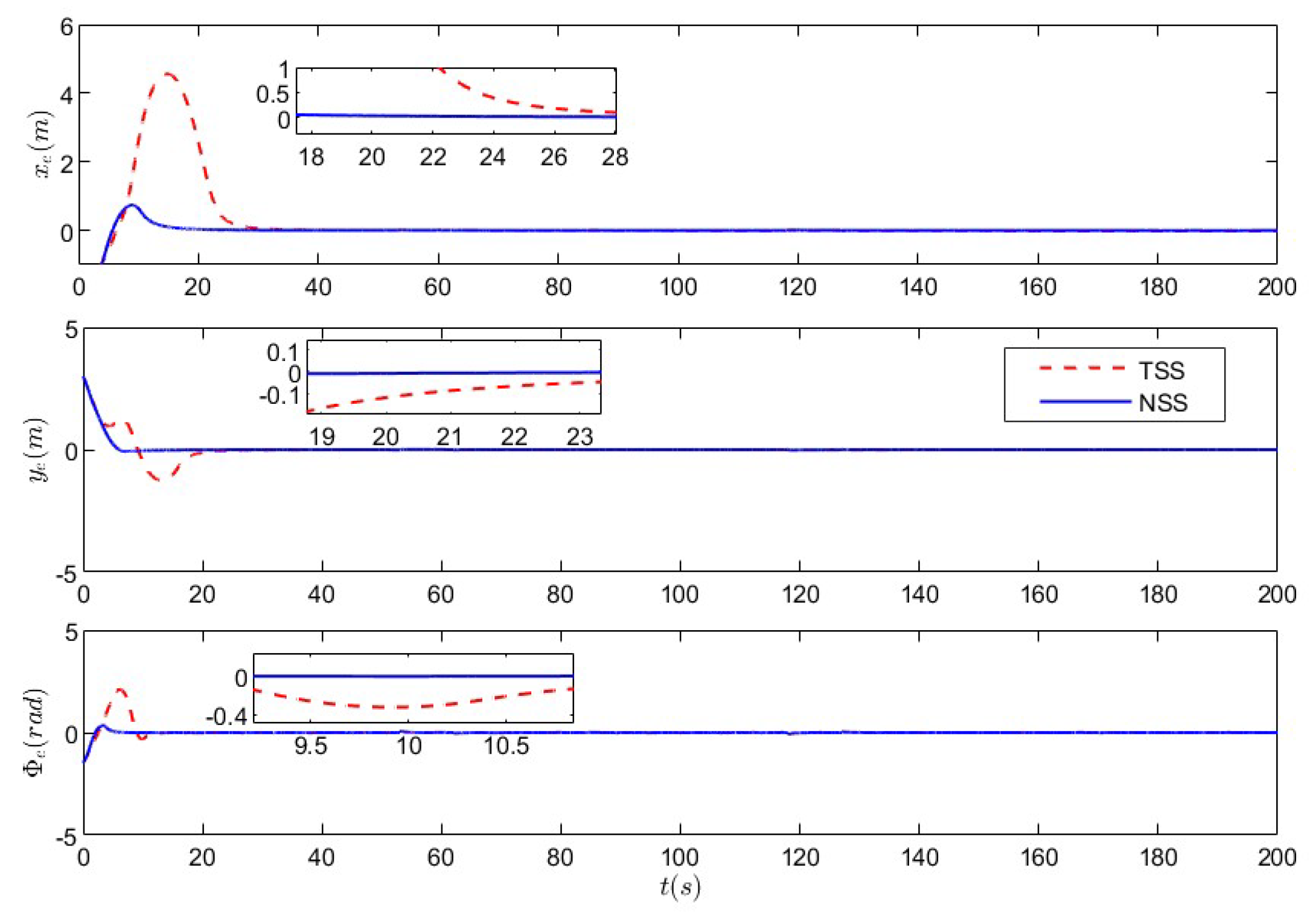
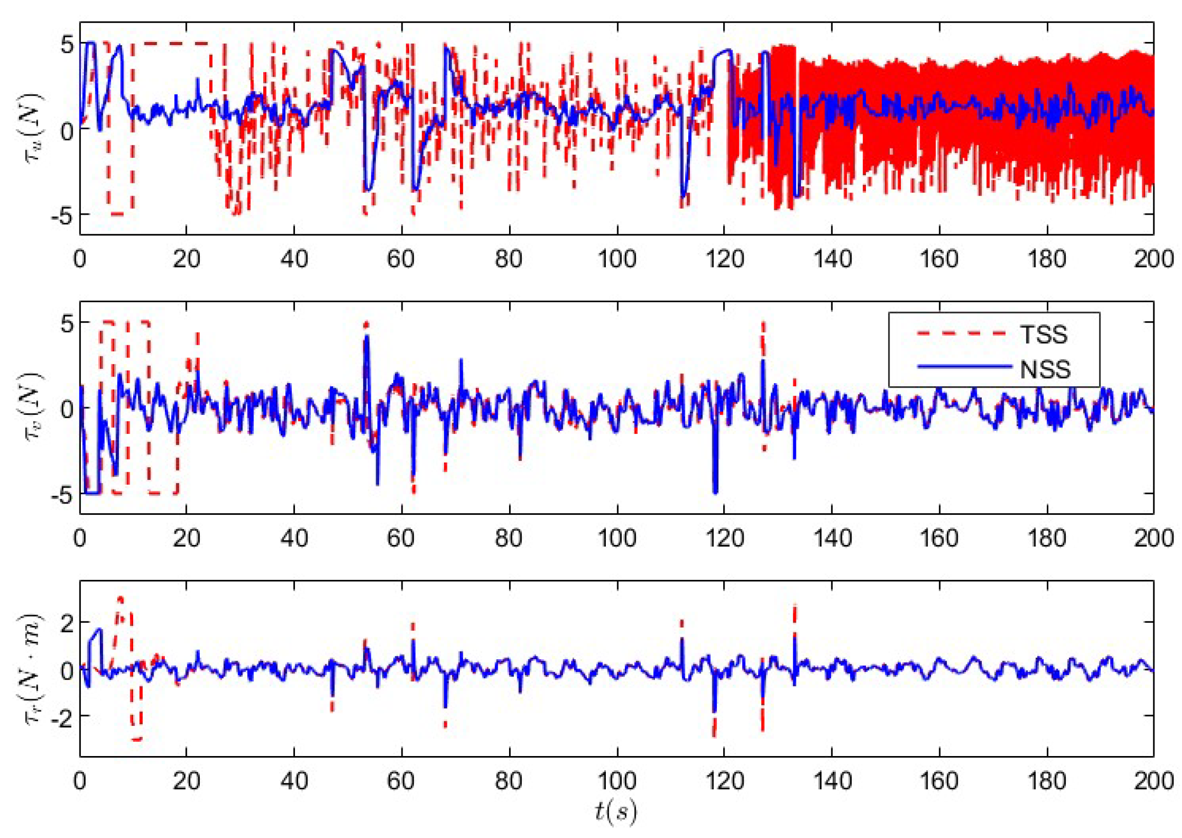
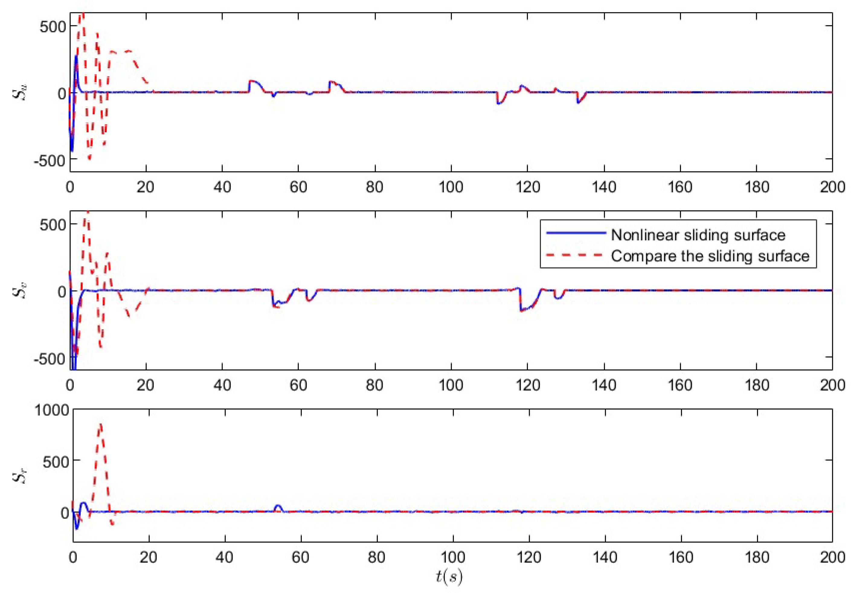
5.1. Nonlinear Sliding-Mode Super-Twisting Reaching Law Control Under Non-Deception Attack

To verify the applicability and effectiveness of the improved super-twisting reaching law algorithm in formation control, the interference resistance performance of a multi-ship formation system under non-deception attack conditions is first verified. The control law and adaptive law are given by Equations (58)–(60):

$${\tau }_{i3}\left(k\right)=-{\left({\gamma }_{ia}{\tau }_{max}\tilde{B}\right)}^{-1}{G}_{ic}{\dot{S}}_{ir}+{\gamma }_{ia}{\dot{u}}_{id}$$

(58)

$$\begin{array}{c}\hfill {\tau }_{i4}\left(k\right)=-{\left({\gamma }_{ia}{\tau }_{max}\tilde{B}\right)}^{-1}\left({\displaystyle \frac{1}{4r_{is}}}tanh\left({\displaystyle \frac{S_{iR}}{D}}\right)+r_{is}{r}_{i\Theta }{S}_{iR}{\phi }^4\left(Z_{iR}\right)\right){\widehat{\Theta }}_{iR}\end{array}$$

(59)

$$\begin{array}{c}\hfill {\dot{\widehat{\Theta }}}_{i2}={\displaystyle \frac{1}{4r_{is}}}tanh\left({\displaystyle \frac{S_{iR}}{D}}\right)S_{iR}-b{\widehat{\Theta }}_{iR}+r_{is}{r}_{i\Theta }{\parallel S_{iR}\parallel }^2{\phi }^4\left(Z_{iR}\right)\end{array}$$

(60)

Firstly, a simulation analysis and verification of the improved super-twisting reaching law control algorithm for the multi-ship formation system not attacked by random deception are carried out. The USV is subjected to an uncertain disturbance of ${\tau }_{id}=[{\tau }_{idu},{\tau }_{idv},{\tau }_{idr}]$, ${\tau }_{idu}=0.2sin(0.5t+\pi /4)$ N, ${\tau }_{idv}=0.18sin(0.5\ast t)+0.1cos\left(t\right)($N·m), and ${\tau }_{idr}=0.25cos\left(t\right)$ N. The total simulation time is 200 s and the step size is 0.01 s. In the simulation experiment, the initial position of the leader ship is $q_a\left(0\right)=[3,6,85\ast {180}^{-1}\pi ]$, the initial position of follow ship 1 is $q_{b1}\left(0\right)=[3,11,85\ast {180}^{-1}\pi ]$, and the initial position of follow ship 2 is $q_{b2}\left(0\right)=[4,5,85\ast {180}^{-1}\pi ]$.

In order to verify the effectiveness of the controller designed in this paper, the nonlinear sliding surface combined with an adaptive sliding reaching law is used as a comparison algorithm [43]. The kinematic parameters of the formation controller are ${\alpha }_1=diag(0.58,1.5,0.1)$, ${\alpha }_2=diag(0.6,1.5,0.1)$, and ${\alpha }_3=diag(0.7,1.5,0.9)$. The relevant parameters of the dynamic control sliding-mode surface are $a_u=diag(215,0.0001,0.1,10)$, $a_v=diag(215,0.0002,0.005,10)$, and $a_r=diag(210,0.0000085,0.05,20)$. The relevant parameters of the reaching law are $b_u=diag(0.0001,100)$, $b_v=diag(0.0015,185)$, and $b_r=diag(55,0.0052)$. The relevant parameters of the adaptive law are $c_u=diag(0.0001\times {10}^{-7},30)$, $c_v=diag(0.0001\times {10}^{-7},10)$, and $c_r=diag(0.0005\times {10}^{-2},10)$. The relevant parameters of the control law are $d_u=diag(1,0.0001,0.0001\times {10}^{-5})$, $d_v=diag(1,0.00001,0.00001)$, and $d_r=diag(1,0.00005,0.00005)$.

Figure 4 shows the multi-ship formation trajectory curves under the control algorithm designed in this paper. The nonlinear sliding-mode super-twisting reaching law control algorithm designed in this paper can make the leader ship and each follower ship form the formation more quickly while not under a deception attack and maintain the desired formation during the simulation time.

Figure 5, Figure 6 and Figure 7 show the position error simulation comparison of the leader ship and each follower ship while not under deception attack. It can be observed that using the controller designed in this paper, both the leader ship and each follower ship achieve stability within 20 s. The controller designed in this paper demonstrates better stability maintenance effects.

Figure 8, Figure 9 and Figure 10 give the system input curves for the leader ship and each follower ship under non-deception attacks. When the formation system is disturbed by uncertain disturbances, it causes abnormal inputs to the controller, and violent fluctuations are generated in the simulation figure. Comparing Figure 8, Figure 9 and Figure 10, it can be seen that the improved super-twisting reaching law proposed in this paper effectively enhances the dynamic acceleration characteristics of the sliding-mode reaching law, effectively suppressing the chattering phenomenon caused by the acceleration characteristics of the reaching law. Therefore, the system input under the control algorithm proposed in this paper can still maintain a small jitter amplitude when disturbed, which is beneficial for the control system when it comes to achieving better control performance.

Figure 11, Figure 12 and Figure 13 show that when the compare sliding surface changes, the influence of nonlinear terms near the sliding surface suddenly increases significantly. The system response changes, and the system chatter also undergoes significant changes. The improved sliding surface compensates for the integral saturation mechanism of the compare sliding surface. This reduces the sharp changes in the curvature of the sliding surface, significantly alleviating the chatter phenomenon on the sliding surface.

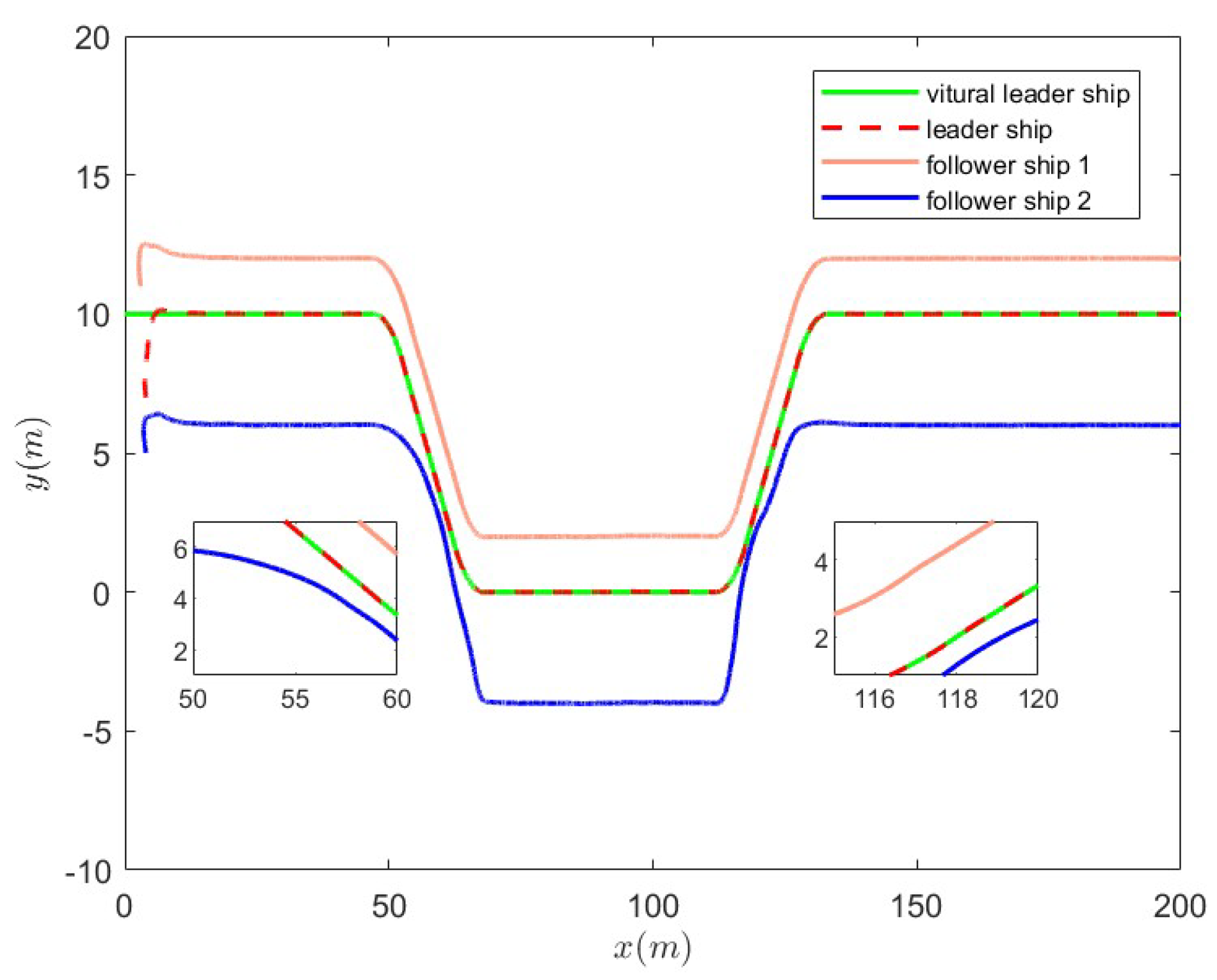
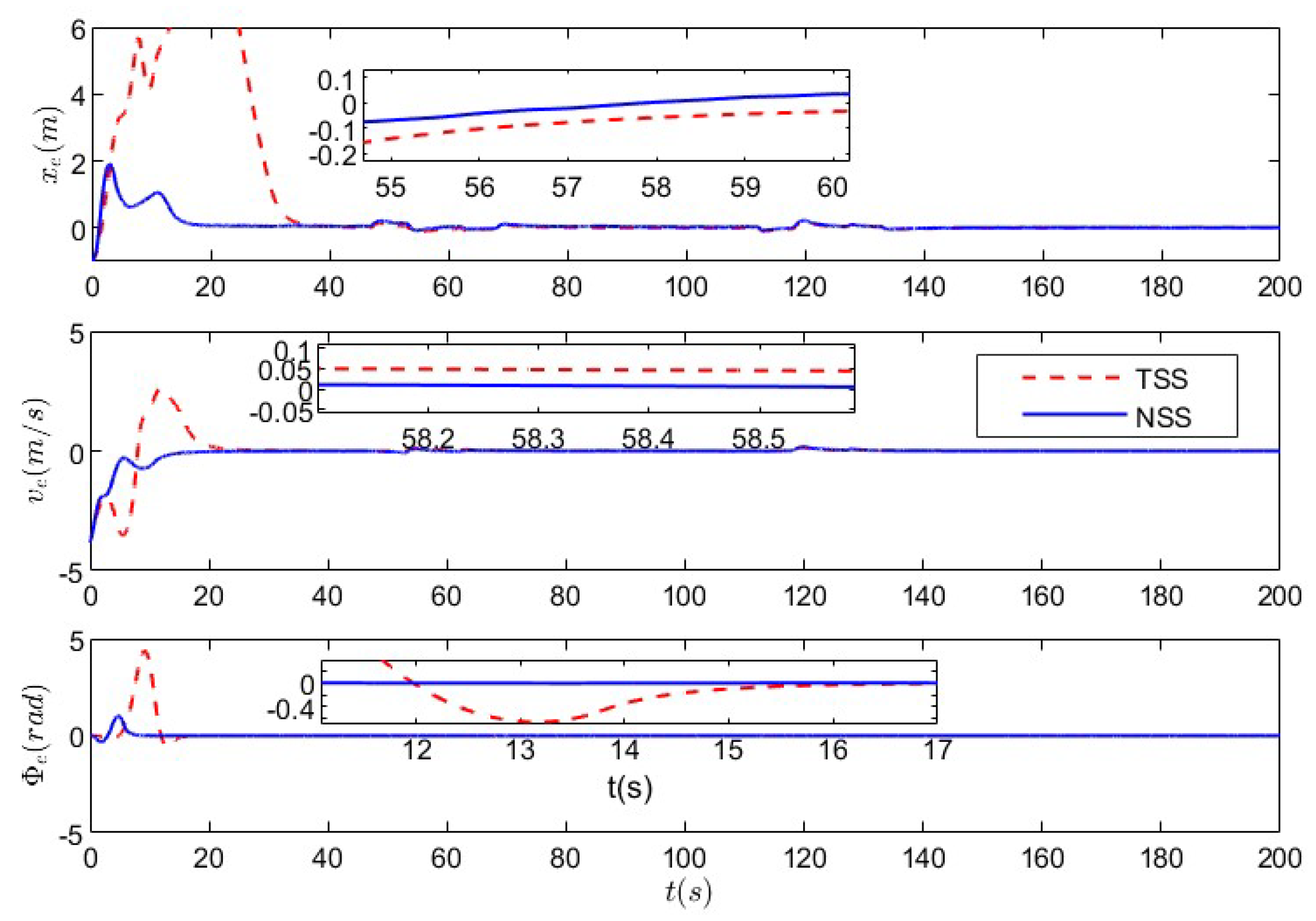
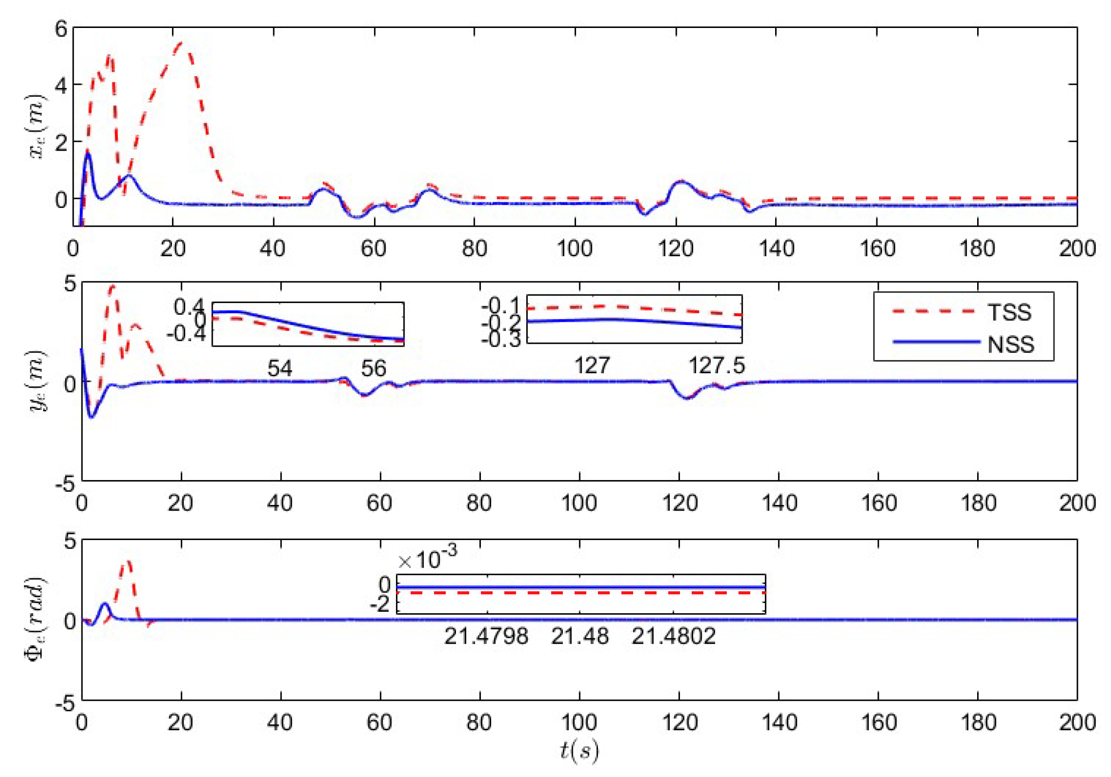
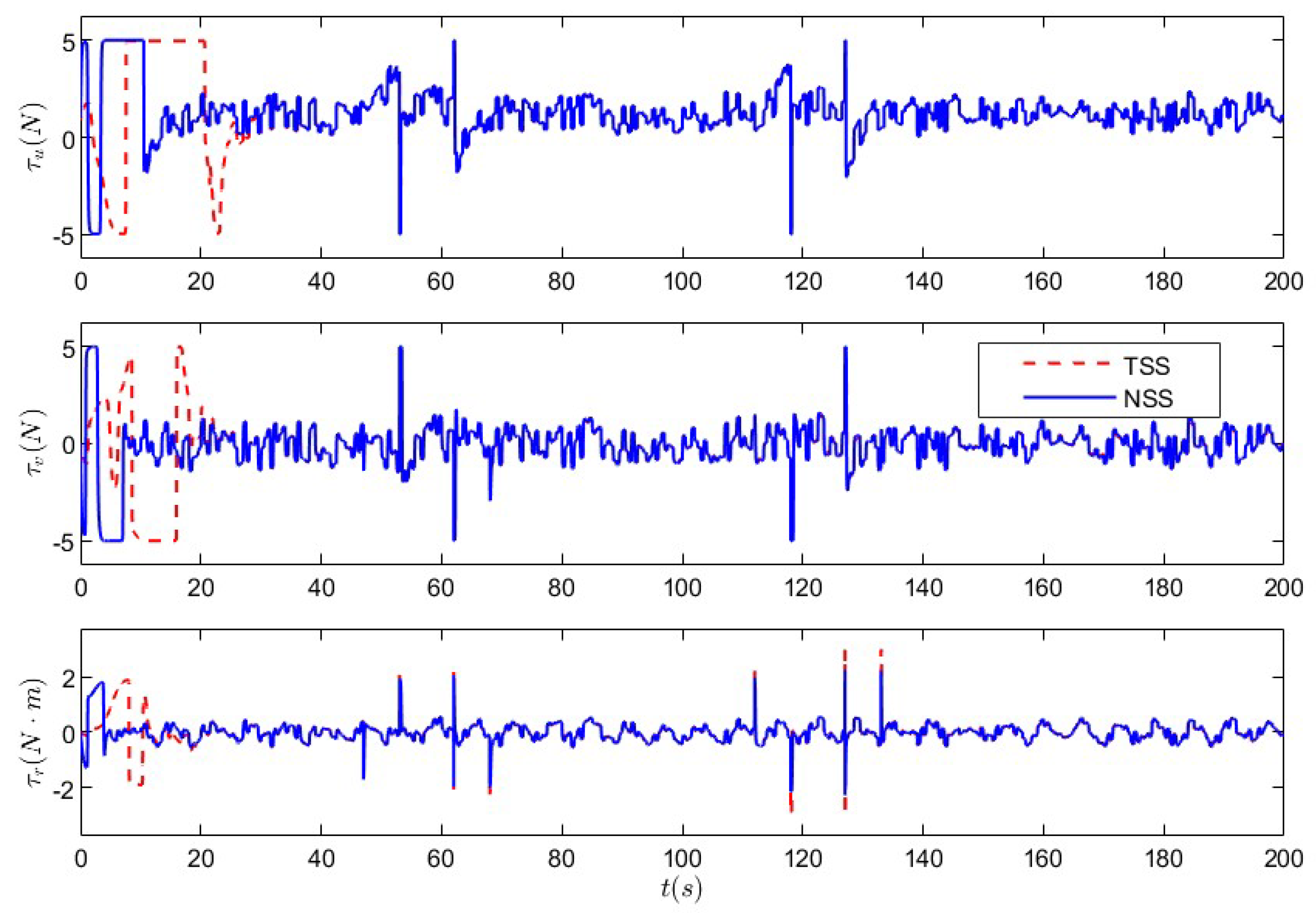
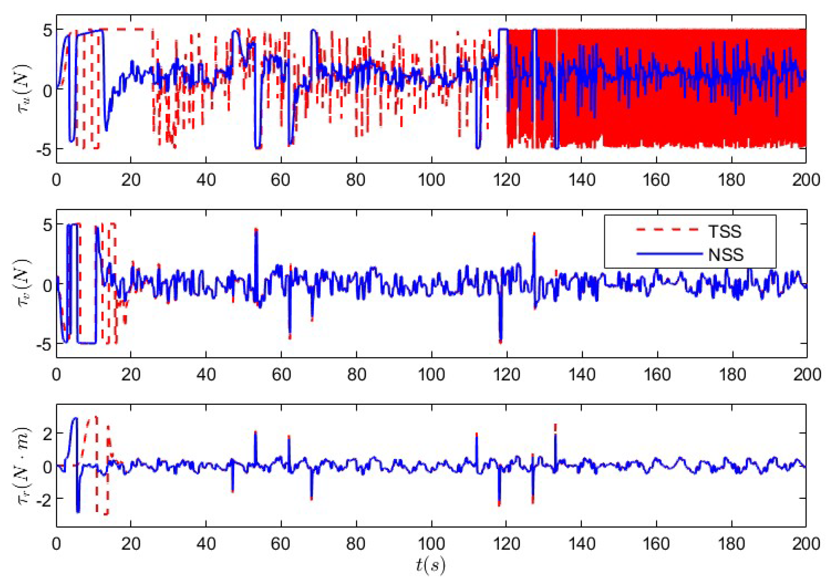
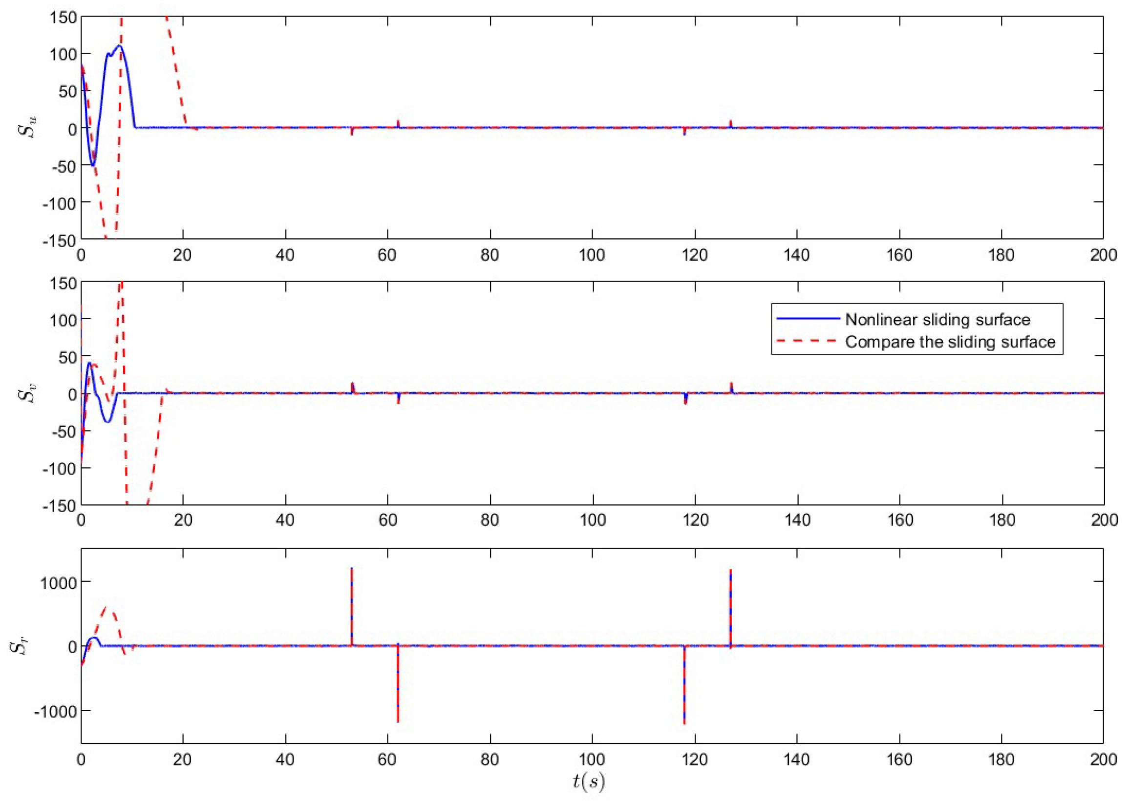
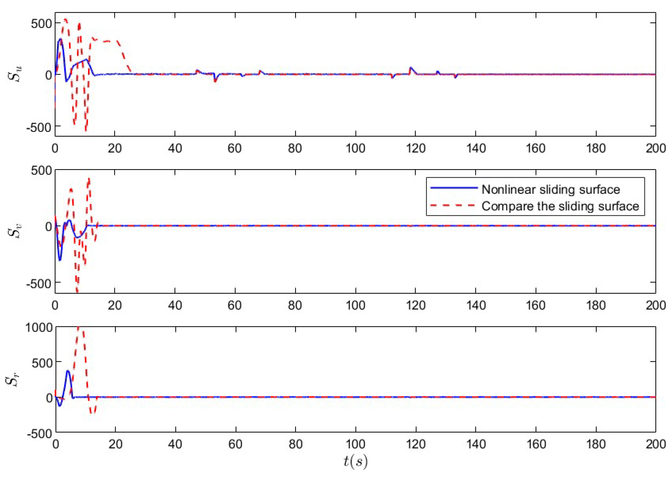
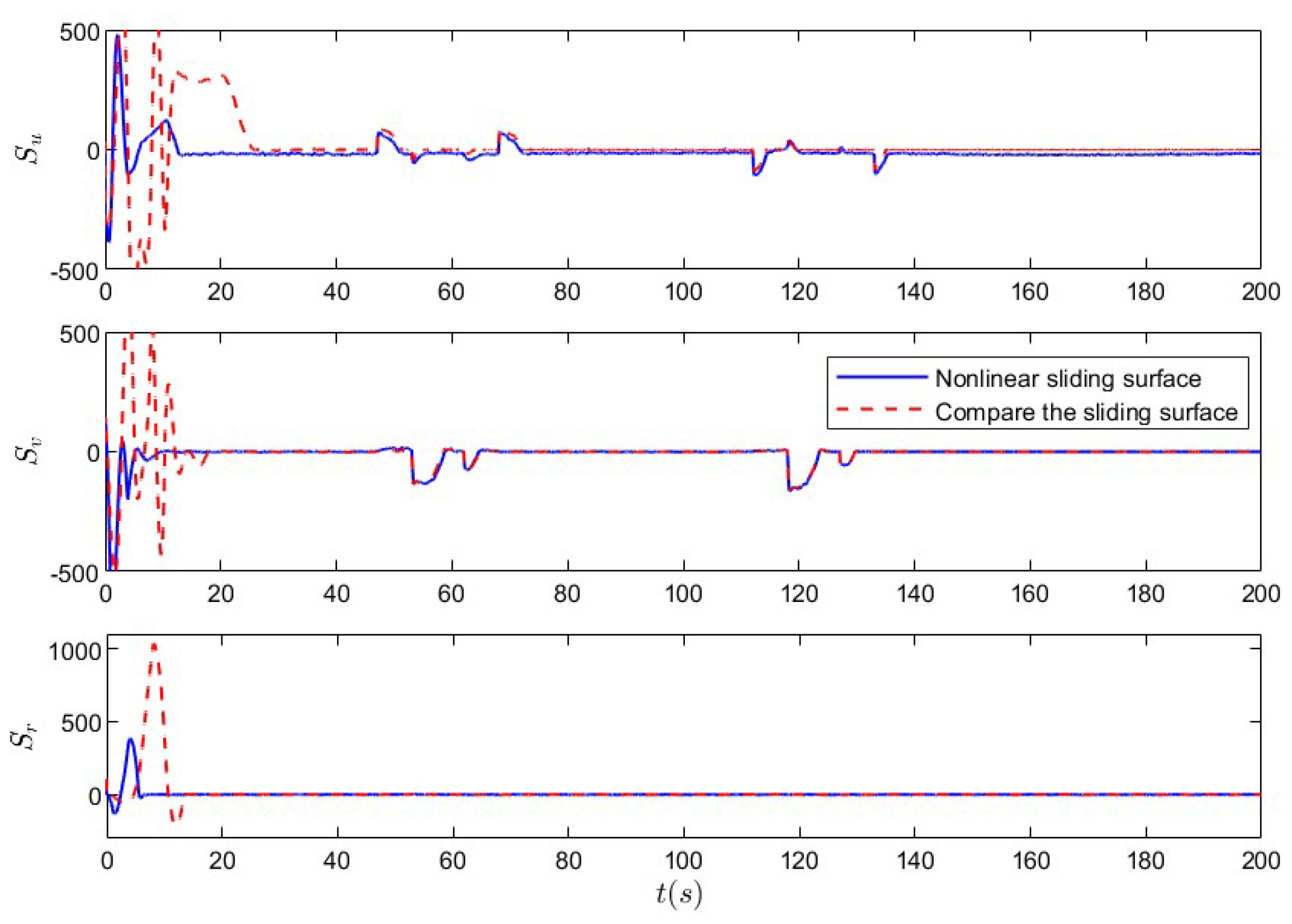
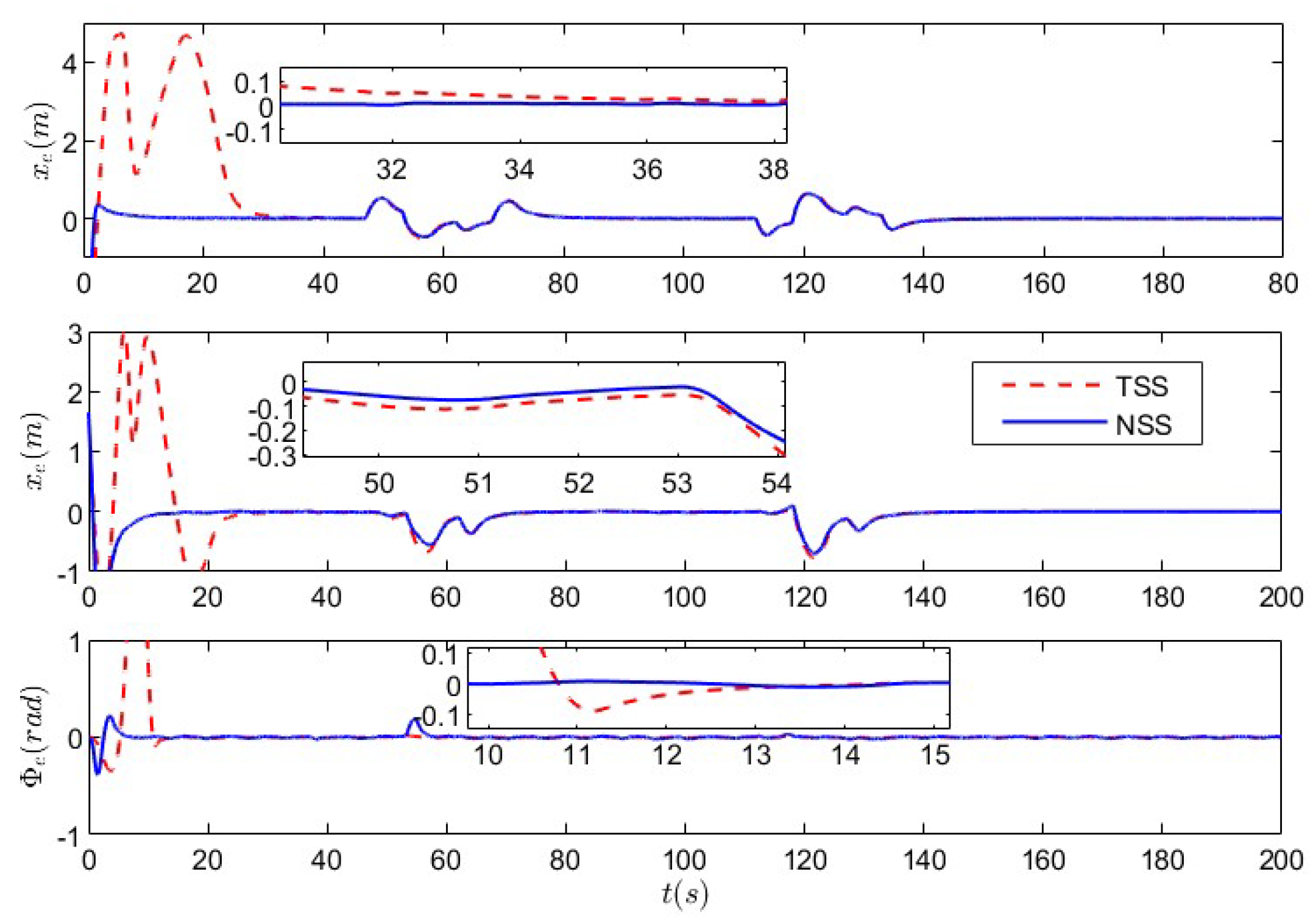
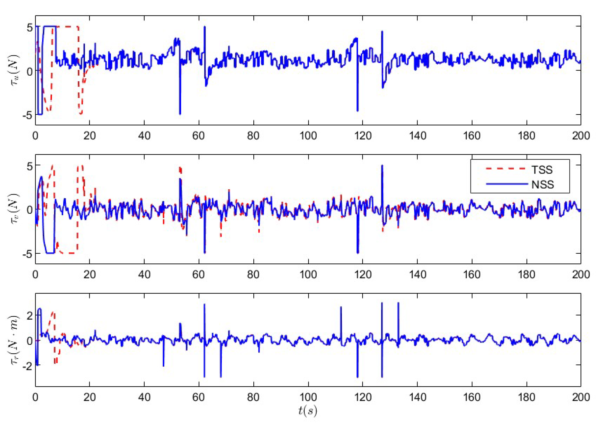
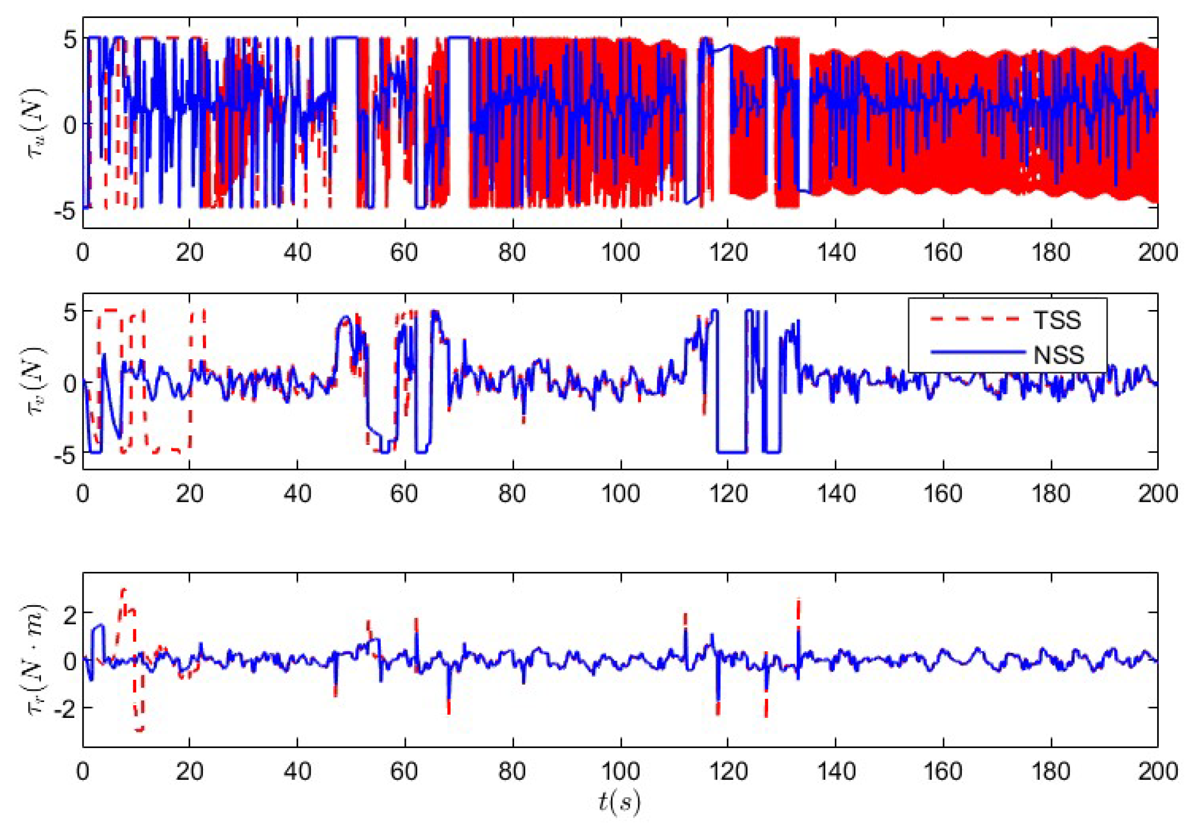
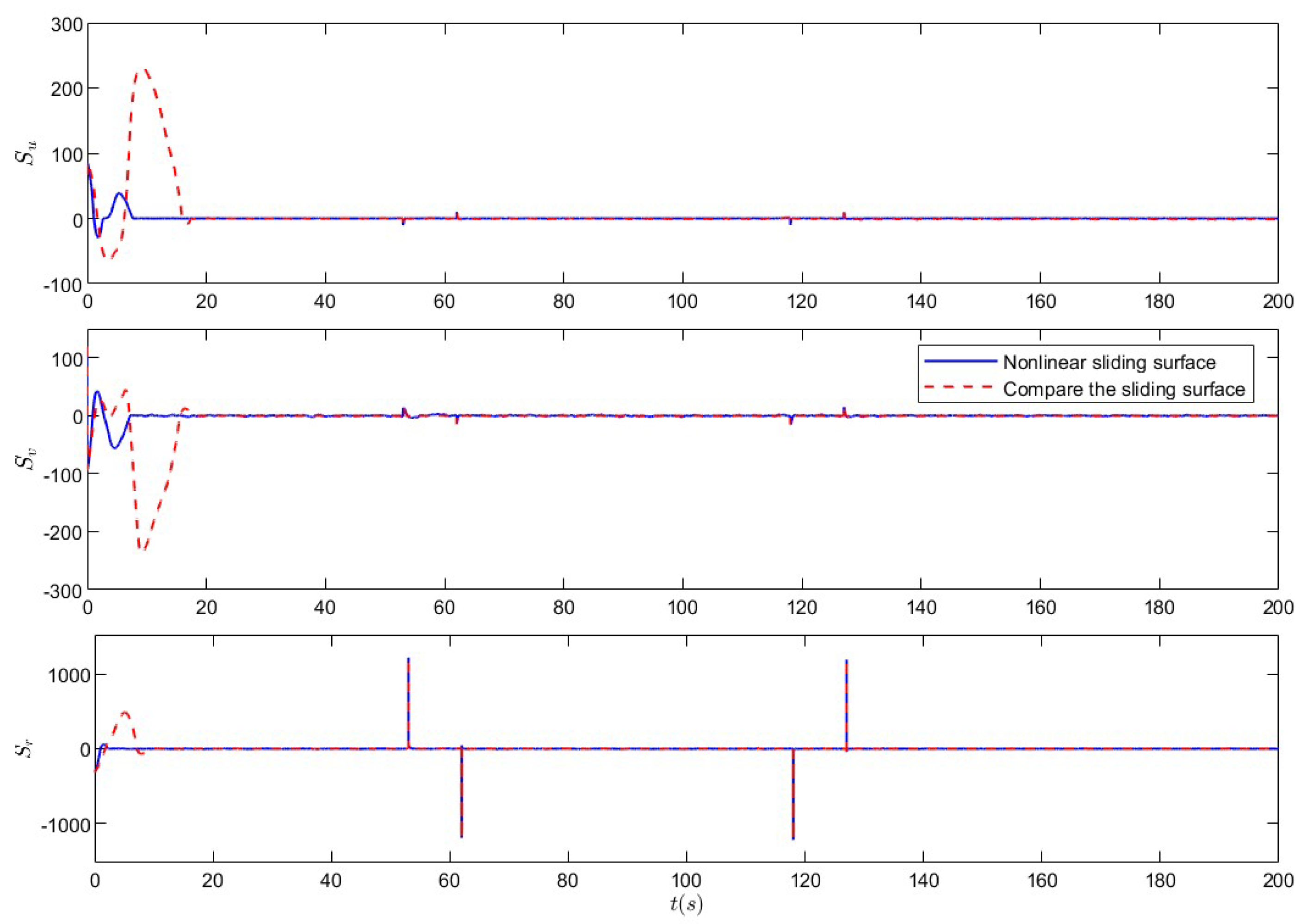
5.2. Nonlinear Sliding-Mode Super-Twisting Reaching Law Control Under Coupled Deception Attack

The above simulation results verify the effectiveness of the improved reaching law algorithm when multi-ships are not subjected to coupled deception attacks. In order to further verify the invasion resistance of the improved algorithm in the case of coupled attacks on the formation, Figure 14, Figure 15, Figure 16, Figure 17, Figure 18, Figure 19 and Figure 20 show a simulation comparison of USV formations under coupling deception attacks. The USV is subjected to an uncertain disturbance of ${\tau }_{id}=[{\tau }_{idu},{\tau }_{idv},{\tau }_{idr}]$, ${\tau }_{idu}=0.2sin(0.5t+\pi /4)$ N, ${\tau }_{idv}=0.18sin(0.5\ast t)+0.1cos\left(t\right)($N·m), and ${\tau }_{idr}=0.25cos\left(t\right)$ N. The total simulation time is 200 s and the step size is 0.01 s. In the simulation experiment, the initial position of the leader ship is $q_a\left(0\right)=[4,7,85\ast {180}^{-1}\pi ]$, the initial position of follow ship 1 is $q_{b1}\left(0\right)=[3,11,85\ast {180}^{-1}\pi ]$, and the initial position of follow ship 2 is $q_{b2}\left(0\right)=[4,5,85\ast {180}^{-1}\pi ]$.

In order to verify the effectiveness of the controller designed in this paper, the nonlinear sliding surface combined with an adaptive sliding reaching law is used as a comparison algorithm [43]. Deception attacks have a 35% attack probability; $A_{\zeta }\in [-2,2]$ is the random tampering interval of deception attacks. The kinematic parameters of the formation controller are ${\alpha }_1=diag(0.58,1.5,0.1)$, ${\alpha }_2=diag(0.6,1.5,0.1)$, and ${\alpha }_3=diag(0.7,1.5,0.9)$. The relevant parameters of the dynamic control sliding-mode surface are $a_u=diag(215,0.0001,0.1,10)$, $a_v=diag(215,0.0002,0.005,10)$, and $a_r=diag(210,0.0000085,0.05,20)$. The relevant parameters of the reaching law are $b_u=diag(0.0001,100)$, $b_v=diag(0.0015,185)$, and $b_r=diag(55,0.0052)$. The relevant parameters of the adaptive law are $c_u=diag(0.0001\times {10}^{-7},30)$, $c_v=diag(0.0001\times {10}^{-7},10)$, and $c_r=diag(0.0005\times {10}^{-2},10)$. The relevant parameters of the control law are $d_u=diag(1,0.0001,0.0001\times {10}^{-5})$, $d_v=diag(1,0.00001,0.00001)$, and $d_r=diag(1,0.00005,0.00005)$.

Figure 14 shows the formation trajectories of the leader ship and the follower ships in the formation system when subjected to coupling deceptive attacks and actuator physical fault coupling interference. It can be observed from the figure that the formation shape maintained under the super-twisting reaching law algorithm designed in this paper was not affected by the deceptive attacks and actuator physical fault coupling interference. In contrast to Figure 4, the trajectories of each single ship in the formation system only exhibited slight changes during the initial time frame, and under the influence of the controller, they quickly formed the desired formation and maintained the formation effect.

Figure 15, Figure 16 and Figure 17 show the position tracking errors in all directions of the leader ship and follower ships under deceptive attacks and actuator physical fault coupling interference, indicating that the comparison scheme reaches an error stabilization state relatively slowly and experiences significant fluctuations during the initial simulation time.

Table 1. The earliest convergence time of the position error of a single ship in the formation system.

	${\mathit{x}}_{\mathit{e}}$	Improvement Rate	${\mathit{y}}_{\mathit{e}}$	Improvement Rate	${\mathit{\varphi }}_{\mathit{e}}$	Improvement Rate
Leader ship	7 s	72%	8 s	70.4%	2 s	80.0%
Comparison leader ship	25 s		27 s		10 s
Follower ship 1	12 s	64.7%	12 s	55.6%	5 s	64.3%
Comparison follower ship 1	34 s		27 s		14 s
Follower ship 2	8 s	76.5%	12 s	55.6%	6 s	53.8%
Comparison follower ship 2	34 s		27 s		13 s

shows the earliest convergence time of the position error of a single ship in the formation system, demonstrating that all intelligent ships’ position tracking errors can stabilize within 12 s with the control scheme designed in this paper.

Figure 18, Figure 19 and Figure 20 show the system inputs of the leader ship and follower ship under random deceptive attack interference, indicating that under the control scheme designed in this paper, the system inputs are relatively stable under random attack interference conditions, which will significantly reduce the waste of communication resources caused by abnormal control inputs and also ensure the safety of the control process, facilitating the achievement of control objectives.

Figure 21, Figure 22 and Figure 23 show that under the coupled deception attack, the improved sliding surface can effectively mitigate the impact of nonlinear terms, preventing significant jitter in response to random deception attacks on the system. In contrast, the sliding surface exhibits severe jitter. The above simulation analysis demonstrates that the improved sliding control algorithm proposed in this paper has good control capabilities, effectively limiting system redundant errors within a finite range and improving the physical information saturation characteristics of the system. It not only provides robust resistance to uncertain disturbances for formation systems but also resists interference from random deception attacks.

6. Conclusions

This paper studies a USV formation system where abnormal inputs are generated by deception attacks and physical failures of actuators, and designs an improved nonlinear sliding-mode super-twisting reaching law control algorithm. First, considering the reaching phase of the sliding surface, to reduce system-induced chattering issues, improve abnormal inputs, and enhance the reaching efficiency of the sliding-mode surface, a nonlinear damping and super-twisting reaching law is designed to improve the robust response efficiency of systems. Simulation results verify that this formation system not only maintains its overall shape but also improves the control accuracy of each vessel, with the earliest convergence time for position errors of individual vessels increasing by at least 50%, effectively enhancing the collaborative mining operation efficiency of USV-ROV systems in practical applications. However, the simulation experiment has certain limitations. Future research can supplement the existing simulation results by combining them with experimental data from actual scenarios to further verify our method.

References

1. Bai, X.E.; Li, B.H.; Xu, X.F.; Xiao, Y.J. A review of current research and advances in unmanned surface vehicles. J. Mar. Sci. Appl. 2022, 21, 47–58. [Google Scholar] [CrossRef]
2. Khanmeh, J.; Wanderlingh, F.; Indiveri, G.; Simetti, E. Design and Control of a Cooperative System of an Autonomous Surface Vehicle and a Remotely Operated Vehicle (ASV-ROV). In Proceedings of the 2024 20th IEEE/ASME International Conference on Mechatronic and Embedded Systems and Applications (MESA), Genova, Italy, 2–4 September 2024; pp. 1–7. [Google Scholar]
3. Qiao, Y.; Yin, J.; Wang, W.; Duarte, F.; Yang, J.; Ratti, C. Survey of Deep Learning for Autonomous Surface Vehicles in Marine Environments. IEEE Trans. Intell. Transp. Syst. 2023, 24, 3678–3701. [Google Scholar] [CrossRef]
4. Zhao, C.; Thies, P.R.; Johanning, L. Investigating the winch performance in an ASV/ROV autonomous inspection system. Appl. Ocean. Res. 2021, 115, 102827. [Google Scholar] [CrossRef]
5. Du, J.; Jiang, B.; Jiang, C.; Shi, Y.; Han, Z. Gradient and channel aware dynamic scheduling for over-the-air computation in federated edge learning systems. IEEE J. Sel. Areas Commun. 2023, 41, 1035–1050. [Google Scholar] [CrossRef]
6. Ding, L.; Guo, G. Formation control for ship fleet based on backstepping. Control Decis. 2012, 27, 299–303. [Google Scholar]
7. Lu, Y.; Zhang, G.; Sun, Z.; Zhang, W. Adaptive cooperative formation control of autonomous surface vessels with uncertain dynamics and external disturbances. Ocean Eng. 2018, 167, 36–44. [Google Scholar] [CrossRef]
8. Lin, A.; Jiang, D.; Zeng, J. Underactuated ship formation control with input saturation. Acta Autom. Sin. 2018, 33, 1496–1504. [Google Scholar]
9. Van, M. An enhanced tracking control of marine surface vessels based on adaptive integral sliding-mode control and disturbance observer. ISE Trans. 2019, 90, 30–40. [Google Scholar] [CrossRef]
10. Martin, S.C.; Whitcomb, L.L. Nonlinear model-based tracking control of underwater vehicles with three degree-of-freedom fully coupled dynamical plant models: Theory and experimental evaluation. IEEE Trans. Control Syst. Technol. 2018, 26, 404–414. [Google Scholar] [CrossRef]
11. Ma, Y.; Qi, X.; Li, Z.; Hu, S.; Sotelo, M.Á. Resilient Control for Networked Unmanned Surface Vehicles With Dynamic Event-Triggered Mechanism Under Aperiodic DoS Attacks. IEEE Trans. Veh. Technol. 2024, 73, 5824–5833. [Google Scholar] [CrossRef]
12. Li, M.; Yu, C.; Zhang, X.; Liu, C.; Lian, L. Fuzzy adaptive trajectory tracking control of work-class ROVs considering thruster dynamics. Ocean Eng. 2024, 267, 113232. [Google Scholar] [CrossRef]
13. Li, T.; Zhao, R.; Chen, C.L.P.; Fang, L.; Liu, C. Finite-Time Formation Control of Under-Actuated Ships Using Nonlinear sliding-mode Control. IEEE Trans. Cybern. 2018, 48, 3243–3253. [Google Scholar] [CrossRef] [PubMed]
14. Chen, Z.; Zhang, Y.; Zhang, Y.; Nie, Y.; Tang, J.; Zhu, S. Disturbance-observer-based sliding-mode control design for nonlinear unmanned surface vessel with uncertainties. IEEE Access 2019, 7, 148522–148530. [Google Scholar] [CrossRef]
15. Yang, M.; Sheng, Z.; Yin, G.; Wang, H. A recurrent neural network based fuzzy sliding-mode control for 4-DOF ROV movements. Ocean Eng. 2022, 256, 111509. [Google Scholar] [CrossRef]
16. Schauer, S.; Kalogeraki, E.M.; Papastergiou, S.; Douligeris, C. Detecting sophisticated attacks in maritime environments using hybrid situational awareness. In Proceedings of the 2019 International Conference on Information and Communication Technologies for Disaster Management (ICT-DM), Paris, France, 18–20 December 2019; pp. 1–7. [Google Scholar]
17. Li, S.; Cheng, X.; Shi, F.; Zhang, H.; Dai, H.; Zhang, H.; Chen, S. A novel robustness-enhancing adversarial defense approach to AI-powered sea state estimation for autonomous marine vessels. IEEE Trans. Syst. Man Cybern. Syst. 2024, 55, 28–42. [Google Scholar] [CrossRef]
18. Zhang, G.; Yao, M.; Xu, J.; Zhang, W. Robust neural event-triggered control for dynamic positioning ships with actuator faults. Ocean Eng. 2020, 207, 107292. [Google Scholar] [CrossRef]
19. Hu, S.; Chen, X.; Li, J.; Xie, X. Observer-Based Resilient Controller Design for Networked Stochastic Systems Under Coordinated DoS and FDI Attacks. IEEE Trans. Control. Netw. Syst. 2024, 11, 890–901. [Google Scholar] [CrossRef]
20. Zhao, Y.; Qi, X.; Ma, Y.; Li, Z.; Malekian, R.; Sotelo, M.A. Path Following Optimization for an Underactuated USV Using Smoothly-Convergent Deep Reinforcement Learning. IEEE Trans. Intell. Transp. Syst. 2021, 22, 6208–6220. [Google Scholar] [CrossRef]
21. Erbas, M.; Khalil, S.M.; Tsiopoulos, L. Systematic literature review of threat modeling and risk assessment in ship cybersecurity. Ocean Eng. 2024, 306, 118059. [Google Scholar] [CrossRef]
22. Tam, K.; Hopcraft, R.; Moara-Nkwe, K.; Misas, J.P.; Andrews, W.; Harish, A.V.; Giménez, P.; Crichton, T.; Jones, K. Case study of a cyber-physical attack affecting port and ship operational safety. J. Transp. Technol. 2021, 12, 1–27. [Google Scholar] [CrossRef]
23. Bhatti, J.; Humphreys, T.E. Hostile control of ships via false GPS signals: Demonstration and detection. Navig. J. Inst. Navig. 2017, 64, 51–66. [Google Scholar] [CrossRef]
24. Gao, S.; Peng, Z.; Liu, L.; Wang, D.; Han, Q.-L. Fixed-time resilient edge-triggered estimation and control of surface vehicles for cooperative target tracking under attacks. IEEE Trans. Intell. 2023, 8, 547–556. [Google Scholar] [CrossRef]
25. Mahmoud, M.S.; Hamdan, M.M.; Baroudi, U.A. Modeling and control of cyber-physical systems subject to cyber attacks: A survey of recent advances and challenges. Neurocomputing 2019, 338, 101–115. [Google Scholar] [CrossRef]
26. Ubaleht, J. Importance of Positioning to MASS: The Effect of Jamming and Spoofing on Autonomous Vessel. Master’s Thesis, University of Turku, Turku, Finland, 2022. [Google Scholar]
27. Elsisi, M.; Yu, J.T.; Lai, C.C.; Su, C.L. A drone-assisted deep learning based IoT system for monitoring ship emissions in ports considering adversarial attacks. IEEE Trans. Instrum. Meas. 2024, 73, 9506111. [Google Scholar] [CrossRef]
28. Vagale, A.; Oucheikh, R.; Bye, R.T.; Osen, O.L.; Fossen, T.I. Path planning and collision avoidance for autonomous surface vehicles I: A review. J. Mar. Sci. Technol. 2021, 26, 1292–1306. [Google Scholar] [CrossRef]
29. Ohn, S.W.; Namgung, H. Requirements for optimal local route planning of autonomous ships. J. Mar. Sci. Eng. 2022, 11, 17. [Google Scholar] [CrossRef]
30. Namgung, H.; Kim, J.S. Collision risk inference system for maritime autonomous surface ships using COLREGs rules compliant collision avoidance. IEEE Access 2021, 9, 7823–7835. [Google Scholar] [CrossRef]
31. Chen, X.; Jia, T.; Wang, Z.; Xie, X.; Qiu, J. Practical fixed-time bipartite synchronization of uncertain coupled neural networks subject to deception attacks via dual-channel event-triggered control. IEEE Trans. Cybern. 2023, 54, 3615–3625. [Google Scholar] [CrossRef]
32. Yang, W.; Shi, Z.; Zhong, Y. Robust time-varying formation control for uncertain multi-agent systems with communication delays and nonlinear couplings. Int. J. Robust Nonlinear Control. 2024, 34, 147–166. [Google Scholar] [CrossRef]
33. Zhang, C.; Yu, S. Disturbance observer-based prescribed performance super-twisting sliding-mode control for autonomous surface vessels. ISA Trans. 2023, 135, 13–22. [Google Scholar] [CrossRef]
34. Feng, C.; Chen, W.; Tao, R.; Zhu, D.; Chu, K. Adaptive Super-Spiral Trajectory Tracking sliding-mode Control for Unmanned Vessels. Electron. Meas. Technol. 2024, 47, 37–44. [Google Scholar]
35. Liu, W.; Du, J.; Li, J.; Li, Z. Robust Control of Shipborne Stable Platforms Based on Hyperhelix Slip Mode. Syst. Eng. Electron. Technol. 2022, 44, 1662–1669. [Google Scholar]
36. Liu, Y.; Xu, C.; Zhao, Y.; Liu, S.; Liang, X. Tracking Control of Underdriven Vessels Based on Hyperhelical sliding-mode. Inf. Control. 2022, 49, 578–584, 597. [Google Scholar]
37. Sonnenburg, C.R.; Woolsey, C.A. Modeling. identification, and control of an unmanned surface vehicle. J. Field Robot. 2013, 30, 371–398. [Google Scholar] [CrossRef]
38. Dong, Z.; Qi, S.; Yu, M.; Zhang, Z.; Zhang, H.; Li, J.; Liu, Y. An improved dynamic surface sliding-mode method for autonomous cooperative formation control of underactuated USVs with complex marine environment disturbances. Pol. Marit. Res. 2022, 29, 47–60. [Google Scholar] [CrossRef]
39. Min, H.; Xu, S.; Zhang, Z. Adaptive finite-time stabilization of stochastic nonlinear systems subject to full-state constraints and input saturation. IEEE Trans. Autom. Control. 2020, 66, 1306–1313. [Google Scholar] [CrossRef]
40. Zhang, X.M.; Han, Q.L. Event-triggered dynamic output feedback control for networked control systems. IET Control Theory Appl. 2014, 8, 226–234. [Google Scholar] [CrossRef]
41. Fallaha, C.J.; Saad, M.; Kanaan, H.Y.; Al-Haddad, K. Sliding-Mode Robot Control With Exponential Reaching Law. IEEE Trans. Ind. Electron. 2011, 58, 600–610. [Google Scholar] [CrossRef]
42. Skjetne, R.; Fossen, T.I.; Kokotović, P.V. Adaptive maneuvering, with experiments, for a model ship in a marine control laboratory. Automatica 2005, 41, 289–298. [Google Scholar] [CrossRef]
43. Mobayen, S. Adaptive global sliding-mode control of underactuated systems using a super-twisting scheme: An experimental study. J. Vib. Control. 2019, 25, 2215–2224. [Google Scholar] [CrossRef]
Figure 1. Formation geometric coordinate system.
Jmse 13 00561 g001
Figure 2. Reaching law arrival velocity comparison.
Jmse 13 00561 g002
Figure 3. Reaching law acceleration gain comparison.
Jmse 13 00561 g003
Figure 4. Non-attack formation trajectory.
Jmse 13 00561 g004
Figure 5. Non-deception attack leader ship position error.
Jmse 13 00561 g005
Figure 6. Non-deception attack follow ship 1 position error.
Jmse 13 00561 g006
Figure 7. Non-deception attack follow ship 2 position error.
Jmse 13 00561 g007
Figure 8. Non-deception attack leader ship input error.
Jmse 13 00561 g008
Figure 9. Non-deception attack follow ship 1 input error.
Jmse 13 00561 g009
Figure 10. Non-deception attack follow ship 2 input error.
Jmse 13 00561 g010
Figure 11. Non-deception attack leader ship sliding surface.
Jmse 13 00561 g011
Figure 12. Non-deception attack follow ship 1 sliding surface.
Jmse 13 00561 g012
Figure 13. Non-deception attack follow ship 2 sliding surface.
Jmse 13 00561 g013
Figure 14. Formation trajectory under coupled attack interference.
Jmse 13 00561 g014
Figure 15. Position error of leader ship under coupled attack interference.
Jmse 13 00561 g015
Figure 16. Position error of the follow ship 1 under coupled attack interference.
Jmse 13 00561 g016
Figure 17. Position error of follow ship 2 under coupled attack interference.
Jmse 13 00561 g017
Figure 18. Input of leader ship under coupled attack interference.
Jmse 13 00561 g018
Figure 19. Input of follow ship 1 under coupled attack interference.
Jmse 13 00561 g019
Figure 20. Input of follow ship 2 under coupled attack interference.
Jmse 13 00561 g020
Figure 21. Leader ship sliding surface under coupled attack interference.
Jmse 13 00561 g021
Figure 22. Follow ship 1 sliding surface under coupled attack interference.
Jmse 13 00561 g022
Figure 23. Follow ship 2 sliding surface under coupled attack interference.
Jmse 13 00561 g023