A Low-Complexity Path-Planning Algorithm for Multiple USVs in Task Planning Based on the Visibility Graph Method

Abstract

Path planning for multiple unmanned surface vehicles (USVs) in task planning is a high-complexity problem. When the number of USVs is $n$, the computational complexity is usually as high as $O\left(n^2\right)$, as paths need to be planned from different start points to different target points. In this paper, we propose a low-complexity path-planning algorithm (LCPP) for multiple USVs based on the visibility graph method. First, all paths between the start points, target points, and obstacle vertices are separately planned with the low-complexity $O\left(n\right)$. After that, the Dijkstra algorithm is employed to find the shortest path from each start point to all target points, also with the low-complexity $O\left(n\right)$. To enhance the safety of each USV traveling along the edge of obstacles, the parameters of the adaptive line-of-sight (ALOS) guidance algorithm are optimized using the simulated annealing algorithm. The simulation results show that this algorithm outperforms others in calculation time when dealing with a large number of USVs.

1. Introduction

With the improvement and refinement of unmanned surface vehicle (USV) systems, the application of multiple USVs is gradually expanding in the tasks with increasing complexity and scale. The execution of tasks by multiple USVs is receiving more and more attention, such as monitoring pollutants [1], water quality detection [2], warehouse logistics [3], mapping [4], and hunting [5]. The path planning for multiple USVs is one of the important foundations and prerequisites for task planning and execution [6].

Recently, there has been progress regarding path planning for USVs in task planning. To reduce computational complexity, some researchers use the Euclidean Distance instead of path planning to construct the cost matrix for task planning, and plan paths after task allocation [7,8,9,10,11], while others study path-planning solutions that reduce complexity. Xia et al. [12] proposed an improved genetic algorithm with the shortest path for the path planning of the USV accessing the task nodes after multi-task assignment, and an artificial potential field function was proposed to avoid USV collision during navigation. Ma et al. [13] proposed the collaborative coverage-improved BA* algorithm (CCIBA*). In the algorithm, coverage path planning for a single vehicle is achieved by task decomposition and level map updating. Then, a multiple-vehicle collaborative behavior strategy was designed for coverage path planning, composed of area division, recall and transfer, area exchange, and recognizing obstacles. Zhao et al. [14] proposed a region division method based on a Voronoi diagram, which divides the region and assigns it to each USV. The improved salp swarm algorithm was used to solve the traditional model predictive control (MPC) for path planning. Yao et al. [15] used the bioinspired neural network to plan the standard path of a single USV for obstacle avoidance between the start point and destination. Then, based on the result of the neural activity values, the cost matrix of the Hungarian algorithm was built and modified for task assignment among multi-USVs. Yu et al. [16] proposed the improved Hungarian algorithm used for multi-target allocation and a virtual field RRT* algorithm to solve the problem of path planning for multi-USVs in space-varying ocean currents. Pei et al. [17] proposed an improved Dyna-Q algorithm incorporating heuristic search strategies, the simulated annealing mechanism, and the reactive navigation principle into Q-learning based on the Dyna architecture for robots in the grid map. A novel action-selection strategy combining the ε-greedy policy with the cooling schedule control is presented to tackle the exploration–exploitation dilemma and enhance the performance of global searching, the convergence property, and learning efficiency for path planning. Zhang et al. [18] proposed a new path-planning method that utilizes integrated environment representation and reinforcement learning to control a mobile robot with non-holonomic constraints in unknown dynamic environments. With the control algorithm presented, the novel approach enables one to find the optimal path to the target efficiently and avoid collisions without the shapes of the obstacles or even any information about the obstacles’ velocities. Wu et al. [19] proposed a novel deep neural network (DNN)-based method for real-time online path planning, including an online three-dimensional path planning network to learn 3D local path planning policies and a path planning framework to realize near-optimal real-time online path planning.

Most research focuses on reducing the complexity of path planning for single USVs. However, a large number of USVs and more possible allocation schemes result in a lot of paths that need to be planned with global centralized computing for large-scale and complex task planning. When the number of USVs is $n$, the computational complexity is usually as high as $O\left(n^2\right)$, as paths need to be planned from all different start points to all different target points. When the number of USVs is large, the calculation time of traditional path-planning algorithms will be too long. Therefore, the complexity of the path planning of multiple USVs needs to be reduced [20], as shown in

Table 1. Differences in path planning for multiple USVs in task planning.

	The Traditional Path-Planning Algorithms	A Low-Complexity Path Planning Algorithm
The planned path	Plan $n^2$ paths (from $n$ start points to $n$ target points).	Plan possible paths and find the shortest path
Computational complexity	$O\left(n^2\right)$	Plan possible paths: $O\left(n\right)$ Find the shortest paths: $O\left(n\right)$ (Obstacles are stationary and have a fixed number)
Calculation time	Exponential growth	Linear growth

.

The main contributions in this paper can be summarized as follows:

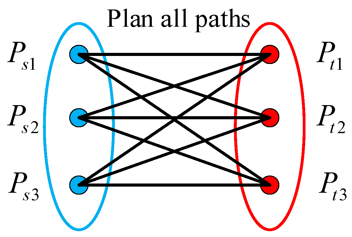
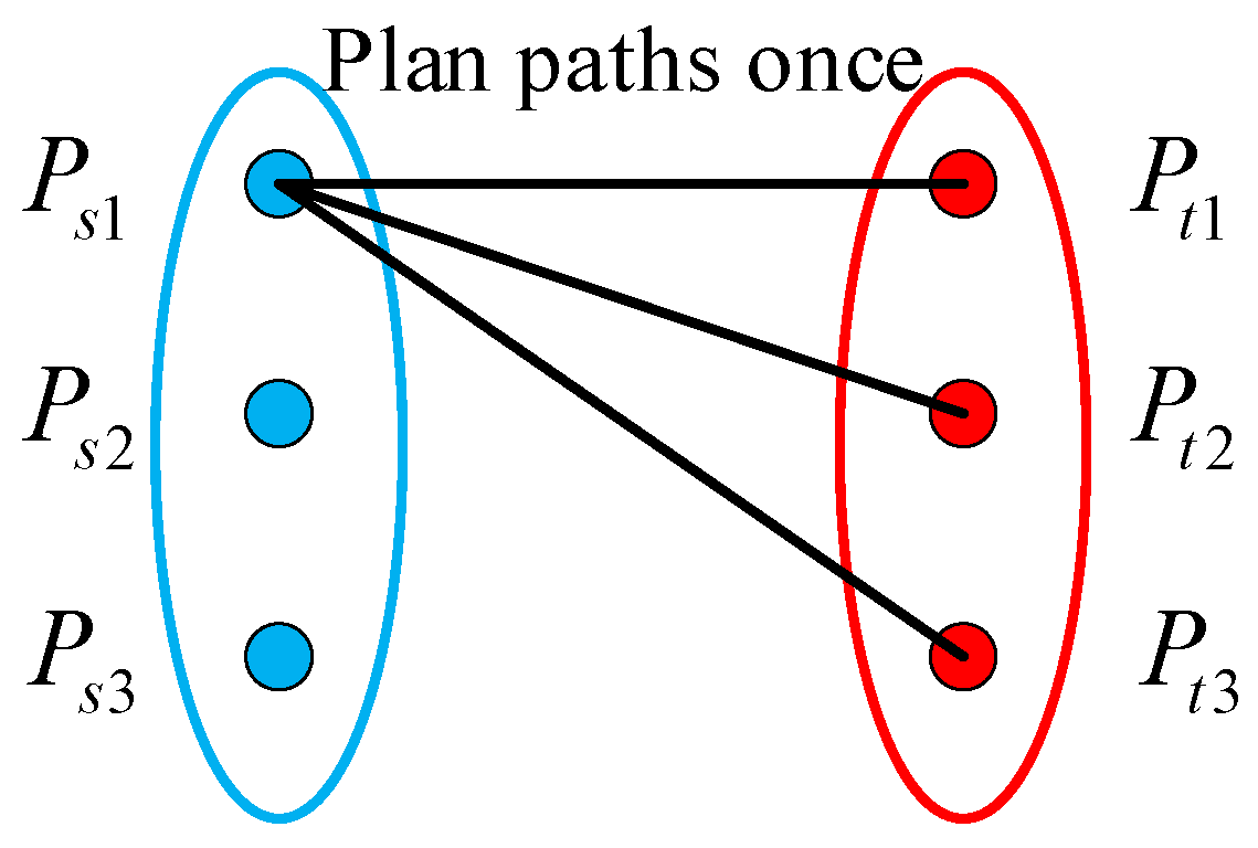
• A low-complexity path-planning algorithm (LCPP) for multiple USVs is proposed based on the visibility graph method, which reduces the computational complexity from $O\left(n^2\right)$ to $O\left(n\right)$.
• The parameters of the adaptive line-of-sight (ALOS) guidance algorithm are optimized using the simulated annealing algorithm to enhance the safety of each USV traveling along the edge of obstacles.

The remainder of this paper is organized as follows. Section 2 formulates and analyzes the path planning for multiple USVs in task planning. Section 3 presents the low-complexity path planning algorithm (LCPP) and ALOS with the optimized parameter. The results of simulation and comparison are presented in Section 4, followed by conclusions in Section 5.

2. Problem Modeling

The frequently used notations are shown in

Table 2. Frequently used notations.

Notations	The Meaning of Notations
$P_s$	Position of the start point
$P_t$	Position of the target point
$P_u$	Position of the USV
$P_o$	Position of edge points of the obstacle
$P_k$	Position of the desired path point

.

On a two-dimensional sea chart, the position of the USV can be represented by $P\left(x_u,y_u\right)$. $r\left(q\right)$ represents the planned path from the start point $P_s$ to the target point $P_t$, and $q$ is the path parameter, which can be either the length variable $\left(0\le q\le s\right)$ of a straight path or the angle variable $\left(0\le q\le \theta \right)$ of a curved path. The selection of path variables depends on whether the path is a straight line or a curve. $r\left(q\right)$ is constrained by the motion constraint ${\Pi }_m$ of the USV and safety constraint ${\Pi }_s$ related to obstacles. The path planning for multiple USVs is from $n$ USVs at start points to $n$ target points, as shown in (1).

$$\begin{gathered} P_{si}\left(x_{si},y_{si},{\phi }_{si}\right)\stackrel{{\Pi }_f, {\Pi }_s, r_{ij}\left(q\right)}{\to } P_{tj}\left(x_{tj},y_{tj},{\phi }_{tj}\right), \\ i=1,2,\dots ,n, j=1,2,\dots ,n \end{gathered}$$

(1)

The USV motion constraint ${\Pi }_m$ refers to the fact that the rudder angle $\delta$, the rudder angle rate $\dot{\delta }$, and the heading rate $\dot{\phi }$ are less than ${\delta }_{max}$, ${\dot{\delta }}_{max}$, and ${\dot{\phi }}_{max}$, respectively, as shown in (2).

$${\Pi }_m:\left|\delta \right|\le {\delta }_{max}, \left|\dot{\delta }\right|\le {\dot{\delta }}_{max}, \left|\dot{\phi }\right|\le {\dot{\phi }}_{max}$$

(2)

In path planning, the length of the path taken per unit of time is the step size $l$. Based on the minimum turning radius $r_{min}$ in the USV motion, the relationship between the step size $l$ (or the USV speed $v$) and the maximum heading rate ${\dot{\phi }}_{max}$ is shown in (3) and Figure 1.

$${\dot{\phi }}_{max}=2\mathit{arcsin}\left({\displaystyle \frac{l}{2r_{min}}}\right)$$

(3)

The security constraint ${\Pi }_s$ is used to avoid obstacles that appear on the route and maintain a safe distance from them. The obstacle is represented by a polygon consisting of multiple endpoints $P_{oj}\left(x_{oj},y_{oj}\right)$. It is necessary to ensure that the USV adjusts its heading to avoid obstacles within a safe distance, so the distance $d_{uo}$ from the unmanned ship to the obstacle is larger than the safe distance $d_s$ from the obstacle and larger than the minimum turning radius $r_{min}$, as shown in (4) and Figure 2.

$${\Pi }_s: d_{uo}>d_s>r_{min}$$

(4)

3. Path Planning with Low-Complexity and Optimized Guidance in Task Planning

The flow chart for the algorithms is shown in Figure 3.

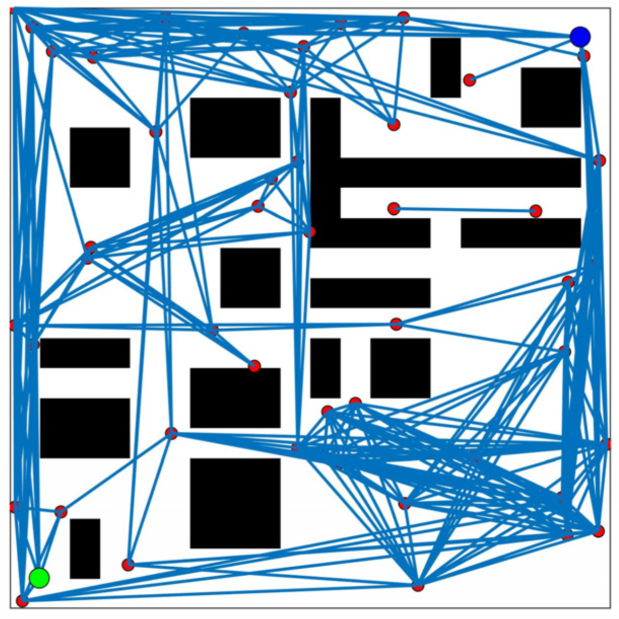
3.1. LCPP for Path Planning of Multiple USVs

The visibility graph method (VG) takes the start point $P_s$, target point $P_t$, and vertices $P_{oi}$ of polygonal obstacles as the vertices, connects these vertices to each other, and preserves the lines that do not cross obstacles as visible edges [21]. In Figure 4, the paths are planned from the start point $P_s$ to the target point $P_t$ using VG in an area with two obstacles. The gray rectangle represents obstacles and the blue line segment represents the planned path.

The key for VG is to determine whether the line between any two vertices passes through an obstacle. It can directly detect whether the line between any two vertices passes through an obstacle or simplify the judgment by using the following methods [21]: (1) the line between adjacent vertices of the same obstacle does not pass through the obstacle, and the line between non-adjacent vertices of the same convex obstacle passes through the obstacle; (2) the determination of whether the line connecting the vertices of different obstacles passes through an obstacle can be transformed into determining whether its vertex line intersects with the edges that make up the obstacle.

LCPP is shown in Algorithm 1, as a low-complexity path-planning algorithm for multiple USVs based on VG.

Algorithm 1.

In order to improve the path safety of USVs and reduce the computational complexity of planning paths and subsequent screening of the shortest path, LCPP adds safety boundaries and reduces the number of planned paths based on VG. The main purpose of LCPP is to construct the safety boundary of obstacles and the path between the starting point, target point, and obstacles. The path of LCPP can be divided into the following three types:

(1)

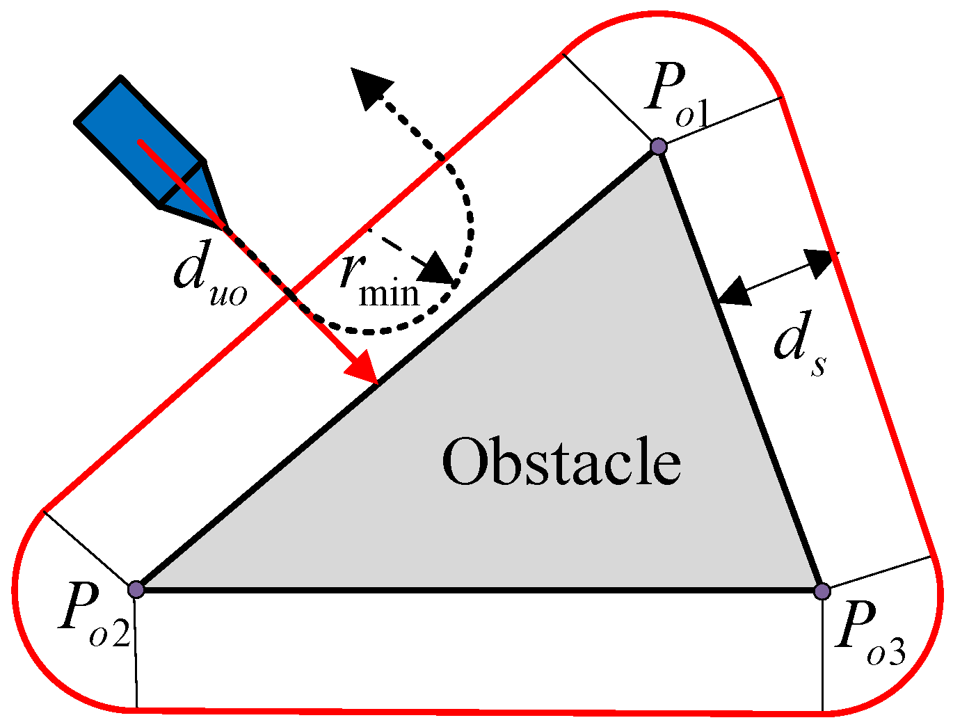
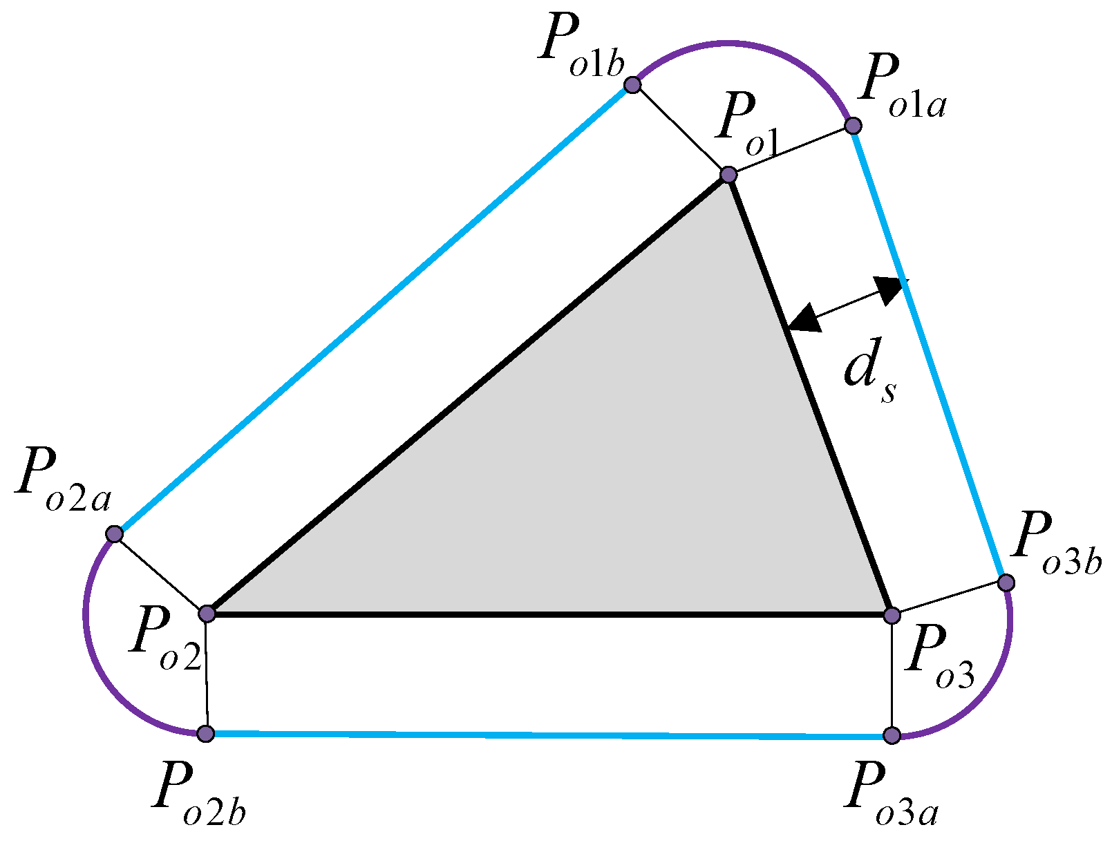
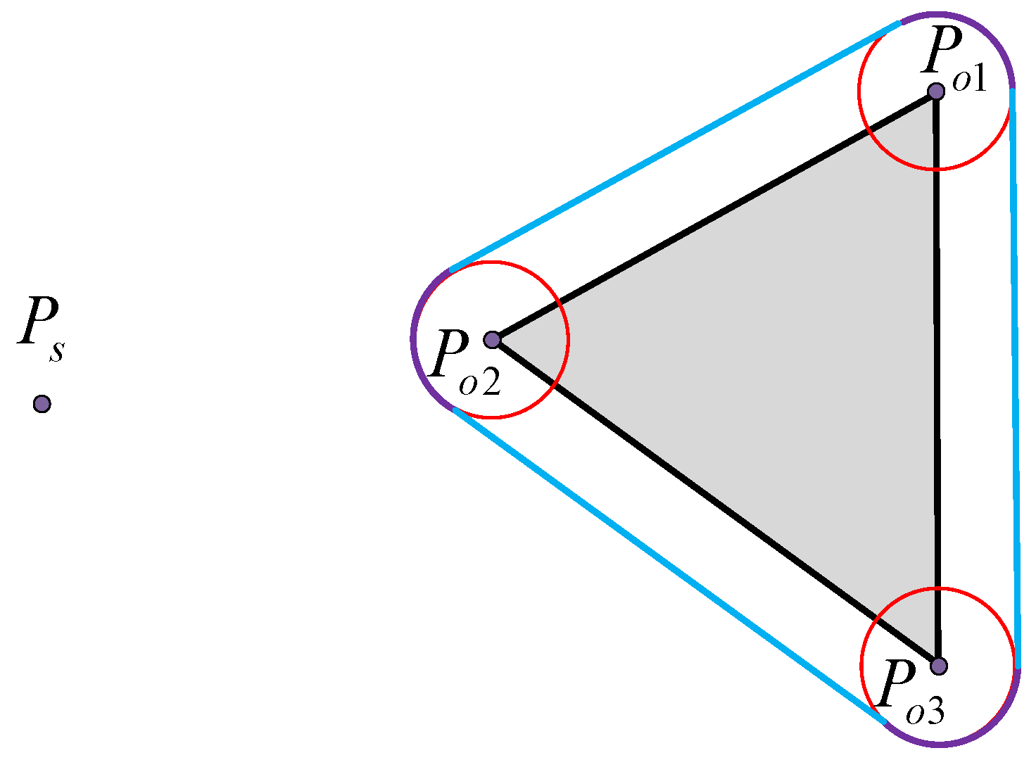
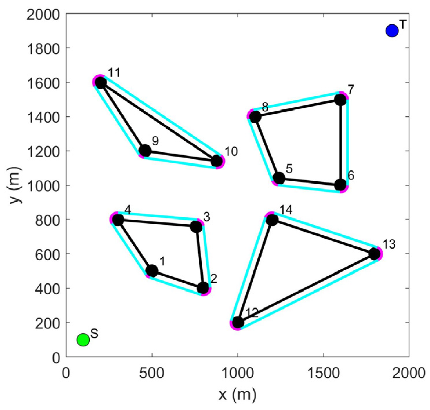
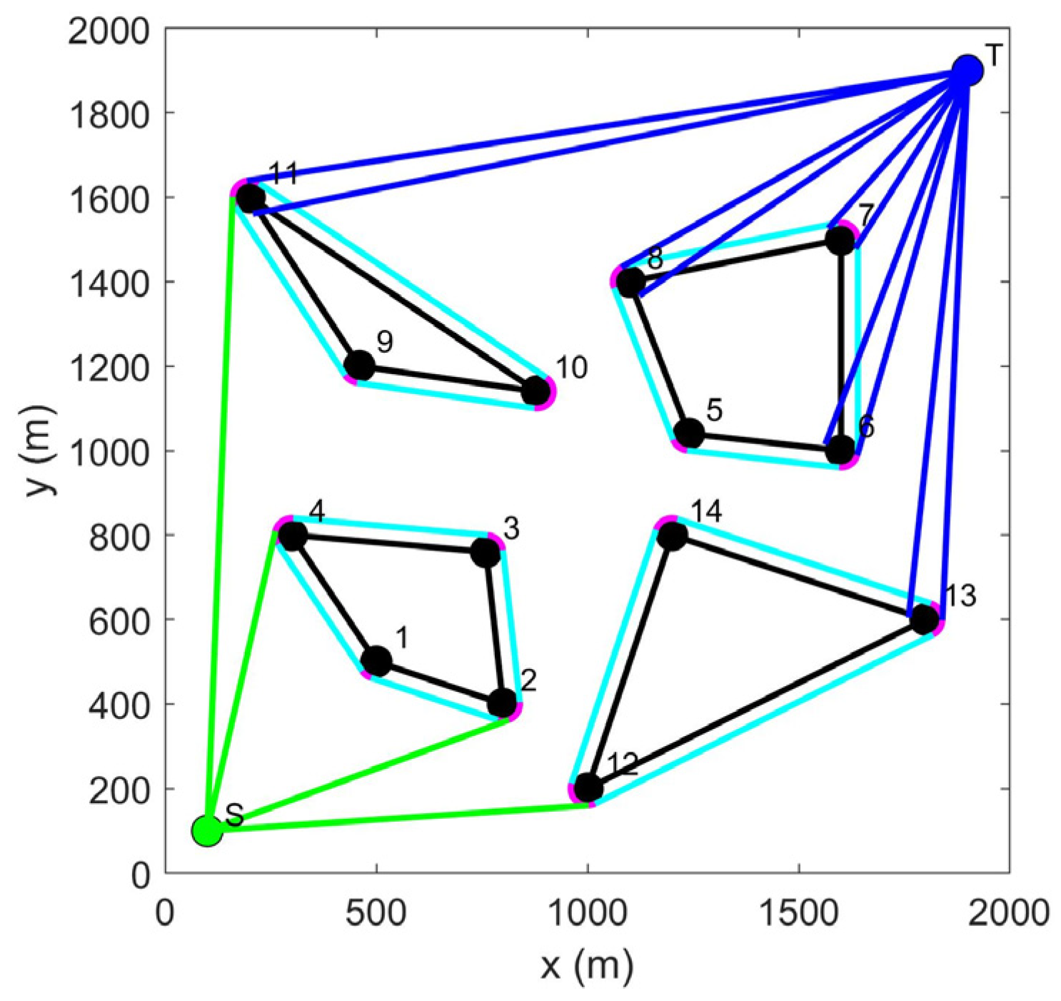
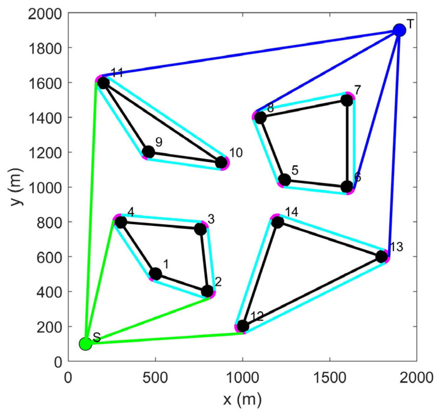
The path along the safety boundary of obstacles. The safety boundary of the obstacle vertex is represented by a circular arc and is tangential to the safety boundary of the connected straight line.

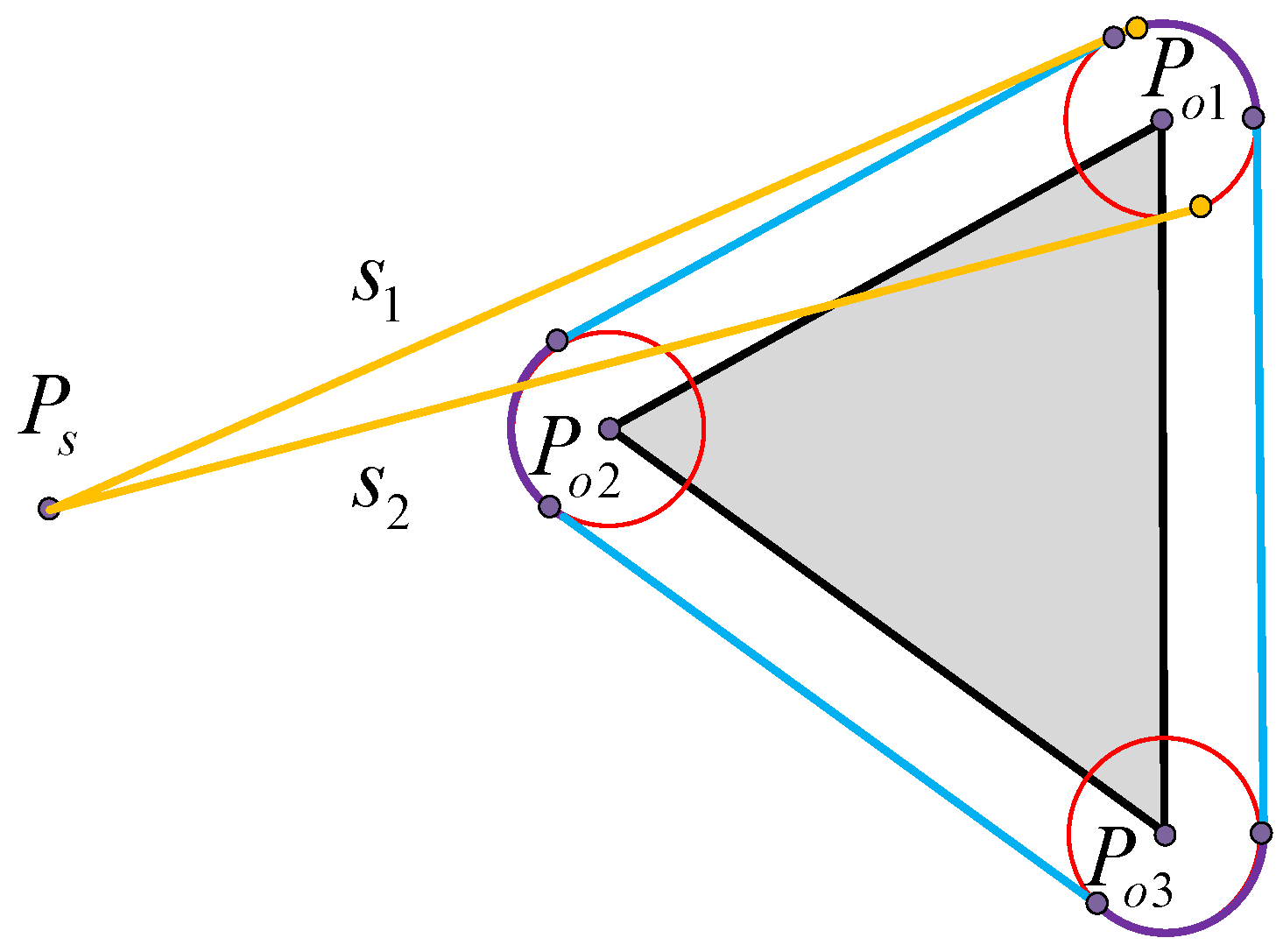
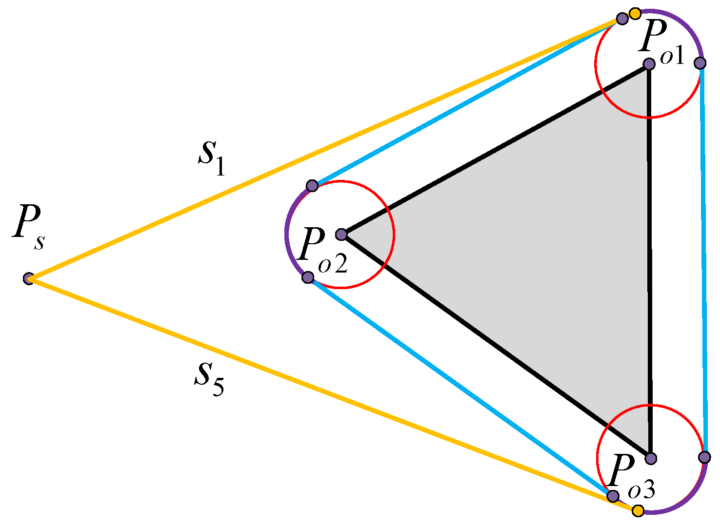
Example 1.

As shown in Figure 5, the arc $P_{o1a}{P}_{o1b}$ is the safe boundary of the vertex $P_{o1}$, and the safe distance is $d_s$. In the figure, the arcs $P_{o1a}{P}_{o1b}$, $P_{o2a}{P}_{o2b}$, and $P_{o3a}{P}_{o3b}$ and lines $P_{o1b}{P}_{o2a}$, $P_{o2b}{P}_{o3a}$, and $P_{o3b}{P}_{o1a}$ are the paths in LCPP.

(2)

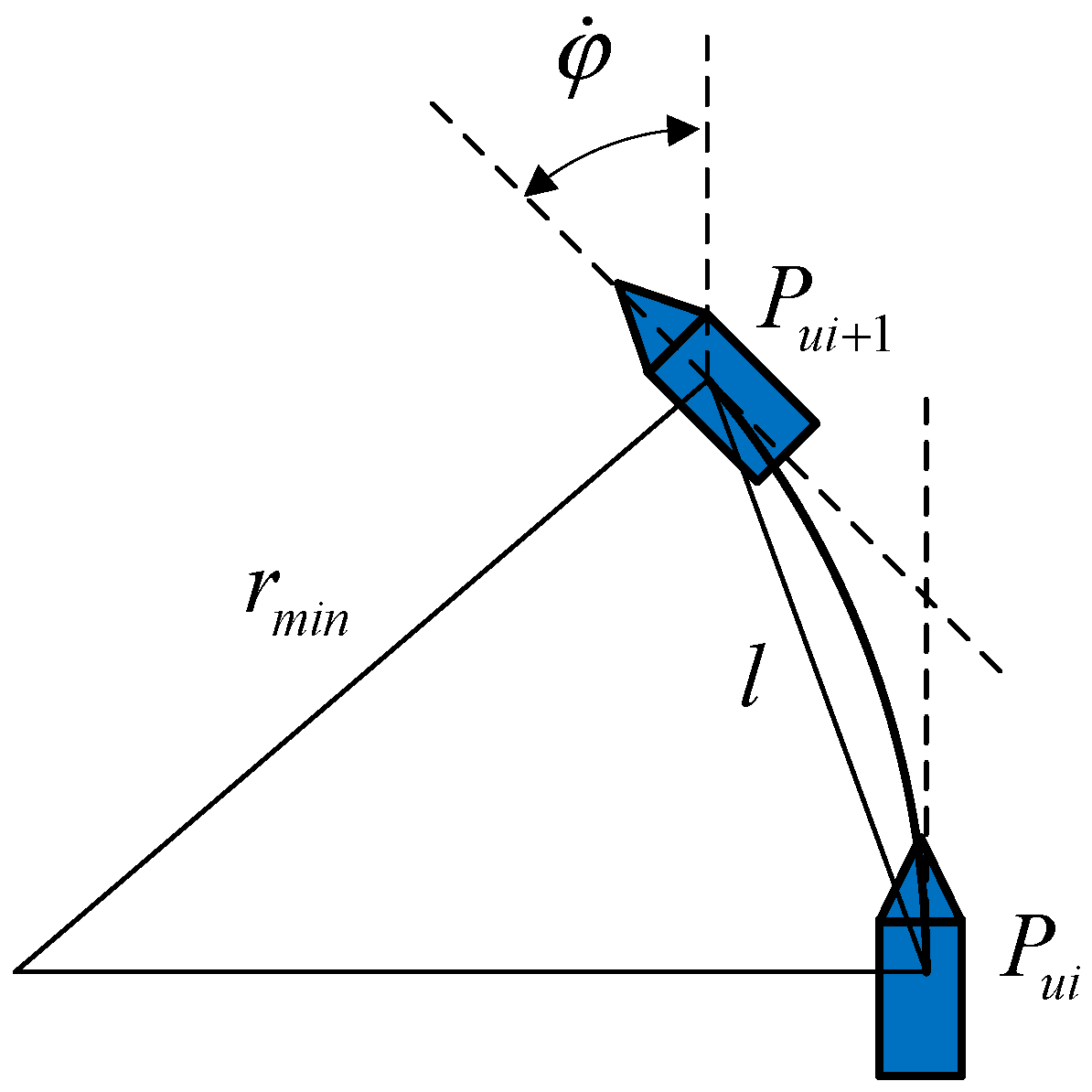
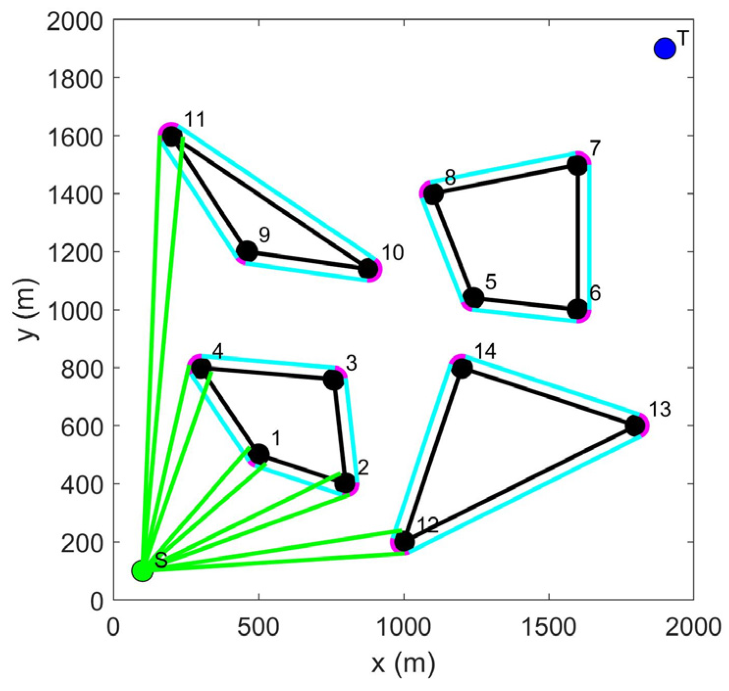
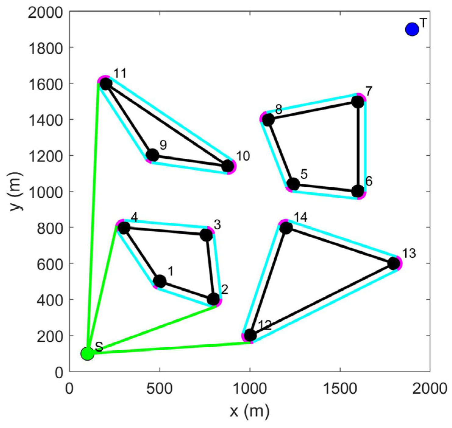
The path from the start point and target point to the vertex of the obstacle. Because the starting and target points are the locations where USVs depart and arrive, the path from the start and target points to the obstacle vertex should be the tangent of the arc from the start and target points to the obstacle vertex. When the tangent point of the tangent falls on the safe arc corresponding to the vertex, the tangent is an optional path. When the USV moves toward the target point, if it needs to update the path, the path from the USV to the obstacle vertex needs to be recalculated because the USV has moved from the start point to a new position. The target point is always stationary, so there is no need to recalculate the path from the target point to the obstacle vertex.

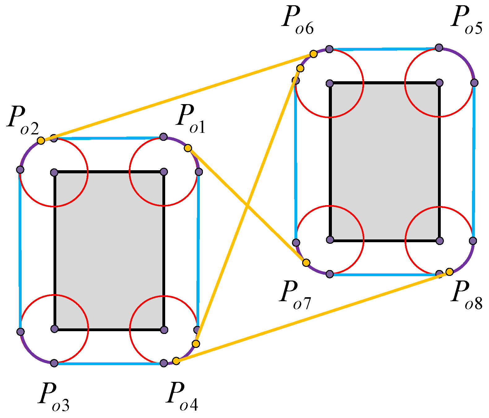
Example 2.

As shown in Figure 6, we take the initial state of the starting point and obstacle safety boundary. We filter the two tangent lines from the start point to the safety circle of $P_{o1}$ in Figure 7, where the tangent point of the route $s_1$ falls on the corresponding safety arc of $P_{o1}$, and $s_1$ is therefore an optional path. If the tangent point of the route $s_2$ does not fall on the safe arc, it is an abandoned path that cannot be chosen. Similarly, as shown in Figure 8, both the route $s_3$ and the route $s_4$ are nonselectable abandoned paths. The final optional path result is shown in Figure 9, where only route $s_1$ and route $s_5$ are optional paths.

(3)

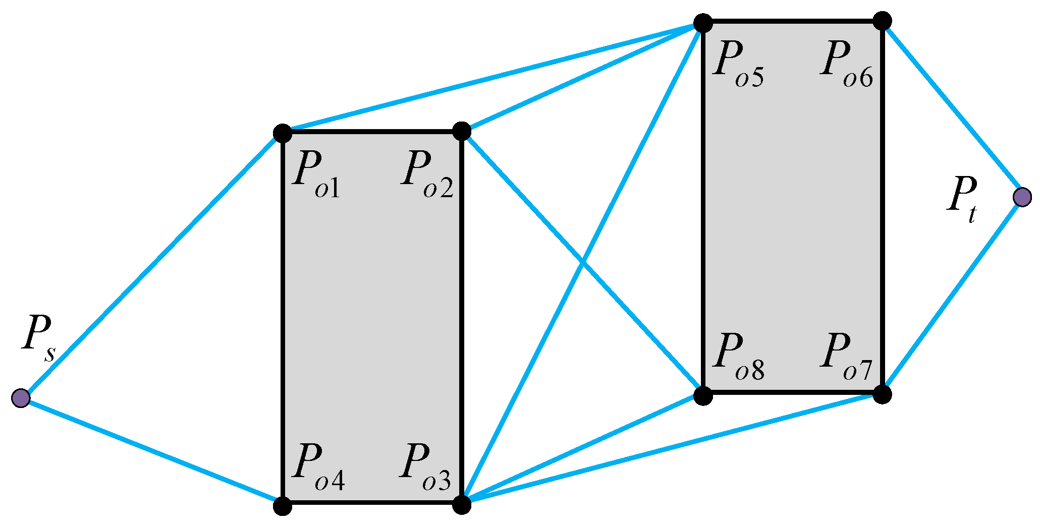
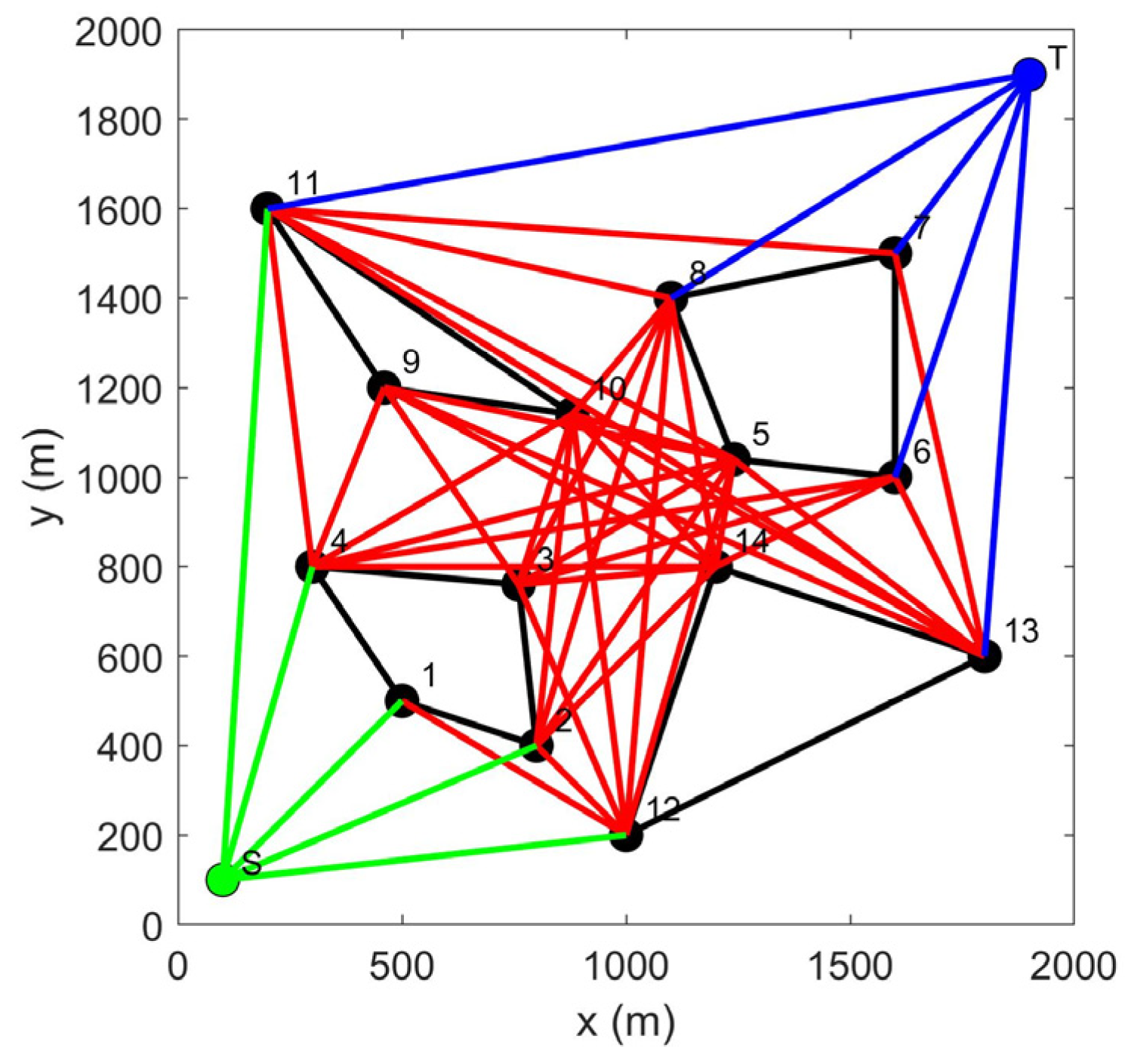
The path between the vertices of obstacles. The path between obstacle vertices is based on VG to select feasible theoretical paths, construct a safe circle for obstacle vertices, construct four tangents between vertex safe circles, and observe the position of the tangents. If both tangent points of the tangent line are on the safe arc, then the path is an optional path and other paths are unsafe and unselected abandoned paths. Judging the path between obstacle vertices in this way not only increases the safety of the path but also eliminates nonselectable paths in advance, reducing the filtering range for subsequent selectable path selections.

Example 3.

As shown in Figure 10, the blue line is the optional path extended by the obstacle edge, the purple arc is the safety arc extended by the obstacle vertex, and the yellow line is the four tangent lines between the corresponding safety circles of the vertex $P_{o4}$ and $P_{o8}$. Only tangents with all tangent points on the safe arc are optional paths, so based on the positions of the eight tangent points corresponding to the four tangents, only route $s_4$ is an optional path. Two obstacles each have four vertices. If the vertices of the same obstacle are also judged, 28 calculations are required, and there is no need to use tangents to judge the vertices themselves. As shown in Figure 11, LCPP has four selectable paths between two obstacle vertices, while VG corresponds to six paths. In comparison, the improved selectable paths are safer and have fewer options, which is beneficial for reducing the filtering range in subsequent path selection.

Remark 1.

In theory, the complexity of LCPP is related to the number of USVs and the number of vertices of obstacles. However, in map-based path planning, the number of vertices of obstacles is usually fixed. Therefore, in environments where only fixed obstacles exist, LCPP for path planning of multiple USVs can be regarded as only related to the number of USVs.

Remark 2.

The path planning for multiple USVs in task planning is to plan the paths of each USV to each target point, which requires planning $n^2$ paths, and the computational complexity is $O\left(n^2\right)$. However, according to the calculation process of LCPP, the path between obstacle vertices only needs to be calculated once, the path from $n$ start points to obstacles needs to be planned $n$ times, and the path from $n$ target points to obstacles needs to be planned $n$ times. Therefore, the planning complexity of LCPP is only $O\left(n\right)$. In the path planning of a large number of USVs, the lower the complexity, the better. Therefore, LCPP is a better low-complexity path-planning algorithm than other algorithms for multiple USVs in task planning.

Example 4.

The initial environment for comparing LCPP and VG is shown in Figure 12. The calculation results of VG are shown in Figure 13, where the green lines represent the path from the start point to the vertex of the obstacle, with five lines. The blue lines represent the path from the target point to the vertex of the obstacle, with five lines. The red straight line is the path from the vertex of the obstacle to the vertex of the obstacle, with 39 lines.

As shown in Figure 14, we construct safety boundaries for the four obstacles on the map. The light blue straight line is the straight part of the obstacle safety boundary, and the purple arc is the curved part of the safety boundary. As shown in Figure 15 and Figure 16, there are 10 optional paths starting from the starting point, and 4 remaining paths. As shown in Figure 17 and Figure 18, there are 10 optional paths starting from the target point, and 4 remaining paths. By judging the paths between all obstacle vertices, 20 paths from obstacle vertices to obstacle vertices can be obtained, represented by the red lines shown in Figure 19.

Since the Dijkstra algorithm calculates the weights (path lengths) from the start point to all nodes in the graph, it can calculate the shortest path from one start point to $n$ target points at a time. The path planning for multiple USVs in task planning is to plan the paths of $n$ USVs to $n$ target points, usually requiring planning $n^2$ paths. However, the Dijkstra algorithm only needs to be calculated $n$ times, and the computational complexity is $O\left(n\right)$, as shown in Figure 20 and Figure 21.

There are 16 paths from each starting point to each target point. The paths from the same starting point to all target points are calculated each time using the Dijkstra algorithm, as shown in Figure 22, Figure 23, Figure 24 and Figure 25.

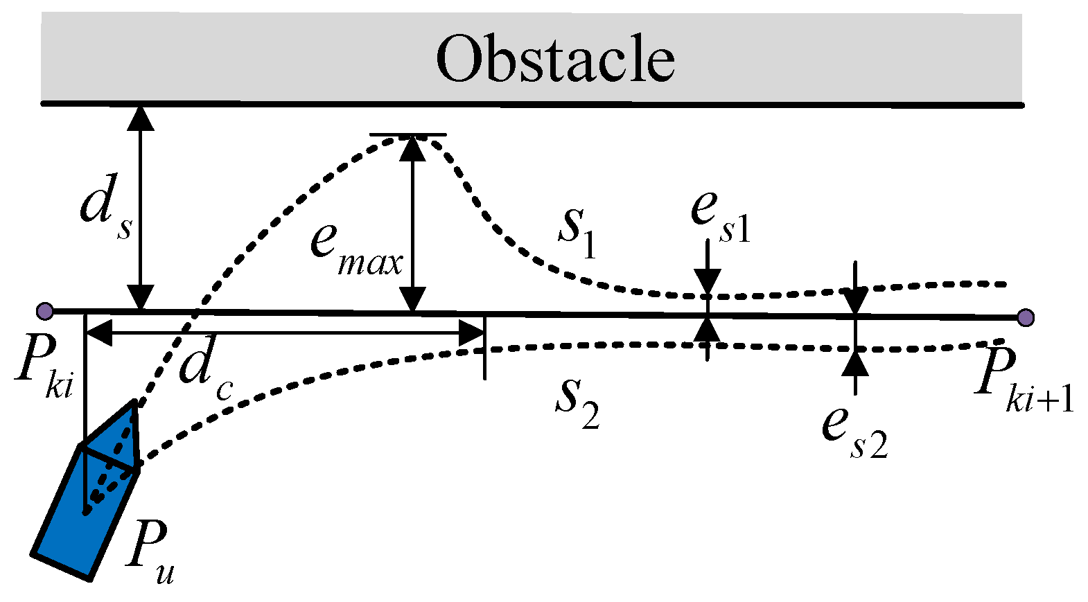
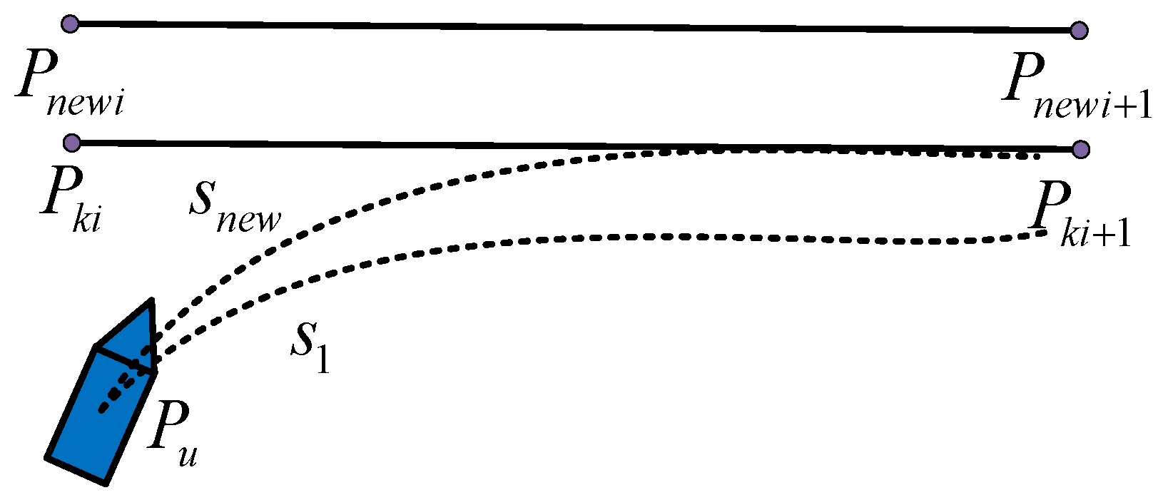
3.2. ALOS with the Optimized Parameter

The LOS guidance law [22] is based on the lookahead distance and projection, as shown in Figure 26.

In the process of guidance, we only need to control the heading $\phi$ of the USV to the desired heading ${\phi }_{los}$ of LOS to ensure the cross-track error $y_e$ is equal to 0, as shown in (5) and (6). ${\alpha }_{ki}$ is the angle of the path relative to the true north. $\beta$ is the sideslip angle. ${\alpha }_{los}$ is the desired angle of LOS to minimize the cross-track error.

$$\phi \to {\phi }_{los}={\alpha }_{ki}-\beta +{\alpha }_{los}$$

(5)

$$\underset{t\to +\infty }{\mathit{lim}}{y}_e=0$$

(6)

The desired path consists of a series of path points $P_{ki}=\left(x_{ki},y_{ki}\right)$. $P_{ki}$ and $P_{ki+1}$ form a straight path, ${\alpha }_{ki}$ can be calculated as shown in (7). In the curve guidance, ${\alpha }_{ki}\left(\theta \right)$ can be calculated, as shown in (8), for any point $P_{ki}\left(\theta \right)=\left(x_{ki}\left(\theta \right),y_{ki}\left(\theta \right)\right)$ on the desired path [23].

$${\alpha }_{ki}=atan2\left(y_{ki+1}-y_{ki},x_{ki+1}-x_{ki}\right)$$

(7)

$${\alpha }_{ki}\left(\theta \right)=atan2\left(y_{ki+1}\left(\theta \right)-y_{ki}\left(\theta \right),x_{ki+1}\left(\theta \right)-x_{ki}\left(\theta \right)\right)$$

(8)

The desired point of LOS is $P_{los}=\left(x_{los},y_{los}\right)$. According to the geometric relationship, the lookahead distance $\mathsf{\Delta }$, cross-track error $y_e$, and ${\alpha }_{los}$ can be calculated, as shown in (9) and (10).

$$y_e=-cos{\alpha }_{ki}\left(x_u-x_{ki}\right)+sin{\alpha }_{ki}\left(y_u-y_{ki}\right)$$

(9)

$${\alpha }_{los}=atan2\left(y_e,\mathsf{\Delta }\right)$$

(10)

In the ALOS with the lookahead distance [24,25], the steady-state error $e_s$ is zero. $k$ in (11) can be adjusted to reduce the maximum error $e_{max}$ and convergence time $t_c$. ${\mathsf{\Delta }}_{max}$ and ${\mathsf{\Delta }}_{min}$ are the maximum and minimum lookahead distances and $e$ is the natural constant. The maximum error $e_{max}$ corresponds to the safety of the USV, and the convergence time $t_c$ corresponds to controllability. Therefore, it is necessary to find a suitable $k$ based on the specific weight function $f_w$ and the optimization algorithm to reduce the maximum error $e_{max}$ and convergence time $t_c$.

$$\mathsf{\Delta }\left(y_e\right)=\left({\mathsf{\Delta }}_{max}-{\mathsf{\Delta }}_{min}\right)e^{-k{y_e}^2}+{\mathsf{\Delta }}_{min}$$

(11)

The important parameters of the USV trajectory after guidance include the maximum error $e_{max}$, the steady state error $e_s$, and the convergence time $t_c$, as shown in Figure 27 and (12). When the USV trajectory is between the safe boundary and the obstacle, $y_e$ is negative, indicating more danger. Error outside the safe boundary is relatively safe. In the figure, the trajectory $s_1$ is more dangerous than the trajectory $s_2$.

$$\begin{gathered} t_c=\mathit{min}\text{{}t|\left|y_e\left(t+1\right)-y_e\left(t\right)\right|<a_s\} \\ {e}_s=y_e\left(t_c\right) \\ {e}_{max}=\mathit{min}\left(y_e\left(t\right)\right) \end{gathered}$$

(12)

Although ALOS can eliminate steady-state errors in straight paths, it may not be possible to completely eliminate steady-state errors in curved paths due to the rapid switching of desired path points. By changing the desired path, the steady-state error $e_s$ can be reduced, and the actual trajectory can be stabilized at the desired path, as shown in Figure 28. The desired path $P_{ki}{P}_{ki+1}$ is changed to $P_{newi}{P}_{newi+1}$, so that the trajectory $s_{new}$ is exactly stable on the originally expected path $P_{ki}{P}_{ki+1}$. Therefore, the steady-state error $e_s$ can be reduced by changing the desired path when designing the desired path.

The algorithm for calculating the evaluation parameter $y_w\left(k\right)$ is shown in Algorithm 2.

Algorithm 2. Calculate evaluation parameter $y_w\left(k\right)$
Input: $k$, USV motion model $f_m$, USV control algorithm $f_c$, LOS algorithm $f_{los}$, weighting function $f_w$, end time of LOS $t_{end}$, initial position $P_{u0}$, initial speed $v_0$, and initial heading ${\phi }_0$ of USV, desired path $P_{ki}{P}_{ki+1}$, ${\mathsf{\Delta }}_{max}$, ${\mathsf{\Delta }}_{min}$
Output: evaluation parameter $y_w\left(k\right)$
1:	$i=0$;
2:	While $i<t_{end}$
3:	$y_e\leftarrow \left(P_{ui},P_{ki}{P}_{ki+1}\right)$; // track error
4:	${\phi }_{di}=f_{los}\left({\mathsf{\Delta }}_{max},{\mathsf{\Delta }}_{min},y_e,k\right)$; // desired heading
5:	${\delta }_i=f_c\left({\phi }_{di}\right)$; // desired rudder angle
6:	$\left(P_{ui+1},v_{i+1},{\phi }_{i+1}\right)=f_m\left(P_{ui},v_i,{\phi }_i,{\delta }_i\right)$; // USV travels
7:	$i=i+1$;
8:	End
9:	$(t_c,e_s,e_{max})\leftarrow \left\{y_e\right\}\leftarrow (\left\{P_u\right\},\left\{P_k\right\}$);
10:	$y_w\left(k\right)=f_w(t_c,e_s,e_{max})$;

In (11), $k$ in ALOS is a single variable, so a simple and flexible simulated annealing algorithm is suitable for determining $k$ of the formula, as shown in Algorithm 3.

Algorithm 3. Parameter selection of LOS using Simulated Annealing
Input: Initial temperature $T_0$, final temperature $T_f$, attenuation coefficient $\alpha$, initial solution $k_0$, length of Markov chain $l$, random function $f_r$, $y_w\left(k\right)$
Output: Best solution $k_{best}$
1:	$i=0$; $k_{best}=k_0$; $t_k=T_0$; $t=T_0$;
2:	While $t>T_f$ && $i<l$
3:	$k_{i+1}=f_r\left(k_i\right)$;
4:	If $y_w\left(k_{i+1}\right)<y_w\left(k_{best}\right)$
5:	$k_{best}=k_{i+1}$;
6:	Else if $\exp \left(-{\displaystyle \frac{\left(y_w\left(k_{i+1}\right)-y_w\left(k_{best}\right)\right)}{t_k}}\right)\ge \mathrm{rand}\left[0,1\right]$
7:	$k_{best}=k_{i+1}$;
8:	End
9:	$t=\alpha t;$
10:	$i=i+1$;
11:	End

4. Simulation

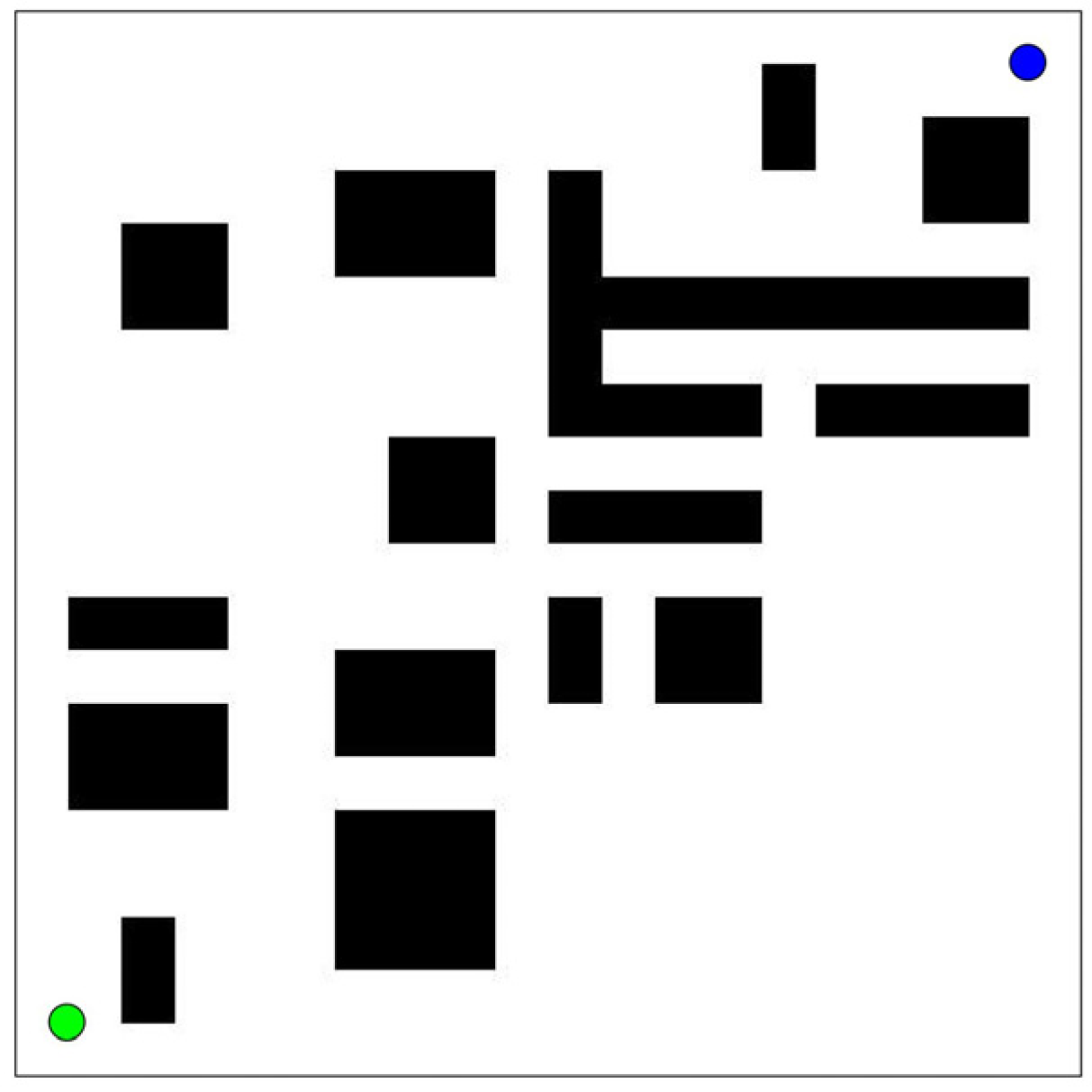
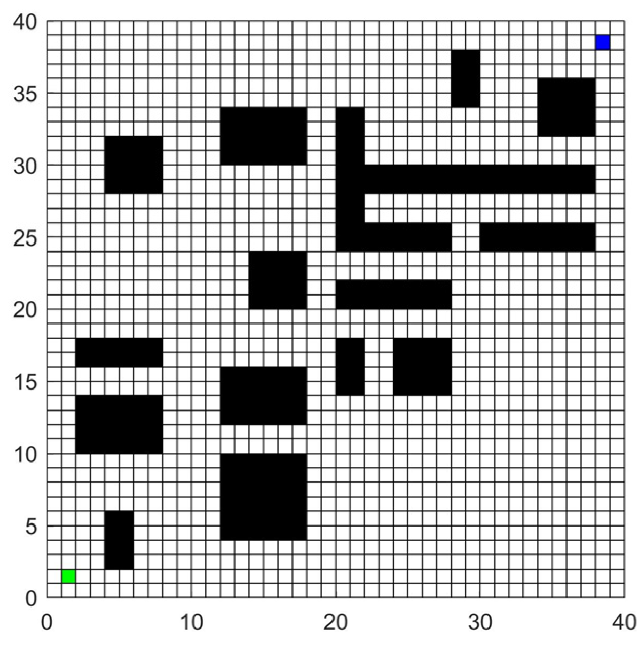
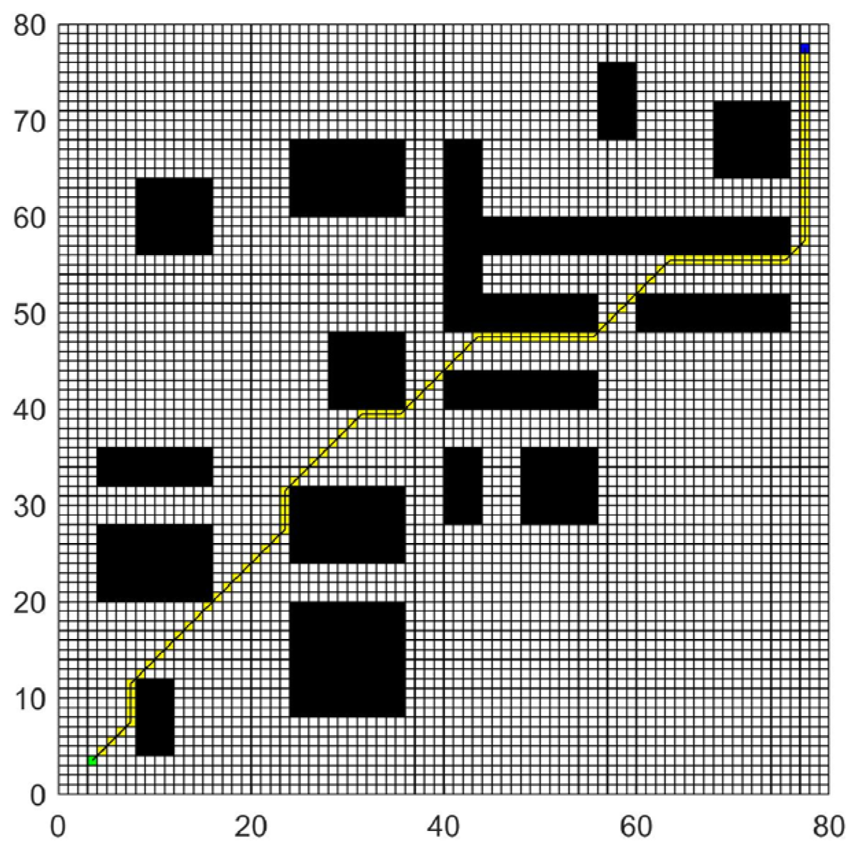
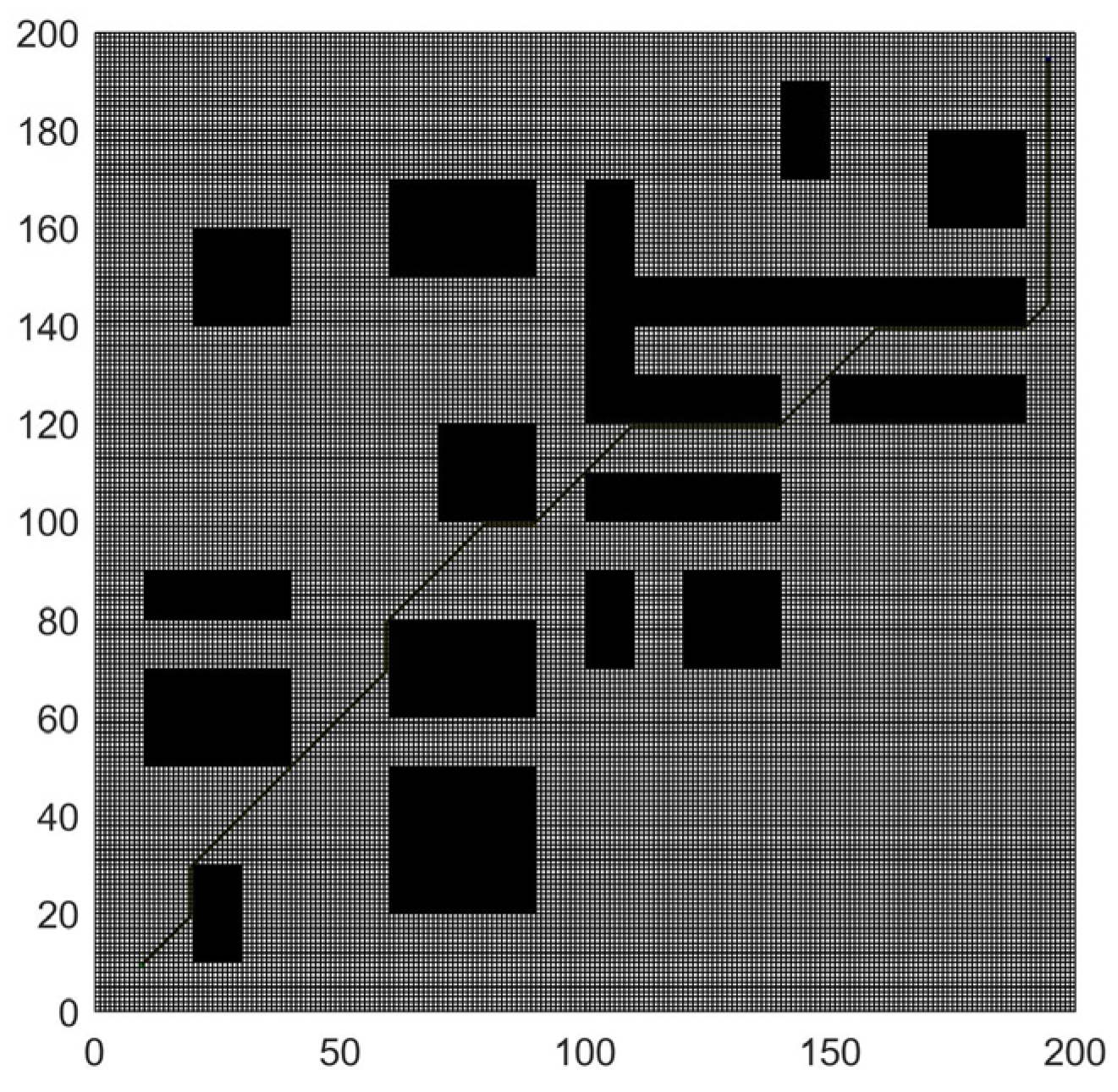
4.1. LCPP for Path Planning of Multiple USVs

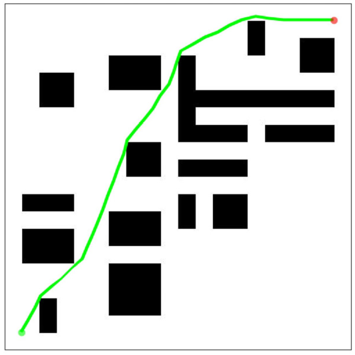
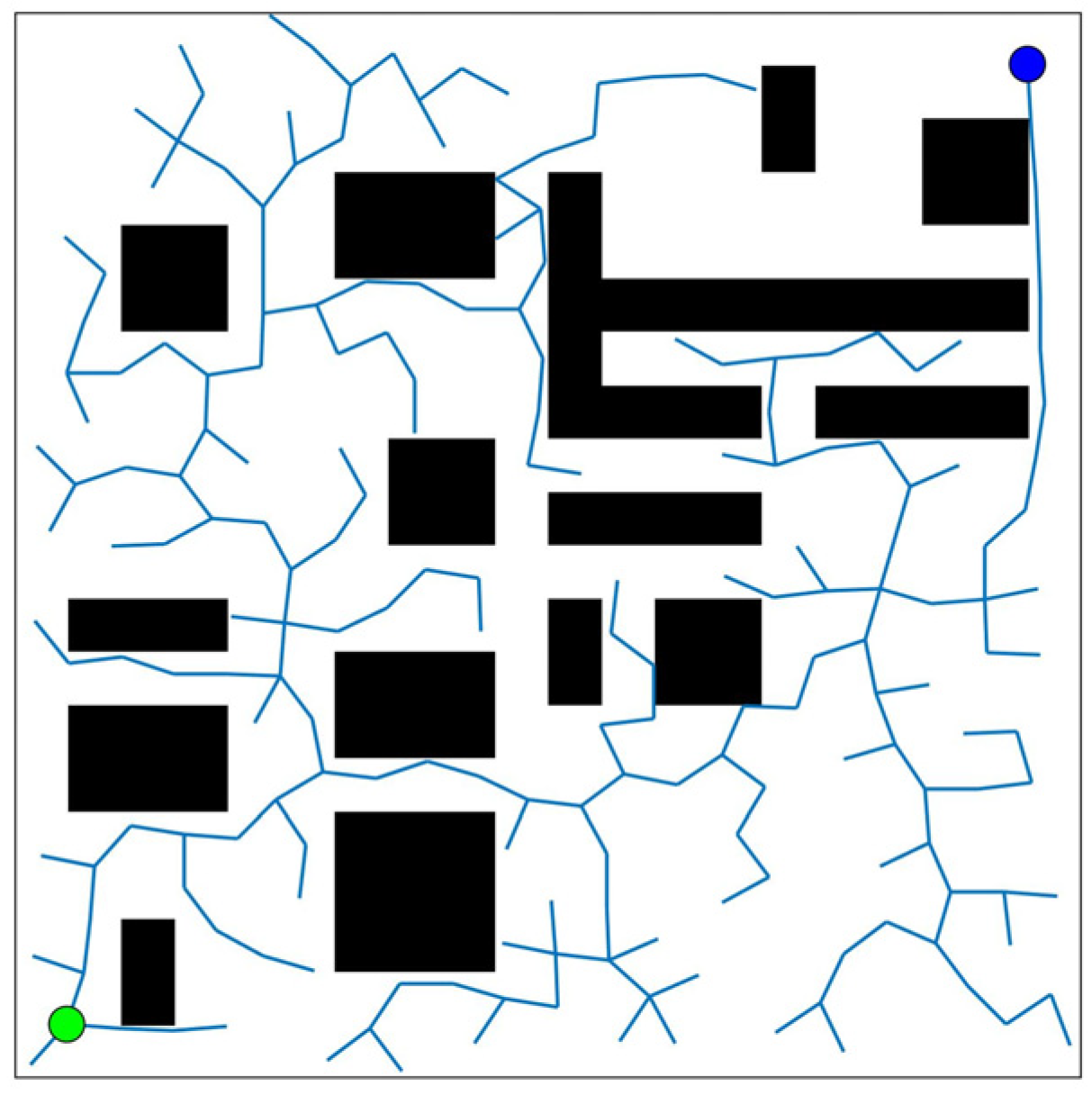
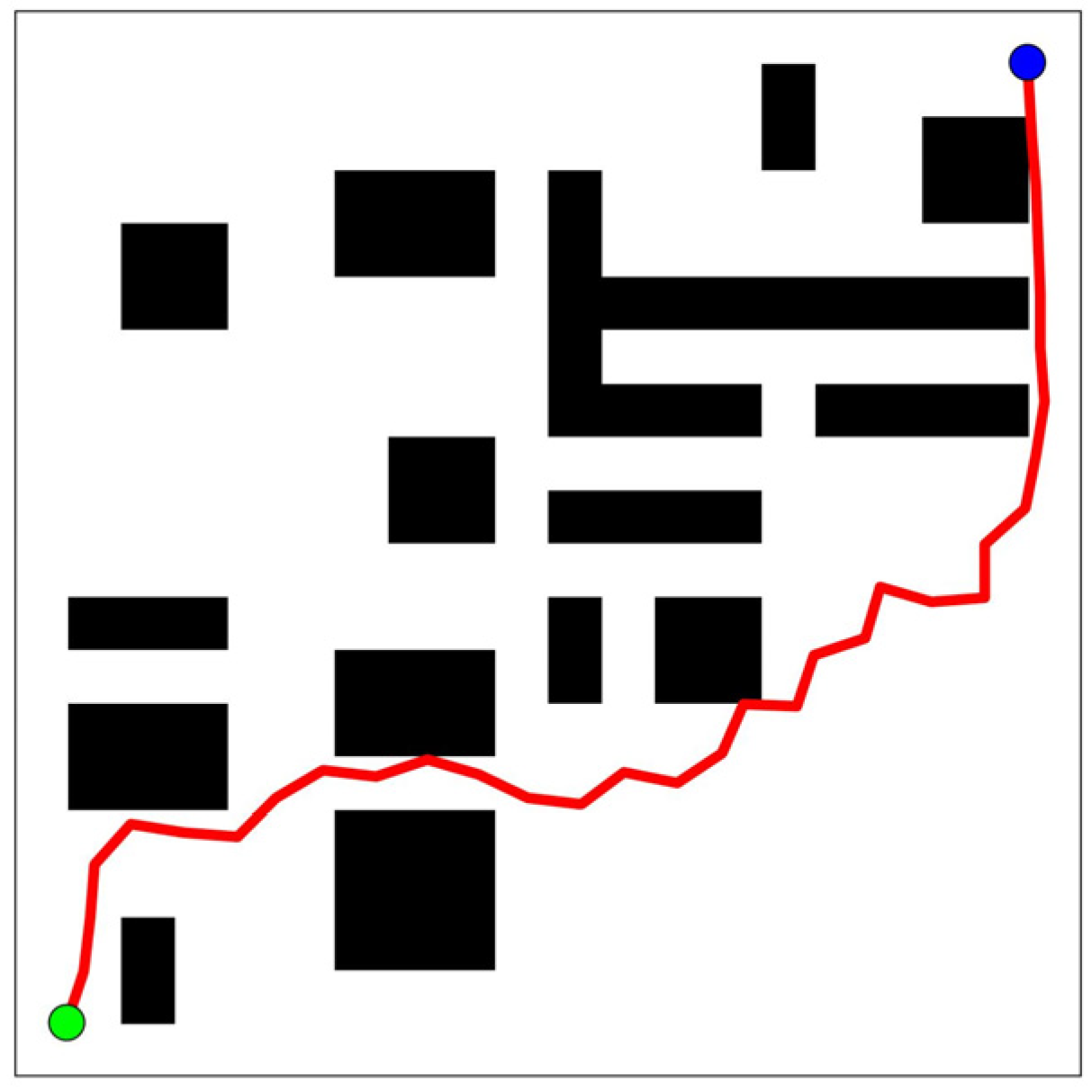
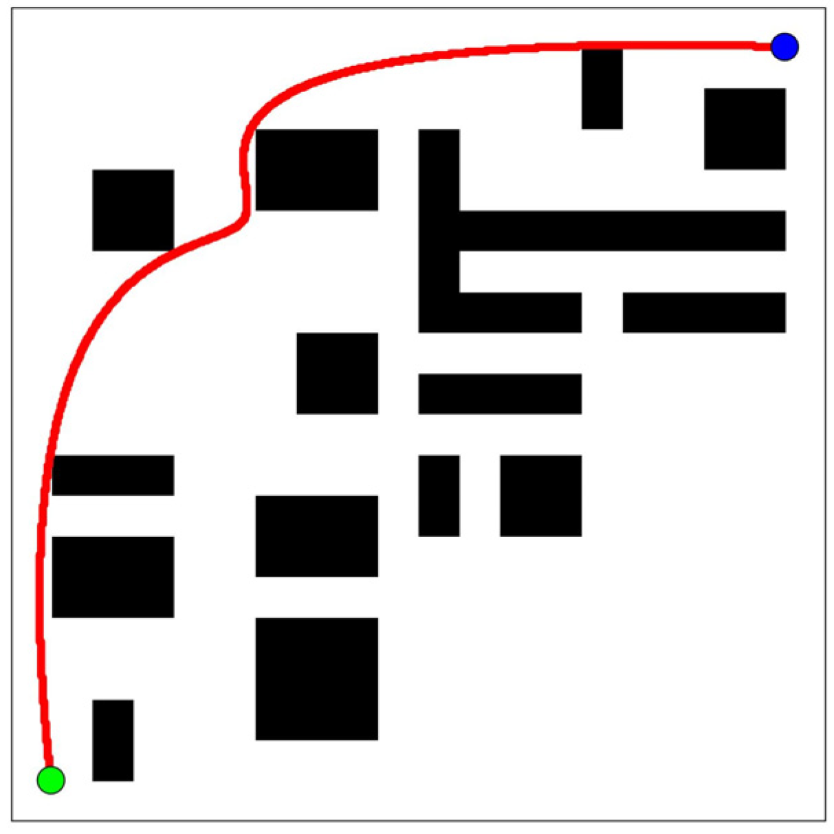
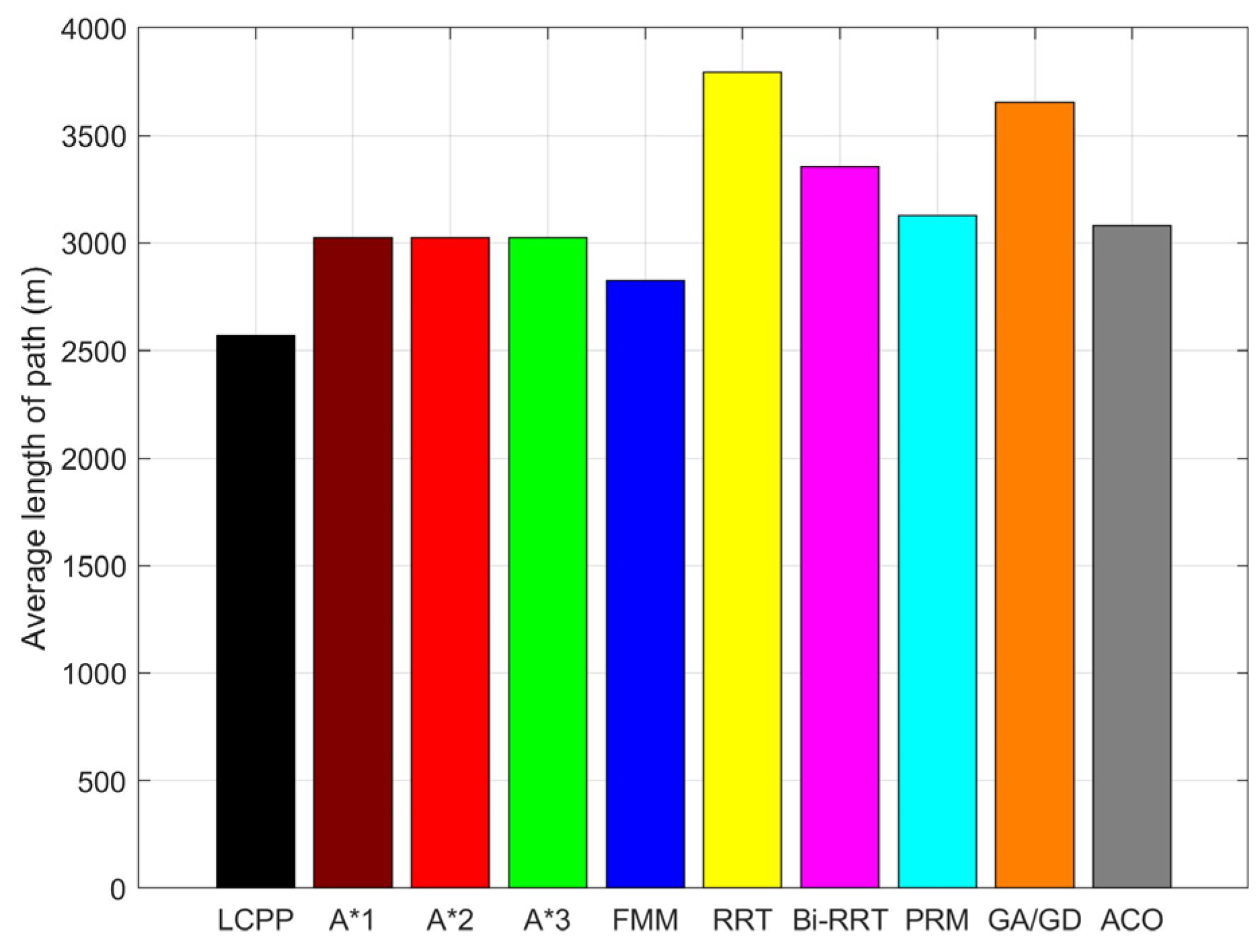
LCPP proposed in this paper is compared with the A * algorithm [26], the Fast Marching Method (FMM) [7,9], the Rapidly Exploring Random Tree algorithm (RRT) [27], the Bidirectional Rapidly Exploring Random Tree algorithm (Bi RRT) [28], the Probabilistic Roadmap algorithm (PRM) [29], the Gradient Descent Genetic Algorithm (GA/GD) [30], and Ant Colony Optimization (ACO) [31]. The algorithms used for comparison in the simulation are shown in

Table 3. Comparison algorithms.

Algorithm	Note
LCPP	Based on VG and using Dijkstra algorithm.
A*1	The grid is 50 m × 50 m
A*2	The grid is 25 m × 25 m.
A*3	The grid is 10 m × 10 m.
FMM	Based on potential field. The minimum potential field unit is 10 m × 10 m, and step length is 80 m.
RRT	Initial step length is 100 m. The minimum step length is 80 m.
Bi-RRT	Step length is 80 m.
PRM	The number of key nodes is 20.
GA/GD	Population size 100, iteration times 1000.
ACO	Population size 100, iteration times 1000.

.

The path planning for multiple USVs in task planning is composed of path planning for the single USV, so the calculation time of the single USV is first analyzed, and then the calculation time and path length of multiple USVs are compared.

(1)

Calculation time and path length of path planning for the single USV

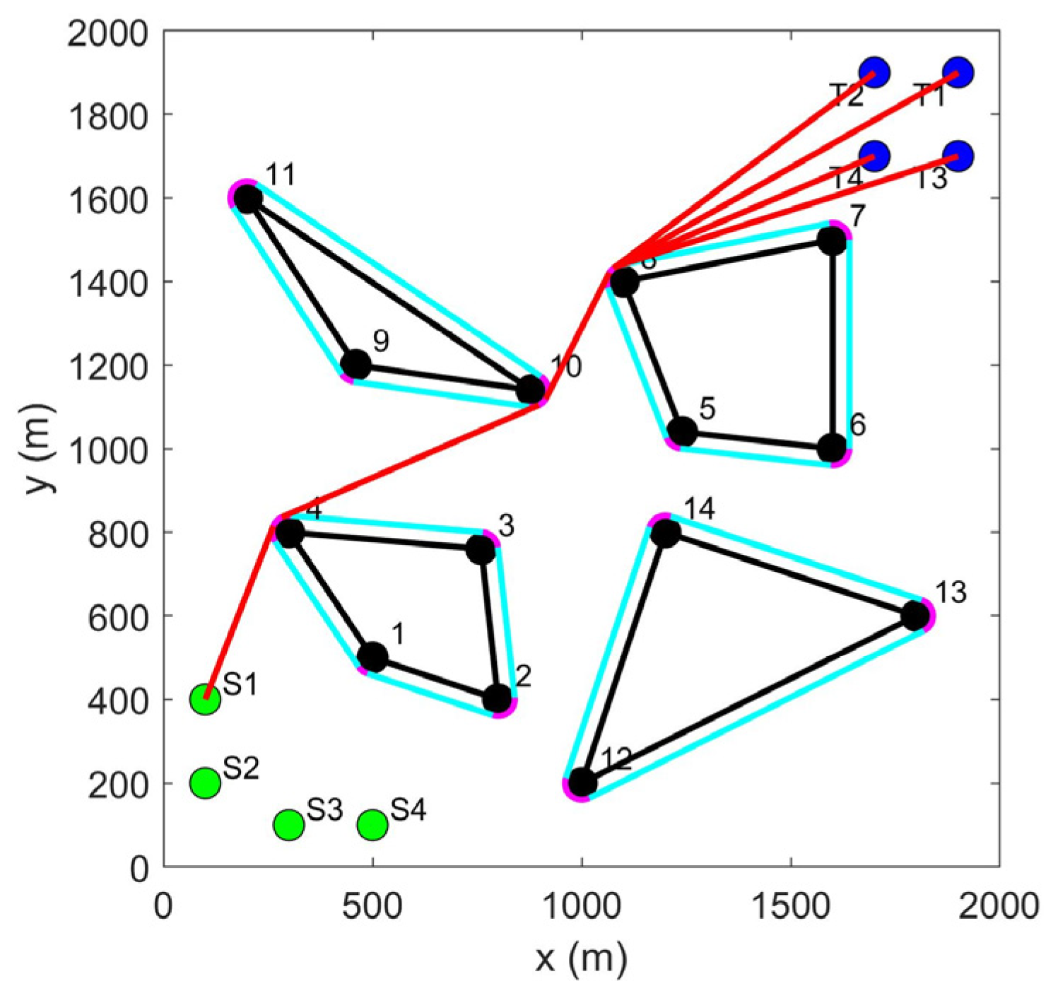
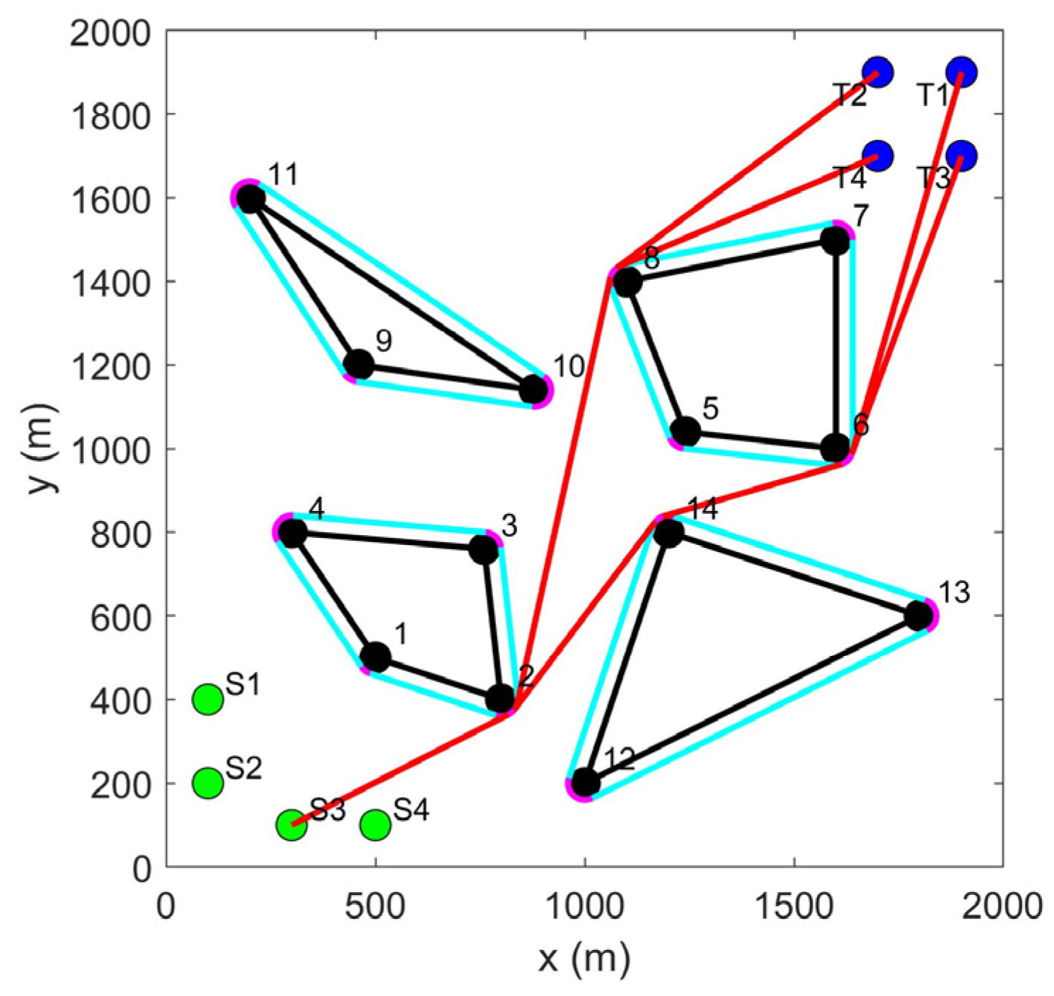
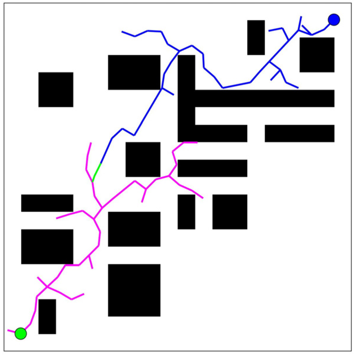
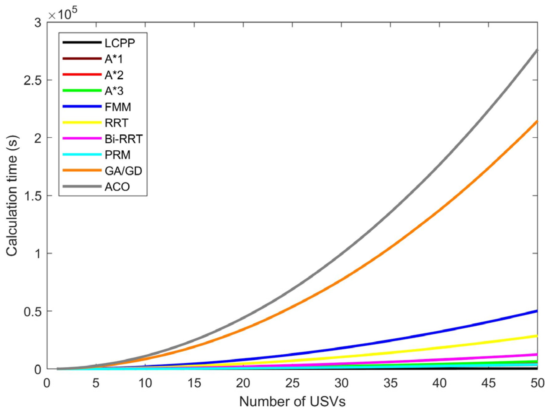
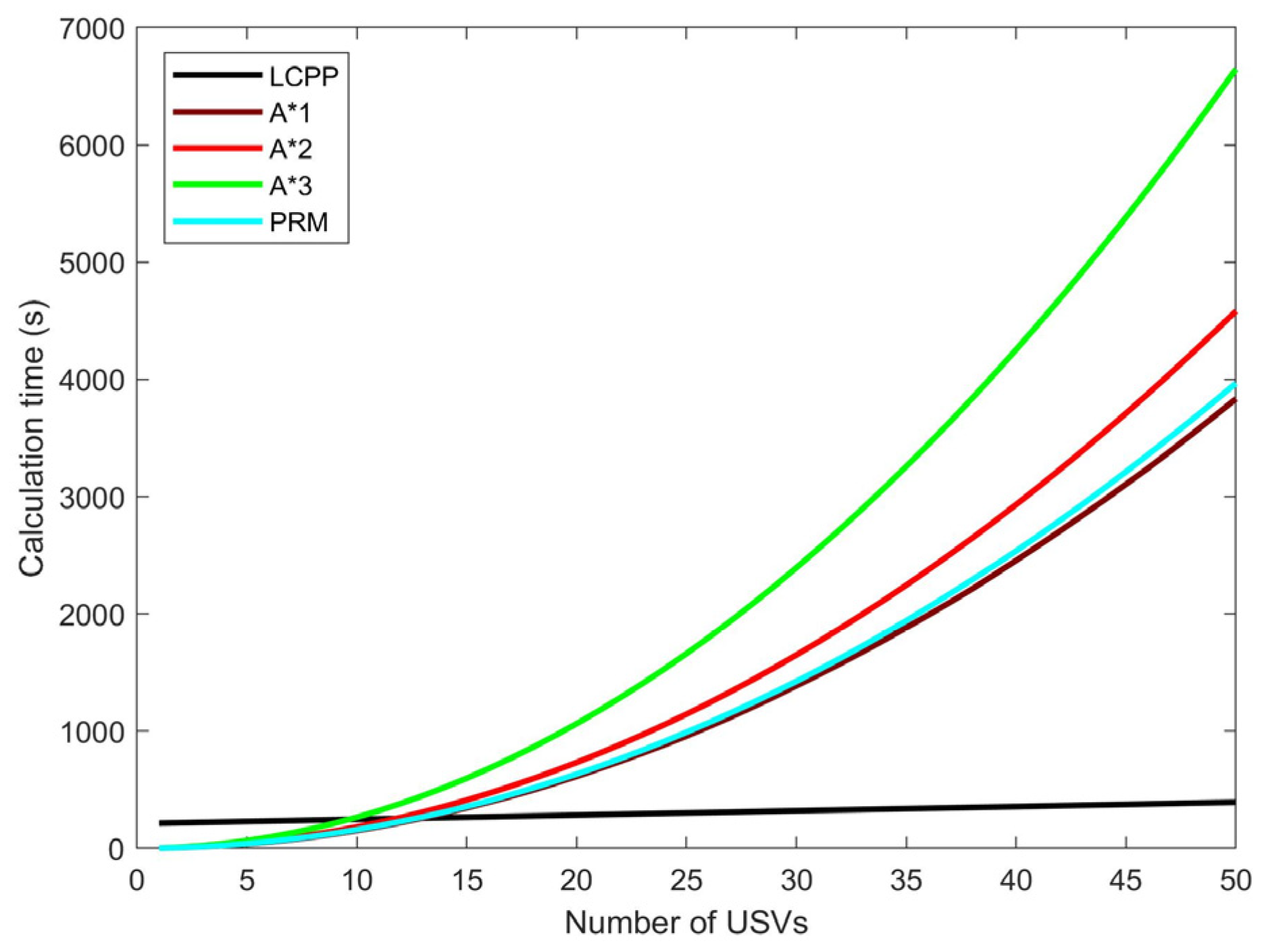
Figure 29 and Figure 30 show the initial maps and the path using LCPP. In Figure 31, Figure 32, Figure 33 and Figure 34, paths are planned using A*1, A*2, and A*3. Figure 35 and Figure 36 show the potential field maps constructed by FMM from the start point to the target point and the paths planned based on potential field gradient descent. Figure 37, Figure 38, Figure 39, Figure 40, Figure 41 and Figure 42 show the random exploration process and planned paths using RRT, Bi RRT, and PRM in the map. Figure 43 and Figure 44 show the paths planned using GA/GD and ACO. The calculation time of these algorithms is shown in

Table 4. Calculation time and path length.

Algorithm	The First Calculation		The Second Calculation		The Third Calculation
	Calculation Time (s)	Path Length (m)	Calculation Time (s)	Path Length (m)	Calculation Time (s)	Path Length (m)
LCPP	215.169	2568.2	The same start point: 0.269 Different start points: 3.960	2568.2	The same start point: 0.721 Different start points: 3.541	2568.2
A*1	1.720	3026.3	1.494	3026.3	1.392	3026.3
A*2	1.847	3026.3	1.826	3026.3	1.827	3026.3
A*3	2.686	3026.3	2.652	3026.3	2.641	3026.3
FMM	19.981	2826.0	19.362	2826.0	21.035	2826.0
RRT	12.570	4111.0	12.060	3831.9	9.799	3447.6
Bi-RRT	6.137	3267.2	4.588	3431.0	4.366	3366.3
PRM	1.513	3084.2	1.533	3032.2	1.716	3273.8
GA/GD	74.840	3548.0	91.038	3744.0	91.408	3664.0
ACO	113.545	3090.1	101.123	3033.6	105.098	3123.3

.

In the figure and table, the LCPP proposed in this paper has a shorter path length compared to other algorithms, and constructing reusable paths between obstacles results in a longer initial calculation time (static obstacles mean the path between obstacles is calculated only once). However, as the number of USVs increases, the calculation time for the same start point increases less, indicating that LCPP is suitable for scenarios with a large number of USVs.

In other path-planning algorithms, the A * algorithm has lower calculation time and path distance values. The FMM plans a shorter path and constructs a potential field map covering the entire map, which takes a longer calculation time. The RRT has a longer calculation time and path length than the Bi-RRT and PRM. GA/GD and ACO have relatively longer calculation times and path lengths according to the population size and iteration times.

(2)

Calculation time and path length of path planning for multiple USVs.

The calculation time of 10 algorithms for path planning from 1 USV (1 path) to 50 USVs (2500 paths) is shown in Figure 45. Among them, the calculation times of FMM, RRT, Bi RRT, GA/GD, and ACO are too long. Therefore, the calculation time of LCPP, A*1, A*2, A*3, and PRM, which are less time-consuming, is further enlarged and compared, as shown in Figure 46.

In the figure, the calculation time of LCPP increases linearly, and the path-planning complexity is only $O\left(n\right)$. The computation time of other algorithms increases exponentially, and their path planning complexity is $O\left(n^2\right)$. Although LCPP initially takes some time to construct the path between obstacles (static obstacles mean the path between obstacles is calculated only once), as the number of USVs increases (such as in Figure 46, where the number of USVs is greater than 14), the calculation time of LCPP will eventually be less than other algorithms.

The average lengths of the paths planned by 10 algorithms are shown in Figure 47. LCPP has the shortest path length.

4.2. ALOS with the Optimized Parameter

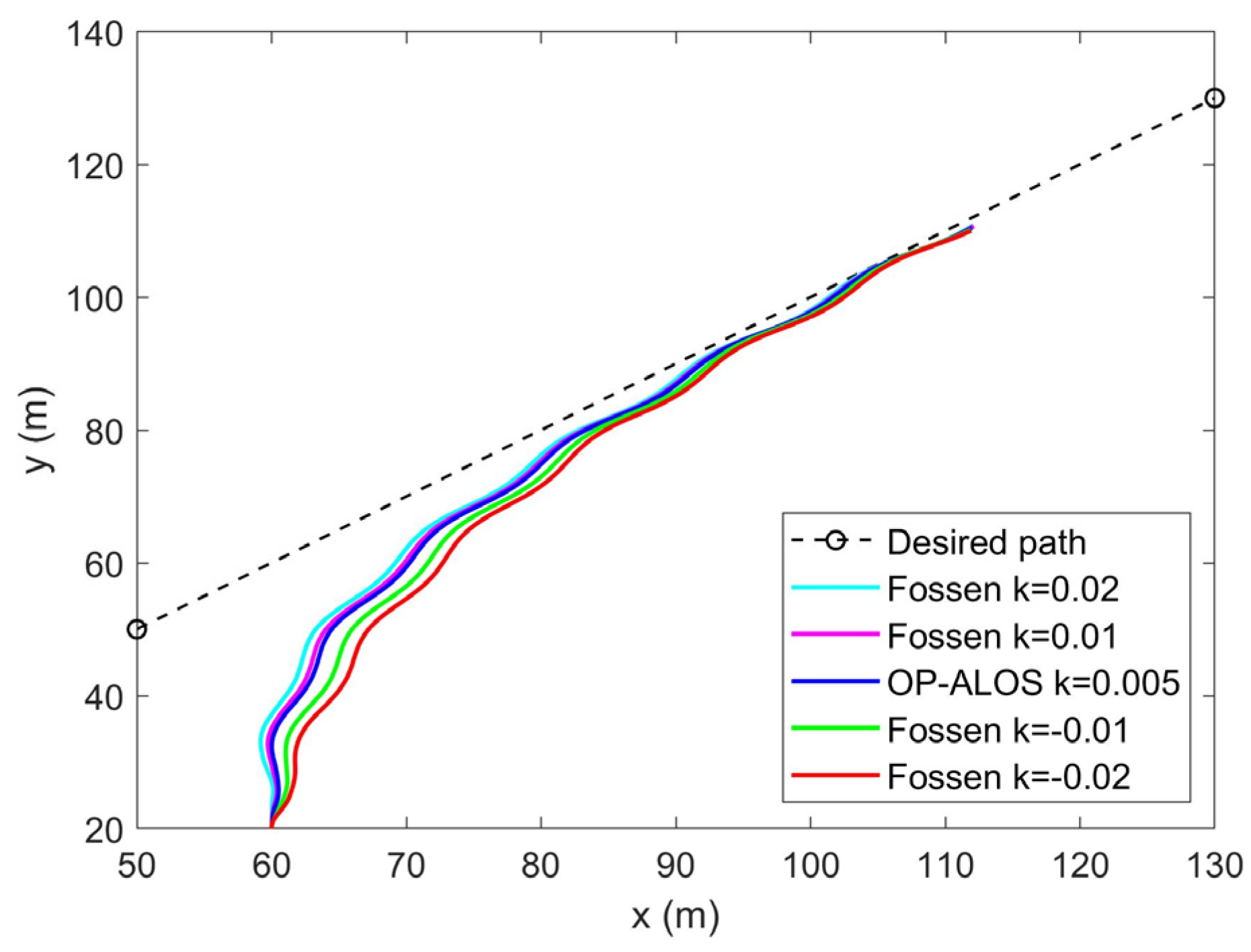
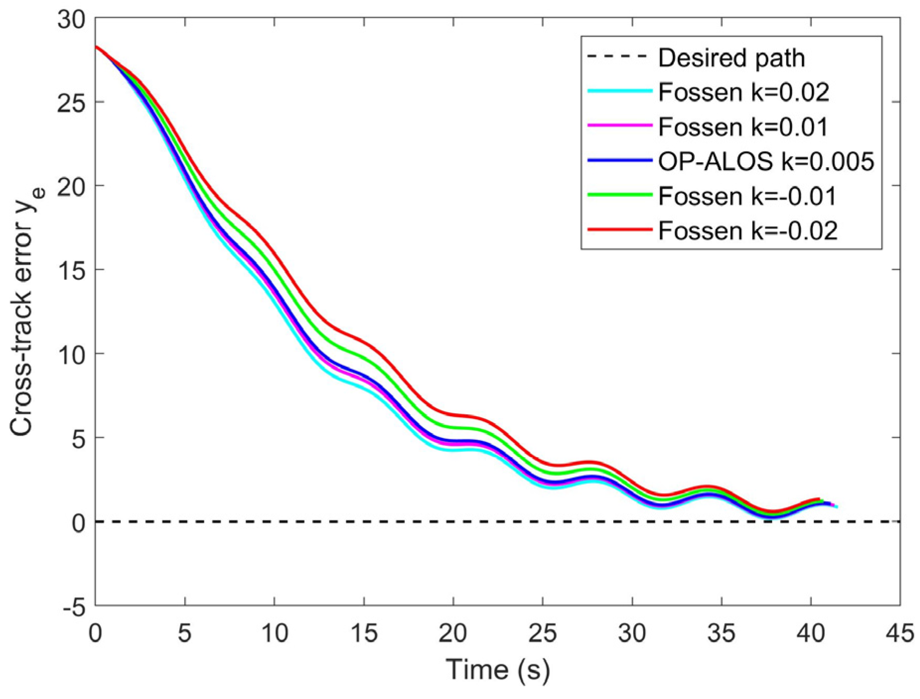
The parameters of ALOS need to be selected based on the motion model and control algorithm of the USV. The data of the USV in the simulation is shown in

Table 5. The data of the USV.

The Data of the USV	Value
Mass	$m=200\mathrm{kg}$
Length	$L=3.3\mathrm{m}$
Width	$B=1.5\mathrm{m}$
Sea water density	$\rho =1025\mathrm{kg}/{\mathrm{m}}^3$
Distance between thrusters	$l=0\mathrm{m}$ (Single thruster)
Propeller diameter	$D_p=0.235 \mathrm{m}$
Propeller speed	$n=900\mathrm{rpm}$
Rudder angle	$\delta \in \left[-15°,15°\right]$
Rudder rate	$\dot{\delta }\in \left[-5°/\mathrm{s}, 5°/\mathrm{s}\right]$

.

The simplified dynamic model of the USV [32] is established in (13). The mass matrix parameters of the USV can be obtained as follows: $m_{11}=210$, $m_{22}=264.29$, and $m_{33}=277.34$. The damping matrix parameters of the USV after interpolation and adjustment are as follows: $d_{11}=70.15$, $d_{22}=100$, and $d_{33}=284.30$.

$$\left\{\begin{array}{l}\dot{u}={\displaystyle \frac{m_{22}}{m_{11}}}vr-{\displaystyle \frac{d_{11}}{m_{11}}}u+{\displaystyle \frac{1}{m_{11}}}{\tau }_u\\ \dot{v}={\displaystyle \frac{m_{11}}{m_{22}}}ur-{\displaystyle \frac{d_{22}}{m_{22}}}v\\ \dot{r}={\displaystyle \frac{m_{11}-m_{22}}{m_{33}}}uv-{\displaystyle \frac{d_{33}}{m_{33}}}r+{\displaystyle \frac{1}{m_{11}}}{\tau }_r\end{array}\right.$$

(13)

The thrust generated by the thruster is based on the reference of the Wageningen B-Screw Series [33] according to the propeller speed. The thrust of the USV in each direction [34] is shown in (14), where $x_l=L/2$.

$$\left\{\begin{array}{l}{\tau }_u=Tcos\delta \\ {\tau }_v=Tsin\delta \\ {\tau }_r=x_{l}Tcos\delta \end{array}\right.$$

(14)

The initial speed of the USV is 1 m/s. In the LOS, ${\mathsf{\Delta }}_{\max }$ and ${\mathsf{\Delta }}_{\min }$ are set to 6 times and 3 times the length of the USV, respectively. The control algorithm for USV is PID, with the input of $y_e$ and the output of the rudder angle $\delta$. The relevant parameters are $k_p=8.35$, $k_i=0$, and $k_d=4.9$.

The key parameters for the Simulated Annealing algorithm are as follows: the initial temperature is 100; the final temperature is ${10}^{-8}$; and the random function is a standard normal distribution; the mean is 0; the standard deviation is 0.1; the initial solution is 0.01; the attenuation coefficient is 0.95; and the maximum iteration is 1000. The weight function $f_w$ is designed as shown in (15).

$$y_w=f_w\left(t_c,e_{max}\right)=a{e}_{max}+\left(1-a\right)t_c/10$$

(15)

(1)

Trajectory and cross-track error of the straight desired path

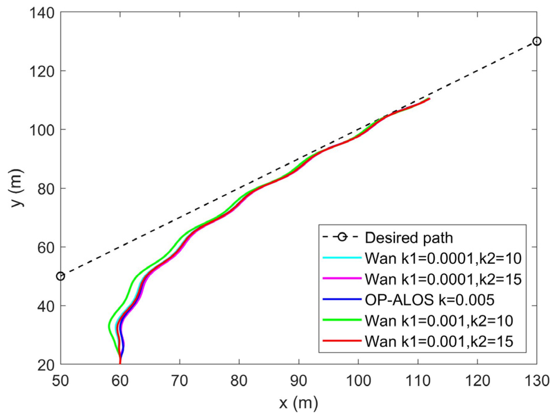
In the simulation of the straight desired path, the initial position $P_u$ is $\left(60,20\right)$. The points of the desired path (DP) are $P_{ki}=\left(50,50\right)$ and $P_{ki+1}=\left(130,130\right)$. We add the lateral time-varying disturbance velocity $\left(\sin t\right)\left(\sin 5°\right)U$, where $U$ is the speed of the USV and $t$ is the simulation time. The comparison results between ALOS with the optimized parameter (OP-ALOS) and guidance algorithms of Fossen and Wan are shown in Figure 48, Figure 49, Figure 50 and Figure 51.

Due to significant time-varying disturbances, the cross-track errors of USVs have not remained stable, and the corresponding stability errors and convergence time are invalid. The maximum errors corresponding to the five trajectories of OP-ALOS and Fossen’s algorithm are 0.1659, 0.2349, 0.2757, 0.4392, and 0.6001, with relatively small differences. The maximum errors corresponding to the five trajectories of OP-ALOS and Wan’s algorithm are 0.2871, 0.3186, 0.2757, 0.2121, and 0.2966. All maximum errors are positive, indicating that the USV is always on the same side as the start point relative to the desired path. The maximum error of OP-ALOS is 0.2757, which is relatively small, proving its effectiveness in time-varying disturbances.

(2)

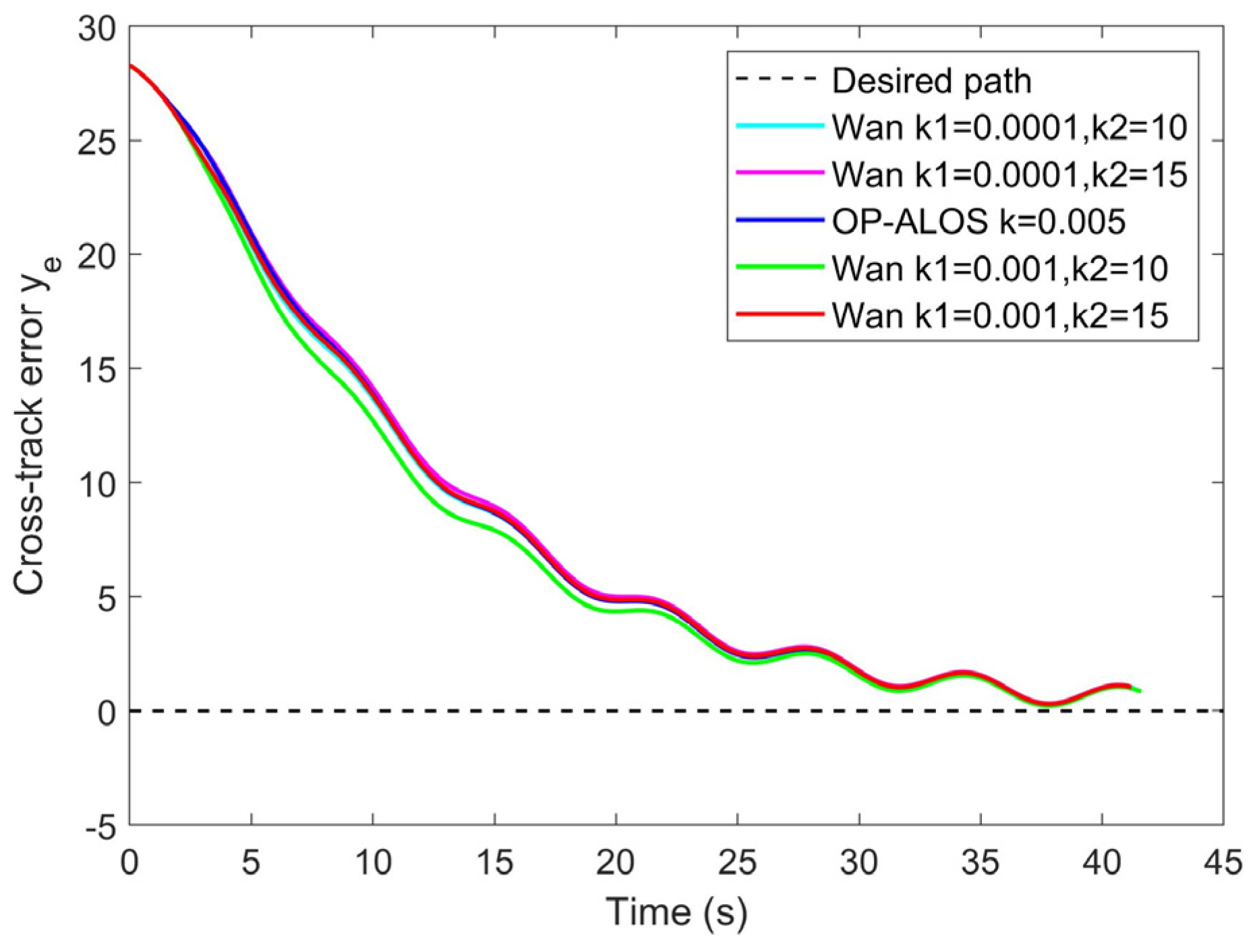
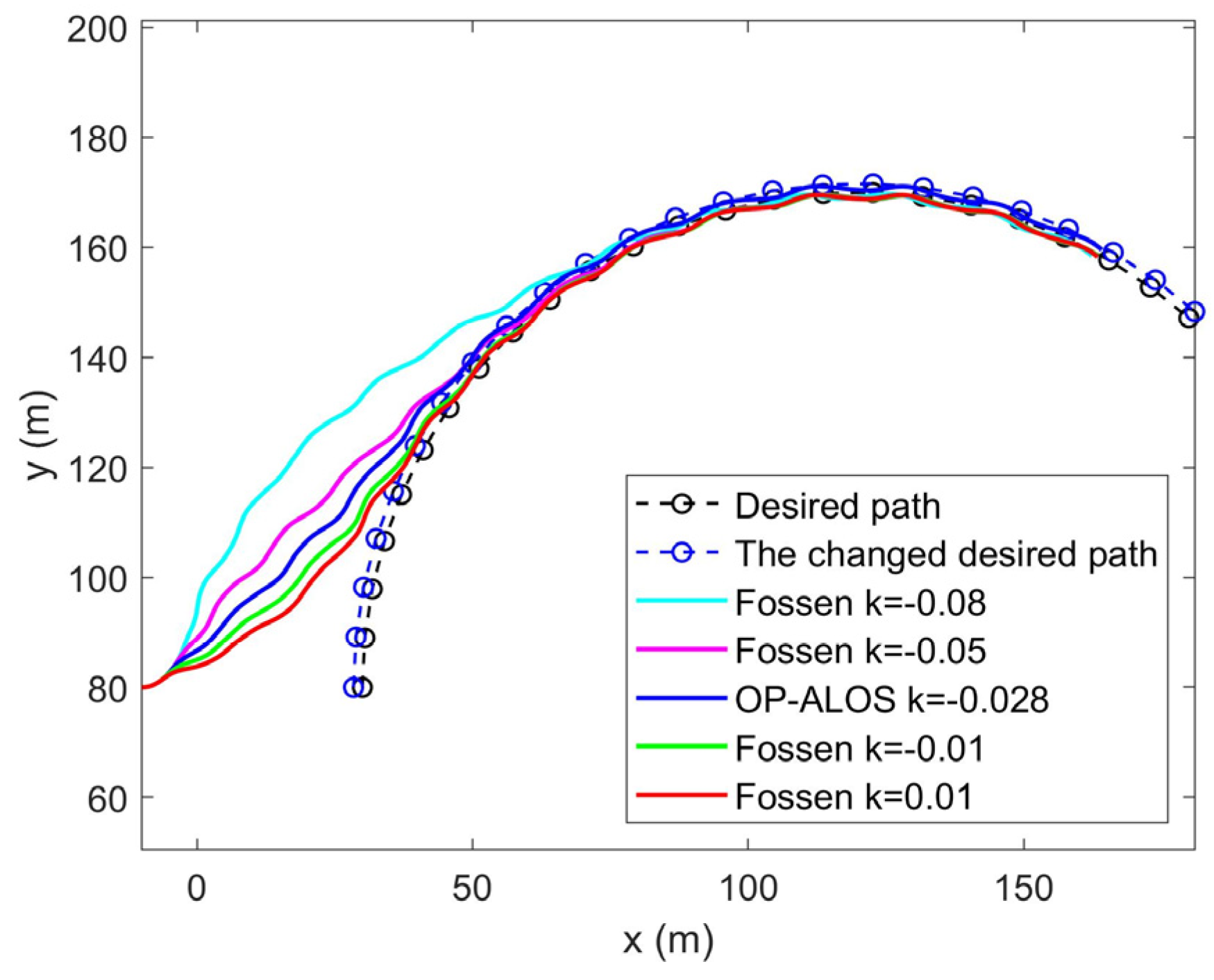
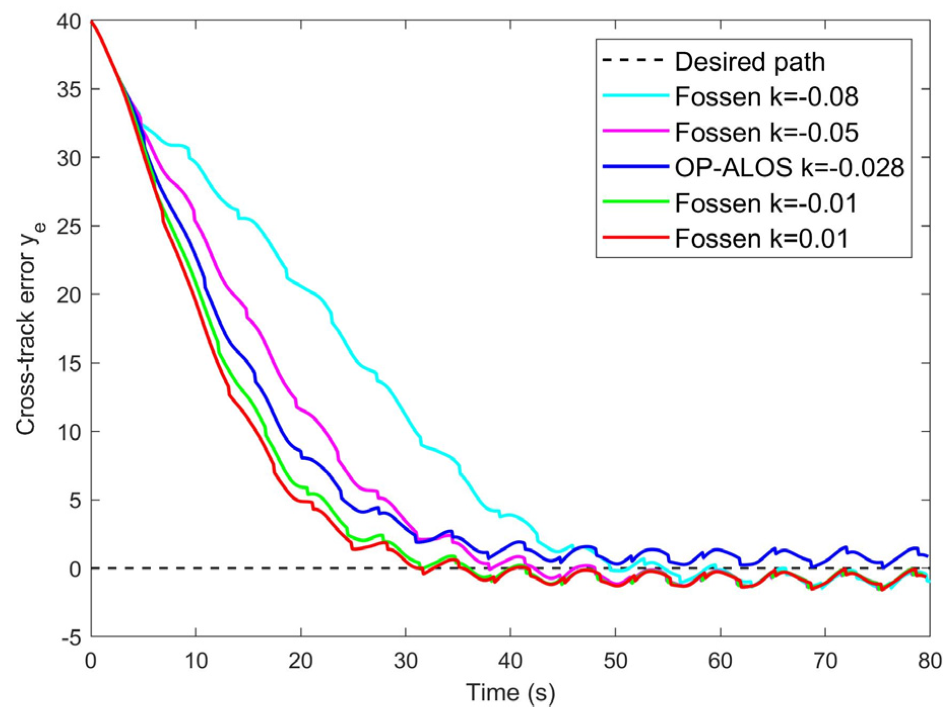
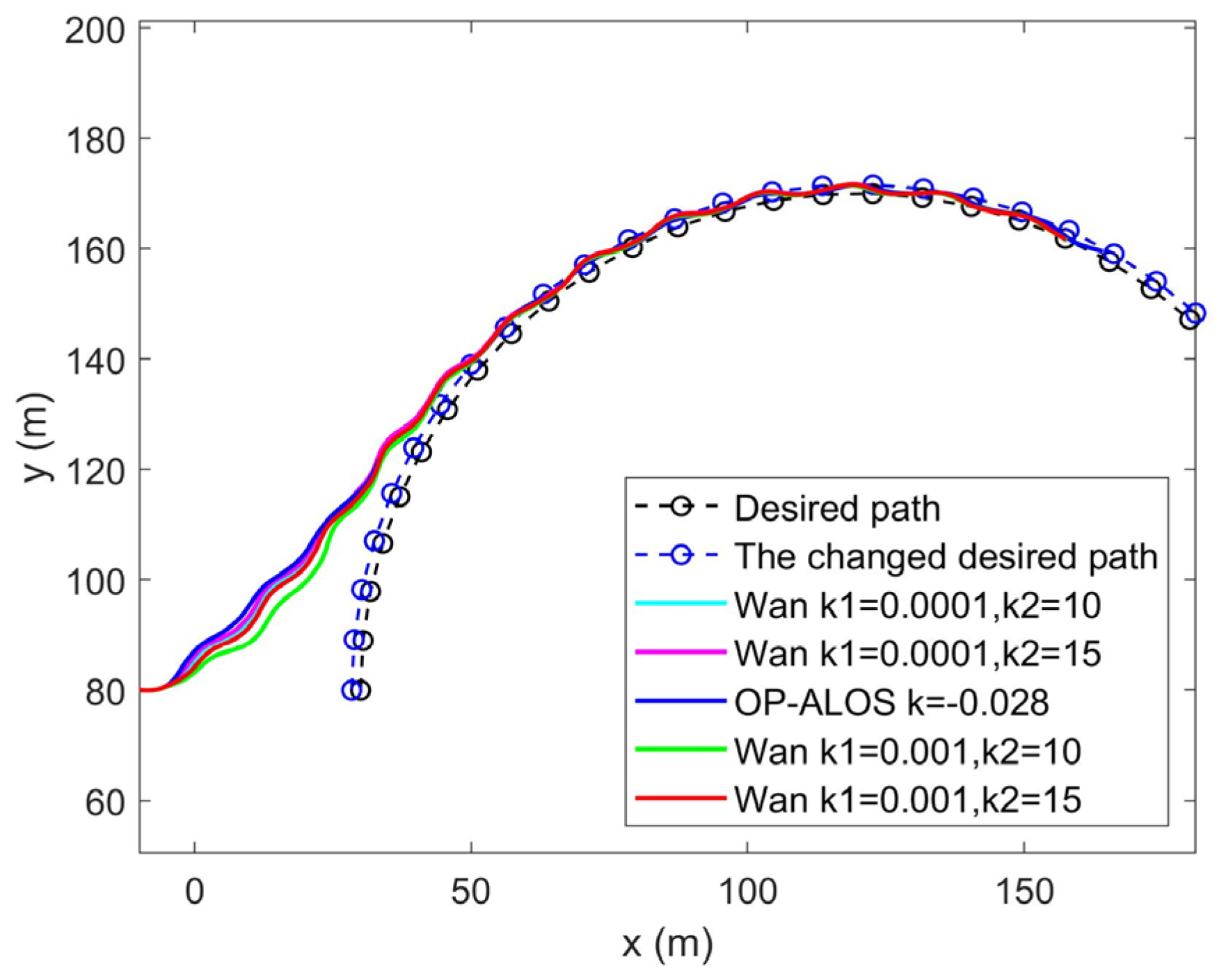
Trajectory and cross-track error of the curve desired path

In the simulation of the curve desired path, the comparison results between ALOS with the optimized parameter (OP-ALOS) and guidance algorithms of Fossen and Wan are shown in Figure 52, Figure 53, Figure 54 and Figure 55.

Due to significant time-varying disturbances, the trajectory errors of USVs have not remained stable, and the corresponding stability errors and convergence time are invalid. The maximum errors corresponding to the five trajectories of OP-ALOS and Fossen’s algorithm are −1.4597, −1.5166, 0.0110, −1.5332, and −1.5763, with relatively small differences. The maximum errors corresponding to the five trajectories of OP-ALOS and Wan’s algorithm are −0.1291, −0.1301, 0.0110, −0.1897, and −0.1613. Among them, the four maximum errors are all negative, indicating that the USV is always on the opposite side of the desired path from the start point, which is more dangerous. The maximum error of OP-ALOS is 0.0110, with a relatively small absolute value, which proves the effectiveness of the optimized guidance algorithm in time-varying disturbances.

5. Conclusions

In this paper, LCPP is proposed as a low-complexity path-planning algorithm for multiple USVs based on the visibility graph method. While ensuring a shorter path distance, the algorithm outperforms the comparison algorithm in terms of computational complexity, reducing the original path planning computational $O\left(n^2\right)$ complexity to $O\left(n\right)$. When the number of USVs is large, the LCPP algorithm requires less calculation time and maintains a shorter path distance. OP-ALOS is proposed as an algorithm of ALOS with optimized parameters to ensure the USV approaches obstacle edges quickly and maintains a specific safe distance from the obstacles. Even in time-varying disturbances, this algorithm can also reduce the maximum error. The effectiveness of the algorithm has been verified through simulation. In addition, this algorithm can only be used in static and known environments. In the future, we will investigate more USVs working together to explore unknown environments and reach target points.

References

1. Salima, B.; Assia, B.; Ghalem, B. HA-UVC: Hybrid approach for unmanned vehicles cooperation. Multiagent Grid Syst. 2020, 16, 1–45. [Google Scholar] [CrossRef]
2. Zhong, J.B.; Li, B.Y.; Li, S.X.; Yang, F.; Li, P.; Cui, Y. Particle swarm optimization with orientation angle-based grouping for practical unmanned surface vehicle path planning. Appl. Ocean Res. 2021, 111, 102658. [Google Scholar] [CrossRef]
3. Dvorak, M.; Dolezel, P.; Stursa, D.; Chouai, M. Genetic Algorithm-Based Task Assignment for Fleet of Unmanned Surface Vehicles in Dynamically Changing Environment. Cybern. Syst. 2023, 55, 1314–1331. [Google Scholar] [CrossRef]
4. Zwolak, K.; Wigley, R.; Bohan, A.; Zarayskaya, Y.; Bazhenova, E.; Dorshow, W.; Sumiyoshi, M.; Sattiabaruth, S.; Roperez, J.; Proctor, A.; et al. The Autonomous Underwater Vehicle Integrated with the Unmanned Surface Vessel Mapping the Southern Ionian Sea. The Winning Technology Solution of the Shell Ocean Discovery XPRIZE. Remote Sens. 2020, 12, 1344. [Google Scholar] [CrossRef]
5. Wu, G.X.; Xu, T.T.; Sun, Y.S.; Zhang, J. Review of multiple unmanned surface vessels collaborative search and hunting based on swarm intelligence. Int. J. Adv. Robot. Syst. 2022, 19, 17298806221091885. [Google Scholar] [CrossRef]
6. Xing, B.W.; Yu, M.J.; Liu, Z.C.; Tan, Y.; Sun, Y.; Li, B. A Review of Path Planning for Unmanned Surface Vehicles. J. Mar. Sci. Eng. 2023, 11, 1556. [Google Scholar] [CrossRef]
7. Liu, Y.C.; Bucknall, R. Efficient multi-task allocation and path planning for unmanned surface vehicle in support of ocean operations. Neurocomputing 2018, 275, 1550–1566. [Google Scholar] [CrossRef]
8. Chen, X.Y.; Zhang, P.; Du, G.L.; Li, F. Ant Colony Optimization Based Memetic Algorithm to Solve Bi-Objective Multiple Traveling Salesmen Problem for Multi-Robot Systems. IEEE Access 2018, 6, 21745–21757. [Google Scholar] [CrossRef]
9. Liu, Y.C.; Song, R.; Bucknall, R.; Zhang, X. Intelligent multi-task allocation and planning for multiple unmanned surface vehicles (USVs) using self-organising maps and fast marching method. Inf. Sci. 2019, 496, 180–197. [Google Scholar] [CrossRef]
10. Ning, Q.; Tao, G.P.; Chen, B.C.; Lei, Y.; Yan, H.; Zhao, C. Multi-UAVs trajectory and mission cooperative planning based on the Markov model. Phys. Commun. 2019, 35, 100717. [Google Scholar] [CrossRef]
11. Lusk, P.C.; Cai, X.Y.; Wadhwania, S.; Paris, A.; Fathian, K.; How, J.P. A Distributed Pipeline for Scalable, Deconflicted Formation Flying. IEEE Robot. Autom. Lett. 2020, 5, 5213–5220. [Google Scholar] [CrossRef]
12. Xia, G.Q.; Sun, X.X.; Xia, X.M. Multiple Task Assignment and Path Planning of a Multiple Unmanned Surface Vehicles System Based on Improved Self-Organizing Mapping and Improved Genetic Algorithm. J. Mar. Sci. Eng. 2021, 9, 556. [Google Scholar] [CrossRef]
13. Ma, Y.; Zhao, Y.J.; Li, Z.X.; Bi, H.; Wang, J.; Malekian, R.; Sotelo, M.A. CCIBA*: An Improved BA* Based Collaborative Coverage Path Planning Method for Multiple Unmanned Surface Mapping Vehicles. IEEE Trans. Intell. Transp. Syst. 2022, 23, 19578–19588. [Google Scholar] [CrossRef]
14. Zhao, Z.Y.; Zhu, B.; Zhou, Y.; Yao, P.; Yu, J. Cooperative Path Planning of Multiple Unmanned Surface Vehicles for Search and Coverage Task. Drones 2023, 7, 21. [Google Scholar] [CrossRef]
15. Yao, P.; Wu, K.Q.; Lou, Y.T. Path Planning for Multiple Unmanned Surface Vehicles Using Glasius Bio-Inspired Neural Network With Hungarian Algorithm. IEEE Syst. J. 2022, 17, 3906–3917. [Google Scholar] [CrossRef]
16. Yu, J.B.; Chen, Z.H.; Zhao, Z.Y.; Yao, P.; Xu, J. A traversal multi-target path planning method for multi-unmanned surface vessels in space-varying ocean current. Ocean Eng. 2023, 278, 114423. [Google Scholar] [CrossRef]
17. Pei, M.; An, H.; Liu, B.; Wang, C. An Improved Dyna-Q Algorithm for Mobile Robot Path Planning in Unknown Dynamic Environment. IEEE Trans. Syst. Man Cybern. Syst. 2022, 52, 4415–4425. [Google Scholar] [CrossRef]
18. Zhang, J. Path Planning for a Mobile Robot in Unknown Dynamic Environments Using Integrated Environment Representation and Reinforcement Learning. In Proceedings of the 2019 Australian & New Zealand Control Conference (ANZCC), Auckland, New Zealand, 27–29 November 2019; pp. 258–263. [Google Scholar]
19. Wu, K.; Wang, H.; Esfahani, M.A.; Yuan, S. Achieving Real-Time Path Planning in Unknown Environments Through Deep Neural Networks. IEEE Trans. Intell. Transp. Syst. 2022, 23, 2093–2102. [Google Scholar] [CrossRef]
20. Qin, Y.M.; Liu, J.X.; Shao, X.; Duan, S. Rapid path planning for Unmanned Surface Vessels. In Proceedings of the SPIE 11th International Symposium on Multispectral Image Processing and Pattern Recognition (MIPPR)—Remote Sensing Image Processing, Geographic Information Systems, and Other Applications, 2019, Wuhan, China, 14 February 2020; Volume 11432, pp. 279–285. [Google Scholar]
21. Lozano-Pérez, T.; Wesley, M.A. An Algorithm for Planning Collision Free Paths Among Polyhedral Obstacles. Commun. ACM 1979, 22, 560–570. [Google Scholar] [CrossRef]
22. Lekkas, A.M.; Fossen, T.I. Line-of-Sight Guidance for Path Following of Marine Vehicles. Adv. Mar. Robot. 2013, 5, 63–92. [Google Scholar]
23. Fossen, T.I. Handbook of Marine Craft Hydrodynamics and Motion Control. Guidance Systems; John Wiley & Sons: Hoboken, NJ, USA, 2011; pp. 240–284. [Google Scholar]
24. Lekkas, A.M.; Fossen, T.I. Integral LOS Path Following for Curved Paths Based on a Monotone Cubic Hermite Spline Parametrization. IEEE Trans. Control. Syst. Technol. 2014, 22, 2287–2301. [Google Scholar] [CrossRef]
25. Fossen, T.I.; Pettersen, K.Y. On uniform semiglobal exponential stability (USGES) of proportional line-of-sight guidance laws. Automatica 2014, 50, 2912–2917. [Google Scholar] [CrossRef]
26. Liu, L.S.; Wang, B.; Xu, H. Research on Path-Planning Algorithm Integrating Optimization A-Star Algorithm and Artificial Potential Field Method. Electronics 2022, 11, 3660. [Google Scholar] [CrossRef]
27. Zhang, Z.; Wu, D.F.; Gu, J.D.; Li, F. A Path-Planning Strategy for Unmanned Surface Vehicles Based on an Adaptive Hybrid Dynamic Stepsize and Target Attractive Force-RRT Algorithm. J. Mar. Sci. Eng. 2019, 7, 132. [Google Scholar] [CrossRef]
28. Zhang, Z.C.; Wu, H.B.; Zhou, H.; Song, Y.; Chen, Y.; He, K.; Gao, J. Recovery Path Planning for Autonomous Underwater Vehicles Using Constrained Bi-RRT*-Smart Algorithms. In Proceedings of the OCEANS Conference, Limerick, Ireland, 5–8 June 2023. [Google Scholar]
29. Liu, C.Y.; Xie, S.B.; Sui, X.; Huang, Y.; Ma, X.; Guo, N.; Yang, F. PRM-D* Method for Mobile Robot Path Planning. Sensors 2023, 23, 3512. [Google Scholar] [CrossRef] [PubMed]
30. Mustafa, Y.A.; Ali, E.S.; Osman, T.E.; Khalifa, O.O.; Mohamed, Z.O.; Saeed, R.A.; Saeed, M.M. Multi-Drones Energy Efficient Based Path Planning Optimization using Genetic Algorithm and Gradient Decent Approach. In Proceedings of the 9th International Conference on Mechatronics Engineering (ICOM), Kuala Lumpur, Malaysia, 13–14 August 2024; pp. 171–176. [Google Scholar]
31. Hu, J.H.; Er, M.J.; Liu, T.H.; Wang, S. A Hybrid Algorithm Based on Ant Colony and Genetic Algorithm for AUV Path Planning. In Proceedings of the 2nd Conference on Fully Actuated System Theory and Applications (CFASTA), Qingdao, China, 14–16 July 2023; pp. 888–893. [Google Scholar]
32. Mu, D.; Wang, G.; Fan, Y.; Sun, X.; Qiu, B. Modeling and Identification for Vector Propulsion of an Unmanned Surface Vehicle: Three Degrees of Freedom Model and Response Model. Sensors 2018, 18, 1889. [Google Scholar] [CrossRef]
33. Helma, S. Surprising Behaviour of the Wageningen B-Screw Series Polynomials. J. Mar. Sci. Eng. 2020, 8, 211. [Google Scholar] [CrossRef]
34. Faramin, M.; Goudarzi, R.H.; Maleki, A. Track-keeping observer-based robust adaptive control of an unmanned surface vessel by applying a 4-DOF maneuvering model. Ocean Eng. 2019, 183, 11–23. [Google Scholar] [CrossRef]
Figure 1. The USV turning.
Jmse 13 00556 g001
Figure 2. Obstacle and safe distance.
Jmse 13 00556 g002
Figure 3. The flow chart for the algorithms.
Jmse 13 00556 g003
Figure 4. Example of VG.
Jmse 13 00556 g004
Figure 5. Obstacle and safe distance.
Jmse 13 00556 g005
Figure 6. Initial state.
Jmse 13 00556 g006
Figure 7. Filter and discover optional paths.
Jmse 13 00556 g007
Figure 8. Filter but no optional path found.
Jmse 13 00556 g008
Figure 9. The result of filtering optional paths.
Jmse 13 00556 g009
Figure 10. Filter and discover optional paths.
Jmse 13 00556 g010
Figure 11. The result of filtering optional paths.
Jmse 13 00556 g011
Figure 12. Start point, target point, and obstacles.
Jmse 13 00556 g012
Figure 13. Calculation results of VG.
Jmse 13 00556 g013
Figure 14. Safety boundary of obstacles.
Jmse 13 00556 g014
Figure 15. Possible paths from the start point.
Jmse 13 00556 g015
Figure 16. The filtered path from the start point.
Jmse 13 00556 g016
Figure 17. Possible paths from the target point.
Jmse 13 00556 g017
Figure 18. The filtered path from the target point.
Jmse 13 00556 g018
Figure 19. Calculation results of LCPP.
Jmse 13 00556 g019
Figure 20. The path to be calculated.
Jmse 13 00556 g020
Figure 21. The result of the Dijkstra algorithm once.
Jmse 13 00556 g021
Figure 22. All paths start from start point 1.
Jmse 13 00556 g022
Figure 23. All paths start from start point 2.
Jmse 13 00556 g023
Figure 24. All paths start from start point 3.
Jmse 13 00556 g024
Figure 25. All paths start from start point 4.
Jmse 13 00556 g025
Figure 26. LOS guidance law.
Jmse 13 00556 g026
Figure 27. Evaluation parameters of LOS.
Jmse 13 00556 g027
Figure 28. Change in the desired path to reduce the steady-state error.
Jmse 13 00556 g028
Figure 29. Simulation area.
Jmse 13 00556 g029
Figure 30. Planning path using LCPP.
Jmse 13 00556 g030
Figure 31. Initial map of A*1.
Jmse 13 00556 g031
Figure 32. Path planning using A*1.
Jmse 13 00556 g032
Figure 33. Path planning using A*2.
Jmse 13 00556 g033
Figure 34. Path planning using A*3.
Jmse 13 00556 g034
Figure 35. Building a potential field using FMM.
Jmse 13 00556 g035
Figure 36. Path planning using FMM.
Jmse 13 00556 g036
Figure 37. Explore maps using RRT.
Jmse 13 00556 g037
Figure 38. Path planning using RRT.
Jmse 13 00556 g038
Figure 39. Explore maps using Bi-RRT.
Jmse 13 00556 g039
Figure 40. Path planning using Bi-RRT.
Jmse 13 00556 g040
Figure 41. Explore maps using PRM.
Jmse 13 00556 g041
Figure 42. Path planning using PRM.
Jmse 13 00556 g042
Figure 43. Path planning using GA/GD.
Jmse 13 00556 g043
Figure 44. Path planning using ACO.
Jmse 13 00556 g044
Figure 45. Calculation time of 10 algorithms.
Jmse 13 00556 g045
Figure 46. Calculation time of 5 algorithms.
Jmse 13 00556 g046
Figure 47. The average path length of 10 algorithms.
Jmse 13 00556 g047
Figure 48. Comparison of trajectory with Fossen’s algorithm.
Jmse 13 00556 g048
Figure 49. Comparison of cross-track error with Fossen’s algorithm.
Jmse 13 00556 g049
Figure 50. Comparison of trajectory with Wan’s algorithm.
Jmse 13 00556 g050
Figure 51. Comparison of cross-track error with Wan’s algorithm.
Jmse 13 00556 g051
Figure 52. Comparison of trajectory with Fossen’s algorithm.
Jmse 13 00556 g052
Figure 53. Comparison of cross-track error with Fossen’s algorithm.
Jmse 13 00556 g053
Figure 54. Comparison of trajectory with Wan’s algorithm.
Jmse 13 00556 g054
Figure 55. Comparison of cross-track error with Wan’s algorithm.
Jmse 13 00556 g055