Abstract
Ensuring safety and preventing accidents in waterway channels are critical challenges for networked marine surface vessel systems (NMSVs). This study introduces a regulation-aware decision-making system designed to minimize traffic conflicts and enhance navigational safety in inland waterway traffic separation schemes. The proposed framework integrates a hierarchical conditional state machine with chance-constrained model predictive control, allowing NMSVs to handle complex traffic situations while complying with safety regulations. The hierarchical conditional state machine effectively identifies vessel maneuver states, implementing safety constraints that proactively avoid collisions. Meanwhile, the chance-constrained model predictive control optimizes vessel trajectories, factoring in uncertainties and potential risks, while simultaneously enhancing operational efficiency. Simulation and experimental results demonstrate that the proposed system significantly reduces the likelihood of accidents and improves overall safety by efficiently managing vessel interactions. Compared to traditional methods, the regulation-aware approach ensures better collision avoidance, greater regulation compliance, and superior safety performance. This study confirms that the proposed decision-making system can be effectively implemented in real time, offering practical benefits for improving waterway safety and mitigating accident risks.
1. Introduction
Maritime transportation plays a crucial role in the global transportation system, with the shipping industry continuously striving to enhance operational efficiency, vessel intelligence, and navigation safety [1]. Currently, ship navigation heavily depends on onboard communication and navigation systems, which offer limited capabilities in terms of navigation information and communication. This constraint hampers the timely, comprehensive, and effective utilization of available information resources, resulting in a shortage of critical data and hindering the realization of full interconnectivity. Consequently, this leads to inadequate security risk mitigation. Additionally, the absence of an efficient ship navigation system results in low communication efficiency between vessels and ports, further exacerbating the risk of accidents and incidents, such as delays in departures and arrivals, ship collisions, and groundings [2].
To address these challenges within the maritime sector, our research team previously proposed the Internet of Ships (IoS) conceptual framework. Building upon the IoS framework, this paper introduces a novel behavior planning framework aimed at ensuring both the safety of ship navigation and the efficient coordination of vessels. Ensuring the safety of networked marine surface vessel systems (NMSVs) in inland waterway channels is of paramount importance to preventing maritime accidents and minimizing traffic conflicts. Collisions between vessels, especially in constrained waterway environments, pose significant risks not only to human life but also to the environment and economy [3]. Ensuring that NMSVs comply with both safety regulations and navigational rules is paramount to preventing such incidents and ensuring efficient waterway traffic management [4]. NMSVs are increasingly recognized as vital components of modern maritime navigation, enabling fully autonomous operations while mitigating the risks associated with human error [5]. Therefore, it is essential to develop intelligent decision-making and motion planning systems that can mitigate these risks, enhance operational safety, and ensure compliance with maritime regulations.
Autonomous navigation for NHMSVs typically involves three core components: perception, decision-making/planning, and control. These systems must operate in complex environments with dynamic traffic conditions, where the behavior of surrounding vessels can change unpredictably [6]. To ensure safe navigation, it is crucial for NMSVs to not only detect obstacles but also predict their movements, assess the traffic situation, and make real-time decisions that reduce the likelihood of accidents.
Navigating through narrow waterway channels, especially in mixed traffic environments involving both NMSVs and human-operated vessels, presents significant challenges. The absence of fixed traffic lanes and traffic signals on the water creates an inherently dynamic environment that requires careful coordination to avoid collisions. These challenges are further compounded by the need to adhere to global maritime safety regulations, such as the International Regulations for Preventing Collisions at Sea (COLREGs), which govern the movement of vessels in constrained spaces.
When faced with these complex dynamics, automated decision-making systems play a pivotal role in NMSVs’ ability to navigate safely and efficiently. These systems must evaluate the surrounding environment in real time and make decisions that reduce the risk of collisions, account for uncertainties, and ensure adherence to maritime regulations [7]. NMSV behavioral decision-making strategies can generally be classified into rule-based systems [8] and learning-based approaches [9]. While rule-based systems rely on predefined conditions and regulations, learning-based methods can adapt to dynamic conditions and optimize decision-making through continuous feedback.
A decision-making system evaluates the surrounding environment and determines the vessel’s behaviors [10] based on the available options and resource constraints. Kim proposed an autonomous intelligent body architecture approach to solve the optimal task planning problem for vessels [11]. This approach has some advantages owing to its highly autonomous multi-subject architecture features capable of performing state estimation, maintaining environment awareness, determining the task goal, planning/re-planning to achieve the set goal, and allocating resources. Ferris proposed a scalable mission planning architecture that allows vessels to reach multiple target points with time-optimal mission plans [12]. The vessel’s route planning is seen as a mass. The vessel is considered a non-holonomic constrained vessel in trajectory planning, considering kinematic constraints. Finally, dynamical constraints are introduced to motion planning, fully considering the behavioral constraints (rules) and the vessel’s dynamic information.
Planning is a multi-scale constraint problem, typically applied to large-scale scenarios, treating the object of research as a particle with no dynamic properties. Vessel behavior planning [13] relates to vessel navigation, consisting of behavior, task, and motion planning [14]. However, the navigation of waterway channels presents difficulties in terms of motion planning due to the constrained space available and the presence of other vessels driven by humans. Collisions between ships are a severe danger to maritime safety, and particular care should be taken with the ship’s operation in narrow channels to avoid accidents, substantial economic losses, and environmental destruction [3]. Furthermore, it is important to note that an accident has the potential to result in insignificant economic ramifications due to the subsequent disruption of key transportation routes.
The successful navigation of waterways necessitates meticulous preparation and precise execution to circumvent potential collisions with both stationary and moving impediments. Furthermore, adherence to interaction regulations [15] in canal channels is of utmost importance, akin to the collision avoidance laws at sea (COLREGs) [16]. The adherence to these restrictions is obligatory, and by doing so, the movements of the NMSV become socially compliant and predictable to other individuals utilizing the canal.
While NMSVs and other autonomous vehicles [17] have been studied in dynamic environments, motion planning for NMSVs faces unique challenges due to the special environment in inland waterway traffic separation schemes. Unlike road-based autonomous vehicles, NMSVs must navigate without predefined lanes or traffic signals, and their motion planning must take into account both their own physical dynamics and the potential behavior of nearby vessels [18]. Furthermore, unlike mobile robots navigating unstructured environments [19], NMSVs must also comply with maritime-specific traffic regulations to ensure safe passage [20]. Wang et al. proposed an algorithm for avoiding collisions, allowing virtual lanes to run parallel to waterways [21]. Tao et al. [4] produced a plan for channels to be followed by the vessel train model. However, these studies failed to consider avoidance regulations in the waterway channel, including interaction regulations, which consider ships’ operation in channels.
Current approaches to collision avoidance in waterway navigation often fail to fully incorporate the need for regulation-aware decision-making, particularly regarding interaction rules, which govern vessel operation in constrained channels [22]. While previous studies have proposed various strategies for collision avoidance, many have overlooked the importance of considering waterway-specific regulations, such as the guidelines for safe operation in narrow channels and the interactions between vessels. These regulations are crucial for preventing accidents, yet they are often inadequately integrated into existing motion planning systems. Many studies have explored different methods for autonomous vessel navigation, focusing primarily on optimizing decision-making processes. Model predictive control (MPC) has been one of the most widely applied techniques due to its ability to handle multiple variables and constraints while optimizing vessel trajectories in real time. For instance, MPC has shown promising results in collision avoidance in maritime traffic. However, one of the main limitations of traditional MPC approaches lies in real-time decision-making. The computational complexity involved in solving optimization problems in high-traffic conditions often prevents these methods from operating effectively in real time, particularly when high-density traffic or unpredictable environmental factors are involved.
On the other hand, reinforcement learning methods have emerged as a potential solution to dynamic decision-making, as they can adapt to the environment over time. However, these methods face challenges in terms of scalability and the need for large datasets. Moreover, reinforcement learning does not inherently provide guarantees for regulatory compliance or safety, which are essential in maritime contexts where collision avoidance and traffic regulations are crucial.
Although several advances have been made, these methods still have limitations in scalability and real-time applicability, especially in inland waterways, where high-traffic conditions and environmental factors add additional layers of complexity.
To address the existing challenges in maritime safety and navigation efficiency, we propose a novel approach that integrates hierarchical conditional state machine (HCSM) and chance-constrained model predictive control (CC-MPC). Our approach specifically addresses the limitations of traditional methods, offering a solution that is scalable, feasible in real time, and capable of handling uncertainties in dynamic, high-density environments. The combination of HCSM and CC-MPC allows for safe and efficient navigation of vessels, ensuring collision avoidance, compliance with traffic regulations, and adaptability to unforeseen circumstances, such as changes in traffic patterns or environmental factors. This combination enables dynamic decision-making while ensuring the system remains computationally efficient enough for real-time operation.
The proposed framework integrates hierarchical conditional state machines with chance-constrained model predictive control. This hybrid approach enables vessels to navigate complex traffic scenarios while adhering to both safety constraints and traffic regulations. By leveraging the IoS infrastructure, our system allows for more effective decision-making and coordination. Furthermore, the use of edge computing allows for localized processing of real-time environmental data, reducing latency and enhancing the timeliness of decision-making in critical situations.
The key contributions of this paper are as follows:
- (1)
- This paper presents a novel regulation-aware decision-making framework that leverages the Internet of Ships and edge computing to integrate behavioral decision-making with motion planning, specifically designed to enhance the safety and efficiency of NMSVs operating in inland waterway channels.
- (2)
- Hierarchical conditional state machine is employed to make decisions about the vessel’s maneuvers based on the current traffic situation, implementing safety constraints to prevent collisions.
- (3)
- The chance-constrained model predictive Control is then used to optimize the vessel’s trajectory, factoring in both the vessel’s own dynamic constraints and the uncertainty in the surrounding traffic environment. This integrated approach not only enhances collision avoidance but also ensures that NMSVs adhere to traffic regulations, improving overall safety and reducing the potential for accidents.
The subsequent sections of this paper are structured in the following manner: Section 2 of this paper provides an overview of the theoretical background. Section 3 of the document focuses on the decision-making framework that governs the behavior of autonomous surface vehicles in waterway channels and the optimal planning approach utilizing a chance-constrained model prediction framework. Section 4 discusses case study. Section 5 summarizes the discussion and conclusions.
2. Problem Formulation
In the autonomous navigation phase, vessels must rely on the integrated system’s perception, decision-making, and execution capabilities to achieve autonomous control without the need for human intervention [23]. At this stage, the system must exhibit robust data processing, real-time decision-making, and incident response capabilities [24,25]. The above scenarios are the basis of the algorithm studied in this paper and are mentioned in our previous research [26].
2.1. Vessel Behavior Modeling
Understanding traffic separation schemes, as regulated by the International Maritime Organization (IMO), is crucial for preventing accidents and enhancing the safety of vessel operations in waterway channels. These schemes are designed to organize vessel movement, helping to mitigate the risk of collisions and improve traffic flow in congested or narrow waterways. Historically, traffic separation schemes typically involve dual-lane systems to guide vessels in distinct directions, but in inland waterways, the restricted width often necessitates single-lane configurations.
In dynamic environments, vessels frequently interact with other ships, and these interactions can range from benign to hazardous, directly influencing both the safety of the vessel in question and the overall traffic dynamics. The key to reducing accidents lies in understanding and modeling these interactions. Preliminary studies [13] indicate that the nature of ship-to-ship interactions—shaped by factors such as proximity, speed, and maneuvers—significantly impacts overall vessel behavior and collision risks.
In the context of waterway navigation, vessel behavior can be broken down into three critical stages: situational awareness, decision-making, and execution of maneuvers. Vessels must continuously assess the surrounding traffic conditions, gathering data from other vessels and evaluating potential risks to avoid accidents. These ongoing assessments help vessels to make real-time adjustments to their operations, including changes in heading or speed, based on the movement of other ships. These adjustments, however, often trigger ripple effects that can alter the overall traffic situation, potentially introducing new safety risks that must be mitigated.
The navigation status of a vessel includes serval-dimensional state sets composed of position information (east x and north y), vessel velocity v, heading angel c, vessel decision state d, vessel control input τ, and other dynamic attributes. The expression of a vessel’s navigation state in maritime traffic is as follows:
where is the timestamp, is the vessel behavior of vessel , n is the number of the vessel, and is the navigation status of the vessel at time .
Vessels must continuously adapt to changes in the navigation status of surrounding vessels. Significant variations in navigation status can lead to safety incidents, necessitating appropriate behavioral adjustments. This process entails perceiving environmental changes, deciding on navigational alterations, and executing actions to maintain safety. Recent advancements in traffic separation schemes, akin to highway lanes, have been implemented to enhance safety and prevent collisions. The interaction process of vessel behavior is classified into three stages: perceiving the traffic environment, assessing movement trends, and, if required, altering navigation states to avoid collisions. This tripartite approach ensures safe and efficient navigation, with vessels constantly evaluating traffic conditions and adjusting behaviors according to established rules and emerging safety threats.
Sailing routes are determined by ship captains over thousands of years of sailing practice. Then, waterways, known as the traffic separation scheme, gradually appeared like “lanes” on highways to prevent ships from colliding. The traffic separation scheme, regulated by the International Maritime Organization, is a route-management system for traffic management. Historically, a single traffic separation scheme consists of two lanes. A vessel sailing in a traffic lane should follow the approximate direction of that lane. Each vessel in the traffic separation scheme is assigned to one of three statuses. Once the vessel has entered the traffic separation scheme, it is able to navigate along its intended course and at the chosen velocity without any restrictions.
Nevertheless, if a target vessel travels at a slower velocity and is positioned ahead, it is possible for the vessel in question to utilize an adjacent lane to surpass the vessel, if there is minimal vehicular congestion in the opposing direction. The procedure is commonly referred to as vessel overtaking. Due to environmental indications or human factors, the vessel may encounter head-on situations in narrow channels during the sailing process. The vessel may observe transitioning between phases based on the current maritime conditions.
This study redefines vessel sailing behavior within the traffic separation scheme into two primary states: normal sailing and collision avoidance (as shown in Table 1). Collision avoidance is further subdivided into chasing and encountering scenarios, depending on the specific environmental and traffic conditions within the waterway. Normal sailing is the baseline state of the vessel, where it is cruising along its planned route under typical conditions, without any immediate threat from other vessels or obstacles. In this state, the vessel is moving at a constant speed and heading. The vessel is in clear water without encountering any obstacles or other vessels. The traffic in the waterway is minimal, and there are no immediate risks of collision or navigational interference. The vessel remains in the “normal sailing” state unless it detects potential obstacles, such as approaching vessels, or changes in the environment that could pose a threat. If another vessel comes too close or the environment becomes congested, the system transitions to “collision avoidance.” For example, an autonomous vessel is cruising in a broad waterway with little to no traffic. It is maintaining its course and speed. The system continuously monitors the surrounding area to ensure that no vessels are on a collision path. As long as the path remains clear, the vessel continues in the “normal sailing” state. The collision avoidance state is activated when the vessel detects a potential collision with another vessel or obstacle. The vessel will take evasive actions to prevent accidents, such as adjusting its speed or changing its course. Other vessels or objects that are on a collision course within a predefined safe distance are detected. Real-time calculation of a collision risk that exceeds the safety threshold, such as when another vessel suddenly changes course into the vessel’s path, is calculated. Once the collision risk is mitigated (e.g., the vessel has adjusted its course to avoid the other vessel), the system transitions back to “normal sailing.” For example, the autonomous vessel detects an approaching vessel from the side. To avoid a collision, it adjusts its speed and changes its course, allowing enough space to pass safely. Once the collision risk is eliminated, the vessel resumes “normal sailing.” Overtaking and head-on processes are the processes of collision avoidance. Figure 1 shows the transition from normal sailing to overtaking to normal sailing in the physical layer.

Table 1.
Individual vessel behavior types.
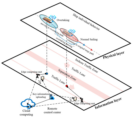
Figure 1.
Traffic separation schemes and individual vessel behavior in the waterway.
By focusing on these core behavioral types, we aim to develop a comprehensive model for understanding and predicting vessel behavior under varying maritime conditions, ultimately reducing the likelihood of collisions and improving overall safety in waterway traffic. Understanding these behavior patterns is essential for designing systems that can dynamically adjust to the constantly changing traffic environment, thus mitigating the risk of accidents and ensuring smoother, safer navigation in inland waterways.
2.2. Vessel Description and Dynamics
The motion of the vessel is modeled using a 3-DoF hydrodynamic model, as shown in Figure 2, with the kinematics and kinetics formulations represented as:
where represents the position and orientation of the vessel, is the rotation matrix, and . The variables denoted by correspond to the velocities in the surge, sway, and yaw directions. The symbol represents the inertia matrix, represents the Coriolis and the centripetal matrices, and represents the damping matrix. Furthermore, denotes the vector of control inputs.
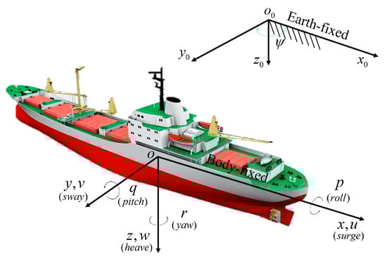
Figure 2.
Reference frame.
In the field of navigation practice, the control input often involves the manipulation of the rudder angle. Consequently, to effectively tackle the issue at hand, namely, trajectory tracking with multi-obstacle avoidance, the following transformation is implemented in a direct manner:
where represents the rudder angle, represents the propeller thrust, and , , , , , , and are model parameters. The relationship between sway velocity and rate of turn, denoted by , can be established by both full-scale and laboratory tests. The parameters , , and are associated with a simplified Nomoto model.
Let be a vector, without loss of generality. Equation (3) can be converted into the subsequent nonlinear control system.
where , , and .
If two vessels risk colliding, international or local maritime norms dictate that action must be initiated immediately. Nevertheless, establishing a secure separation distance between the two watercrafts can present a complex task. This article proposes a technique for estimating the geometry of the target vessel domain and suggests the shortest passing distance. This study employs dynamic ship domain models that consider many factors, such as navigable canal conditions, ship behaviors, ship types, and ship sizes.
Based on the above ship domain research, vessels transiting the channel must maintain a minimum safe distance from other vessels traveling in the same longitudinal direction when navigating a channel. This process establishes the vessel’s primary axis navigation domain. Furthermore, it is imperative for vessels to uphold a prescribed minimum safe distance from other vessels in adjacent lanes within a multi-lane waterway to establish the minor axis of the vessel’s domain.
Stopping visual range may be used to detect the principal axis of the vessel domain for vessels traversing the channel. In the field of traffic engineering, the concept of stopping visual range pertains to the minimum distance at which a vehicle must come to a stop when the driver hits impediments or when the preceding vehicle halts. This calculation takes into consideration factors such as response time, stopping distance, and the appropriate safe distance.
where variable represents the stopping visual range for a vessel, whereas denotes the safe distance, which is approximately equivalent to one-fourth of the vessel’s length [20]. In this context, represents the distance required for a vessel to react, denotes the distance needed for the vessel to brake if there is no vessel behind, the value of is 0, signifies the initial speed of the vessel, is the vessel operator’s response time, and is the braking rate of the vessel behind.
Suppose the channel navigation standard establishes a safe distance from vessels ahead or behind. This specified safe distance may be used as the principal axis of the vessel domain for vessels sailing along the channel. The vessel’s domain minor axis may be calculated following the Guidelines for the Design of Approach Channels, the Code for Design of General Layout of Sea Ports, the European Code for Inland Waterways, or any other applicable design guidelines for limited water channels.
The main axis is , the minor axis is , the track width is , and the safe reach width is .
3. Vessel Behavior Decision-Making System for ASV in Waterway Channels
This section presents an advanced decision-making and planning algorithm for autonomous surface vessels, designed to enhance safety and reduce accident risks in waterway navigation.
3.1. Overview of the Decision and Planning System for Vessel Behavior
Figure 3 illustrates the architecture of the proposed vessel behavior decision-making system, which integrates real-time decision-making with optimal trajectory planning. This system is essential for autonomous vessels navigating waterway channels, with a primary goal of collision avoidance and enhanced safety throughout the vessel’s journey from origin to destination. The system’s design emphasizes continuous monitoring of both the vessel’s own movement and the surrounding traffic dynamics, addressing the critical need for a robust decision-making process that adjusts to real-time conditions and minimizes the risk of accidents.
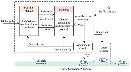
Figure 3.
Proposed decision-making and planning system architecture.
A fundamental aspect of the proposed system is the continuous safety assessment, which ensures the vessel’s behavior remains responsive to dynamic environmental factors, thereby maximizing onboard safety. At the core of this system is a conditional state machine that performs high-level decision-making, categorizing vessel behavior into three main operational states: normal sailing, overtaking, and head-on encounters. These states are designed to ensure that the vessel can safely navigate through different traffic situations, minimizing the likelihood of collision.
The decision-making process begins with an evaluation of the vessel’s current safety environment, which includes assessing the proximity and relative movement of nearby vessels. Based on this evaluation, the system then determines the appropriate collision avoidance strategy, which is implemented using chance-constrained model predictive control. MPC ensures that the vessel’s maneuvers remain both safe and efficient by predicting future states of the vessel and surrounding vessels, and then adjusting the trajectory to avoid potential collisions.
For collision avoidance scenarios, the system utilizes a chance-constrained model predictive control approach. The proposed controller optimizes the vessel’s trajectory by minimizing a cost function, while adhering to safety constraints and environmental considerations. These constraints are derived from both the vessel behavior model and real-time risk assessments, which consider the positions, velocities, and potential movements of other vessels in the waterway.
The cost function embedded in chance-constrained model predictive control evaluates various factors, such as sailing efficiency, collision risk, and maneuver feasibility, ensuring that the resulting path is not only secure but also minimizes the time spent navigating hazardous areas. The system’s design prioritizes safety by adjusting the vessel’s speed, trajectory, and behavior according to the risk levels identified during the decision-making process. This dynamic response allows the NMSV to adapt to fluctuating traffic conditions and avoid conflicts with other vessels.
3.2. Regulation-Aware Conditional State of Vessel Behavior
Traffic safety and collision avoidance are paramount in autonomous vessel navigation, especially in dynamic and congested waterways. The hierarchical conditional state machine is critical in determining the vessel’s navigation state and executing safe maneuvers, particularly under hazardous conditions. The hierarchical conditional state machine divides the vessel’s navigation behavior into two primary states: normal sailing and collision avoidance, adjusting in real time based on environmental changes and traffic conditions.
A core element of this system is the hierarchical conditional state machine model, which operates across three key decision layers: mission decision, scenario analysis, and execution action. This hierarchical approach allows for adaptive decision-making by continuously evaluating real-time traffic data, vessel status, and environmental factors. The primary objective is to reduce the risk of traffic conflicts and ensure safe navigation, aligning with the overarching goal of preventing maritime accidents and enhancing waterway safety. Each layer collaboratively processes real-time traffic data and the vessel’s status, as shown in Figure 4, ensuring informed and adaptive decision-making.
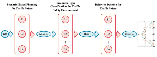
Figure 4.
Task network diagram.
3.2.1. Scenario-Based Planning for Traffic Safety
This study integrates an advanced planning model, inspired by the approach of Wang et al. [27], tailored to autonomous surface vessels navigating in narrow and busy waterways. The planner is particularly effective in structured environments, such as urban canals, where vessels face significant traffic congestion and obstacles. By ensuring robust navigation in such challenging environments, the planner contributes directly to minimizing collision risks and enhancing waterway safety.
The planning system consists of a multi-layer architecture, comprising a global planner and a local planner. The global planner utilizes vector maps to generate an initial route, maintaining a right-side alignment in the waterway to avoid collision risks with oncoming vessels and obstacles. The local planner, on the other hand, assesses real-time traffic conditions and dynamically adjusts the vessel’s trajectory by considering potential obstacles, ensuring a collision-free path while also optimizing travel efficiency.
This hierarchical planning approach shifts between four key navigational states—normal sailing, overtaking, avoidance, and lane return—depending on the environmental context and traffic conditions. By continuously updating the vessel’s behavior according to these states, the system ensures that the vessel avoids conflicts and follows the safest route to its destination. The system’s adaptability allows it to prioritize collision avoidance, making safety the primary concern, especially in critical scenarios.
The global planner optimizes route efficiency using dynamic programming and vector maps. This approach significantly reduces the risk of collision with stationary or moving obstacles while maintaining an optimal travel path. The vector map approach is designed to simplify the planning process by focusing on key waypoints and boundaries, which makes it well suited for narrow waterway navigation where avoiding obstructions is a priority.
In contrast, the local planner dynamically recalculates the best trajectory by considering real-time obstacle data. This process uses the nonlinear iterative conjugate gradient method to smooth trajectories and avoid any detected obstacles, ensuring that the vessel navigates safely and efficiently through the waterway. The local planner’s ability to adjust for obstacles in real time makes it a key element in accident prevention by minimizing the likelihood of collisions.
To evaluate potential paths, the system applies an additive cost function for each candidate trajectory, considering several factors such as deviation from the centerline, potential for collision, and overall efficiency. The cost function is defined as:
where is the th candidate trajectory’s cost function. The cost of moving away from the center point is denoted by . For each possible trajectory, there is a corresponding cost, denoted by . The cost of a collision with a static obstacle is denoted by , while the cost of a collision with a moving obstacle is denoted by . The most cost-effective candidate is selected as the optimal path without obstructions. By minimizing this cost function, the planner selects the safest and most efficient trajectory, thereby reducing the likelihood of accidents.
3.2.2. Encounter-Type Classification for Traffic Safety Enhancement
In autonomous navigation, understanding and responding to various traffic scenarios is crucial for effective collision prevention. This section focuses on classifying the type of encounters between vessels to ensure that the decision-making system can execute the appropriate collision avoidance strategy in different traffic situations. This encounter-type classification is based on a finite state machine (FSM), which helps the system adapt to changes in traffic conditions and prevent accidents by always selecting the safest behavior.
In this context, the traffic environment is categorized into normal sailing and collision avoidance states. These states are further subdivided into sub-scenarios, depending on the relative positions and velocities of other vessels in the area. The classification of these sub-scenarios is based on the Kooij model [28], which allows the system to dynamically adjust to the traffic context and execute the necessary maneuvers to prevent accidents.
The graphic above depicts the top-level state machine splitting choices in response to a typical scenario involving a vessel traveling between ports A and B.
Distance Definition for Collision Risk Assessment
One critical factor in collision avoidance is accurately assessing the potential collision risk based on the distance between the vessel and surrounding traffic. This distance, typically represented as the nearest point of approach (NPA), is calculated using curved coordinates in Cartesian space to reflect the actual waterway geometry and vessel positions. The distance function can be expressed as:
where is the projected distance for the th vessel in traffic. The Gauss–Legendre quadrature, which may be stated as follows, is used for the numerical integration to improve computation efficiency.
Here, denotes the th vessel’s weighted distance in the waterway traffic. The relative weights for the along-track and cross-track directions are denoted by and , respectively. As the vessel’s weight increases, it must avoid more available places in that direction. The symbol is used to denote the roots of the Legendre polynomial, whereas denotes the quadrature weights.
Encounter Analysis Based on Along-Track Distance
The analysis of a traffic vessel’s encounter scenario is based on the along-track distance, which represents the distance between the vessel and another vessel along the path of travel. This is crucial for assessing the relative positions of vessels in busy waterways, where accurate distance measurements are necessary to evaluate potential risks. The method for determining the along-track distance is as follows:
where is the distance along the track for the th traffic vessel. The function yields the sign of the variable provided as an argument.
To ascertain the presence of a traffic vessel, a variable is generated for the th traffic vessel, utilizing in the following manner:
The variables and are the threshold values used to make the encounter choice. By calculating the along-track distance in real time, the system can continuously monitor the traffic situation and adapt the vessel’s behavior to ensure safe separation.
Rule-Based Encounter-Type Classification for Safety
Once the relevant traffic vessels are identified, the encounter scenario must be classified according to established rules to guide the decision-making process. These rules, drawn from the International Maritime Organization (IMO) regulations, specifically the COLREGs (International Regulations for Preventing Collisions at Sea), provide a framework for safe navigation in narrow or congested waterways.
For example, rule 9 of the COLREGs requires vessels navigating narrow channels to keep as close as possible to the right-hand side of the waterway to avoid obstruction. In the case of a head-on encounter or when overtaking another vessel, the system uses these rules to classify the encounter type :
where is along-track speed. According to the International Maritime Organization (IMO), rules 9(b) and (c) establish restrictions on vessels that prevent them from obstructing the passage of another vessel that is capable of safely navigating only within a restricted channel. In situations where obstruction is unavoidable, rule 9(d) prohibits vessels from crossing the channel.
Hence, the way of categorizing encounter types based on rules considers solely head-on and overtaking scenarios, while disregarding crossing instances. These encounter classifications help determine the appropriate maneuver, such as overtaking or heading for a safer trajectory, to prevent collision risks and ensure smooth traffic flow in narrow waterways.
3.2.3. Behavior Decision for Traffic Safety
The behavior decision layer plays a crucial role in determining the autonomous vessel’s responses to varying navigational conditions, ensuring safety through effective decision-making. The system continuously monitors the surrounding environment and adjusts the vessel’s path to avoid potential collisions. When a dangerous situation arises, the vessel must execute a timely and efficient collision avoidance maneuver to ensure its safe navigation. This decision-making process is divided into three distinct phases: route evaluation, trajectory planning, and maneuver execution. Throughout each phase, the system continuously reassesses the situation, ensuring the vessel’s safety as its operational state evolves.
The hierarchical conditional state machine depicted in Figure 5 is responsible for these decision-making transitions. It generates appropriate control states based on environmental conditions, such as vessel proximity and safety distances, using mathematical constraints. The system employs a chance-constrained model predictive control (CC-MPC) algorithm to generate optimal trajectories, ensuring that safety constraints are met while minimizing the risk of accidents. The following sections provide a detailed discussion of the decision-making process, particularly focusing on how the system responds to traffic conditions, adjusts safety margins, and avoids collisions.
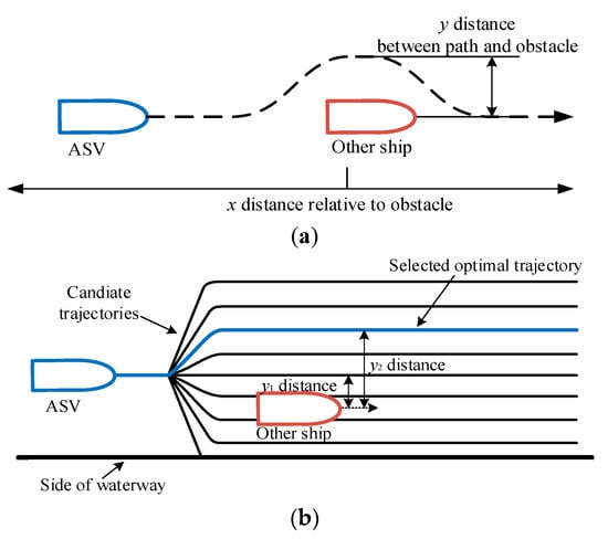
Figure 5.
Working principle of the local planner for surface vehicles. (a) Planning result; (b) planning process.
State 1: Normal Sailing
During normal sailing, the autonomous vessel maintains its course while adhering to predefined safety standards. One key aspect is the longitudinal safety distance from the vessel ahead. The vessel’s speed is adjusted to maintain this distance while tracking the preceding vessel’s trajectory. This ensures a safe buffer zone that minimizes the risk of rear-end collisions. This distance should be maintained with a consistent time gap, as depicted in Figure 6.
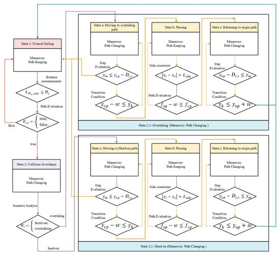
Figure 6.
Conditional state machine of sailing.
Mathematically, the required longitudinal safety distance is defined by:
The symbol represents the longitudinal safety distance for the preceding vessel, where represents the length of the vessel, represents the headway time of the preceding vessel, and represents the speed of the current autonomous vessel.
The primary objective of route maintenance is to ensure the preservation of the central location of the designated goal route. The autonomous vessel is required to maintain an appropriate longitudinal safety distance from the preceding vessel while accurately tracking the initial goal of the preceding vessel speed.
The reference values for these requirements may be observed in Figure 7 by Equation (15).
where represents the planning speed of the preceding vessel, with the symbol signifying the anticipated longitudinal state of the preceding vessel at the final step of the prediction horizon, denoted as . Additionally, the autonomous vessel must ensure the maintenance of both longitudinal and lateral safety distances (referred to as and ) simultaneously.
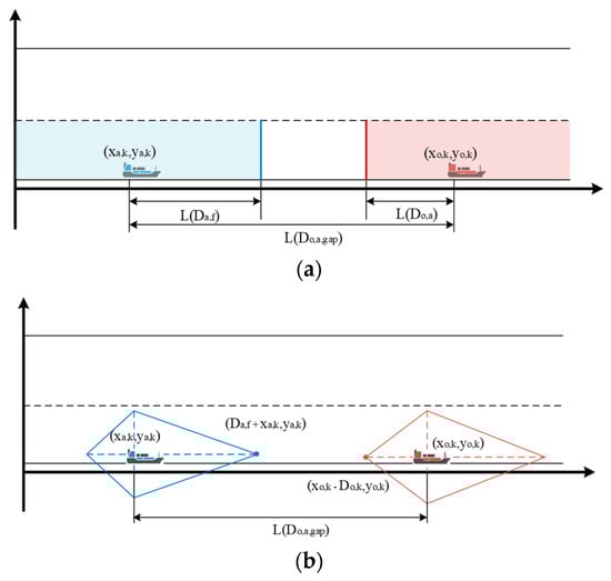
Figure 7.
Desired conditions of normal sailing. (a) Desired constraint on the horizontal axis, (b) Vessel domain.
In normal sailing practices, the process of state transition is managed by the utilization of state evaluation processes. Each step in the sample involves an evaluation of the route, with the initial goal route being referred to as the current route, and the subsequent route being referred to as the assessed route. When the evaluation cost of the subsequent route is lower than the cost of the initial target route, the status is transitioned to State 1, as depicted in Figure 7. If the cost function of the adjacent route is more favorable, it is not advisable to alter the current route of the autonomous vessel if certain requirements are met. These conditions include the obstruction of the autonomous vessel’s path and the proximity of a surrounding vessel within a specified distance . Therefore, in the present scenario described by Equation (16), the conditional state is moved to State 1.
To address the limitations associated with using only TD-error, such as the lack of diversity and the bias issue, two methods are introduced, including the stochastic sampling method and the importance sampling method. The stochastic sampling method ensures that all samples in the replay memory buffer have a non-zero probability of being sampled while guaranteeing the diversity of training data.
The constant is multiplied by the length of the vessel to obtain the side block distance.
State 2: Moving to Overtaking Path
Overtaking requires careful consideration of the relative motion between vessels. The vessel must assess multiple potential obstacles, including preceding and trailing vessels. The primary concern during overtaking is to maintain a safe distance from these vessels while preventing suction effects that could disrupt navigational stability. As seen in Figure 8, the transverse spacing between vessels should prevent suction from compromising navigational safety.
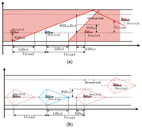
Figure 8.
Desired conditions of avoidance. (a) Desired constraint of avoidance, (b) Vessel domain.
The safety constraint for avoiding obstacles can be defined by Equation (17). These constraints are linear inequalities that are derived from the assumption of linear movement of nearby vessels and are incorporated into quadratic programming.
where represents the longitudinal safety distances between the original target preceding, adjacent preceding, and adjacent tailing vessels. The variable represents the secure lateral separation between vessels, while signifies the duration of time between the trailing vessel and the preceding vessel. The variable denotes the present velocity of the following vessel in proximity. Additionally, and represent the widths of the waterway and the vessel, respectively.
When a lane change is performed, the lateral location shifts from the lane that was initially targeted to the lane that is adjacent. The autonomous vessel is responsible for keeping enough longitudinal safety distance between itself and the vessel that is traveling in the adjacent lane. It is foolish to change lanes without first assessing the flow of traffic in the lane that will be adjacent to the one you are leaving.
where represents the lateral reference position of the last time step, and is the width of the waterway lane. As can be seen in Figure 8b, a typical traffic gap exists after the total of the preceding vessel. When changing lanes, the goal is to maintain constant awareness of the center location of the lane to which you are shifting. The autonomous vessel is responsible for monitoring the speed of the vessel in front of it and keeping the appropriate spacing between itself and the preceding vessel along both the longitudinal and the lateral axes; the reference values for a normal traffic gap are defined in Equations (18)–(20). However, when there is a high volume of traffic, there is insufficient space for a safety gap. As a result, the autonomous vessel needs to perform a nudge motion, which creates an intersection of the safety boundary. It first demonstrates the autonomous vessel’s intention to change lanes, and then it begins the process of negotiating with the adjacent tailing vessel by demonstrating its intention and observing the reaction it receives from the autonomous vessel. It is possible that this technique will increase safety by inducing a yield in the tailing vessel. This will happen throughout this operation. Because of this, engaging in this conduct is something that ensures one’s safety. The reference values for the dense gap are defined as in Equations (18)–(20), and the autonomous vessel must be situated at the cross point of the linear safety restriction for preceding and trailing vessels in the adjacent lane. When the vessel that is trailing you slows down, the distance between the two of you will grow if the trailing vessel has a cooperative inclination. After that, the self-navigating ship can switch lanes. If the vessel that is trailing you tends to be aggressive, the space will become smaller as the vessel that is trailing you increases its speed. After that, the autonomous vessel needs to head back in the direction of the primary target lane. Because the target point is in a position that is assured to be secure, it is possible to make a nudging motion that Is risk-free.
State 3: Overtaking Passing
When overtaking, the autonomous vessel must follow the preceding vessel closely while ensuring that the gap remains within the calculated safety margins. The reference values for this maneuver are derived from the current position of the preceding vessel and its relative velocity.
The safety constraints during passing are formulated as:
The neighboring lane-driving reference values are defined by Equation (22):
In the present condition, the primary lane of interest is evaluated, while the adjacent lane serves as the focal point for lane analysis. State 3 is activated when the evaluation cost of the original target lane is lower than the cost of the nearby lane.
State 4: Overtaking Passing
After successfully overtaking, the autonomous vessel must return to its original lane. This transition is managed by ensuring that the vessel maintains safe distances from both the preceding and the trailing vessels. The lateral position is adjusted, and the vessel realigns with its intended trajectory.
The constraints governing this maneuver are mathematically defined by:
where represents the longitudinal safety distance for the initial target vessel being followed. Equation (24) establishes the reference values for returning to the original goal path:
State 5: Moving to Head-on Path
When encountering an obstacle head on, the autonomous vessel must move towards a safer path, avoiding direct collisions by adjusting its heading. During this phase, the system continuously evaluates the relative positions and velocities of surrounding vessels to ensure safety.
As depicted in Figure 9, the safety constraint for obstacle avoidance can be defined by Equation (25). These constraints are linear inequalities that are derived from the assumption of linear motion of nearby vessels and are incorporated into quadratic programming.
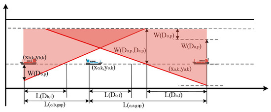
Figure 9.
Desired head-on conditions.
State 6: Head-on Passing
During head-on passing, similar to overtaking, the autonomous vessel must maintain a safe distance from both the preceding and the trailing vessels. The reference values for the maneuver ensure the vessel does not deviate from its intended path while avoiding collisions.
The lateral separation is managed by:
The neighboring lane-driving reference values are defined by Equation (27).
The reference values ensure that the autonomous vessel passes the other vessel safely without compromising the safety of surrounding traffic.
State 7: Returning to Original Target Lane After Head On
After a successful head-on avoidance maneuver, the vessel returns to its original lane. The safety constraints governing this transition are similar to those for returning after overtaking. The system ensures the vessel maintains proper safety margins while navigating back to the designated path.
The constraints for returning are mathematically expressed by:
The variable represents the longitudinal safety distance pertaining to the target vessel that is being first pursued. Equation (29) establishes the reference values for returning to the original goal path.
Once the vessel is safely aligned with its original trajectory, the system allows for the transition back to normal sailing conditions.
3.3. Chance-Constrained MPC
The architecture of optimal sailing motion planning utilizing chance-constrained model predictive control is depicted in Figure 10. The planning algorithm must conform to certain constraints to determine the safest path by utilizing the cost function, incorporating planning and control goals based on reference and weighted variables. The vessel dynamics guarantee that the produced trajectory is acceptable for vessel movement, while the physical restrictions ensure that the generated trajectory considers the actuator’s physical limitations. Constraints play a vital role in improving the trajectory’s quality by considering predefined limitations such as the maximum speed allowed by traffic rules. Furthermore, the prediction uncertainty may be addressed when the MPC is limited. The safety limits guarantee that the vessel follows a safe trajectory that avoids colliding with other vessels. The subsequent section will provide a comprehensive analysis of the specific cost functions and constraints of the model.
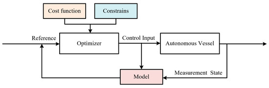
Figure 10.
Optimal planning using MPC architecture.
3.3.1. Vessel Dynamics Model
MPC’s fundamental premise is forecasting system behavior using a dynamic model, which optimizes the prediction for the optimum choice. Thus, at each time step, a prediction model is required to forecast the system’s future state given the inputs and present state.
However, the dynamics given in Section 2 are very nonlinear. The terms “predictive horizon” and “control horizon” are defined as and , respectively. The anticipated states inside the future horizon can be obtained in a sequential manner.
where is the vector of the predicted state at using the state information at . represents the control input vector. Note that . Assume that when , . This assumption is prevalent and justifiable in model predictive control applications, as it is customary to apply only the initial control action from the control sequence to the plant.
Thus, chance-constrained model predictive control solves an optimization problem to discover the actions that maximize performance across the prediction horizon at each time step.
3.3.2. Optimization Problem for Chance-Constrained Model Predictive Control
The optimal trajectory is computed at discrete time intervals T by the solution of a finite-time optimal control problem. The optimization issue represented by Equation (32) can be classified as a quadratic programming problem. The optimal value is determined through the utilization of convex optimization programming in this approach.
The equation labeled as Equation (32) represents a cost function, whereas denotes the prediction horizon step, which is specifically specified as a value of 35. The matrices and are diagonal matrices that reflect the weight factors for tracking performance in the prediction state and the final horizon step state, respectively. The variables and correspond to the costs associated with collision avoidance and grounding, respectively. The matrices and are diagonal matrices that reflect the weight factors for the tracking performance of the control input and control input rate, respectively. The symbol denotes the rate at which the control input changes.
The motion plan is technically defined as a cost function, represented by the mathematical expression in Equation (31). The prediction state is determined by the vector of reference values, whereas the final horizon step is defined according to Equation (33). These definitions are outlined in the decision-making module, which is further detailed in Section 3. Furthermore, it is imperative that the velocity, yaw rate, and yaw angle remain within reasonable limits. Subsequently, Equation (33) establishes the definition of reference values.
The following equation determines the rate of control input:
The grounding penalty is computed as follows:
where indicates the threshold of each channel’s side, serving as one approach.
This regulation pertains to the navigation of vessels inside narrow waterways, taking into consideration the adherence to right-hand traffic principles. The cost associated with adhering to rule compliance, denoted as , is determined by evaluating the cross-track locations required to conform to right-hand traffic regulations, as illustrated below:
The estimation of collision cost can be determined by calculating the closest pairwise distance between the path and traffic vessels at each point along the channel.
where is the conflict radius used to smooth out the cost’s discontinuity [29]. Figure 11 displays the expenses associated with adhering to regulations (represented by the orange line) and the costs of grounding (shown by the blue line) within the vertical segment of the channel. The collision cost is estimated in our framework using a function that quantifies the risk of collision between the autonomous vessel and nearby ground. The approach used to estimate the collision cost and the function is based on methods that have been widely used in maritime navigation and collision avoidance systems. Specifically, Cho et al. [30] introduced a similar approach for COLREG-compliant ship collision avoidance in narrow channels using curvilinear coordinates. Their method also emphasizes the importance of functions for collision risk estimation in dynamic environments.
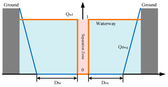
Figure 11.
The cost is associated with adhering to regulations and the act of temporarily immobilizing a vessel in the vertical portion of a waterway. The cross-track position is represented by the horizontal axis, while the vertical axis represents cost. The yellow areas depicted in the diagram correspond to the terrestrial areas located on each side of the waterway.
3.3.3. Constraints for Chance-Constrained Model Predictive Control
To ensure safe and efficient vessel operation in dynamic maritime environments, it is essential to account for the physical limitations of the vessel’s actuators and the inherent uncertainty in surrounding traffic conditions. The control input and its rate are constrained to avoid overloading the vessel’s actuators. These constraints are mathematically represented as follows:
where and represent the upper and lower bounds of the control input. Additionally, let and represent the upper and lower limits on the rate of change of the control input, respectively.
In addition to the actuator constraints, the trajectory planner must also account for maritime traffic regulations and vessel speed restrictions. The maximum speed restriction of the vessel, denoted as , is crucial for maintaining safe operation, particularly when navigating congested or high-traffic areas. The speed limitations and the corresponding trajectory adjustment are governed by:
A key challenge in this dynamic environment is the uncertainty in predicting the behavior of surrounding vessels. This uncertainty introduces noise into the motion planning process, which can lead to suboptimal or unsafe trajectory choices. To address this issue, the chance constraint is incorporated into the model predictive control (MPC) framework. This constraint ensures that the vessel remains within a probabilistic safety envelope, thereby enhancing the robustness of the decision-making process under uncertain conditions. The chance constraint is formulated as:
where is the chance constraint parameter and is the autonomous vessel state, and is surrounding vessel state safety constraint matrixes. Section 3.3 details the design of these limitations. However, due to its stochastic nature, this constraint cannot be applied in convex optimization. Its computation is depicted in Equation (41).
where denotes the covariance of the Gaussian distribution of the process noise.
The parameter for the chance constraint is proportional to the prediction uncertainty. This adjustable parameter controls the planning algorithm’s properties. For example, if is a huge value, the algorithm creates a route that prioritizes travel efficiency. On the one hand, when the value of is minimal, the method produces a result that enhances safety by including the uncertainty linked to the forecast of the environment.
By incorporating these constraints into the trajectory planning process, the autonomous vessel can make informed decisions that balance operational efficiency with the imperative of minimizing collision risks. This method aligns with the goal of improving maritime safety, particularly in high-traffic environments, where decision-making precision is essential to avoiding accidents and enhancing navigational safety.
4. Case Study
4.1. Experimental Settings
This section presents the evaluation of the proposed autonomous vessel navigation and collision avoidance system, with a focus on preventing traffic accidents and enhancing navigational safety in maritime environments. Three distinct scenarios are examined: the first test demonstrates the robustness and real-world applicability of the system on an actual USV, as shown in Figure 12, the second examines the path planning and avoidance performance in head-on and overtaking situations, and the third evaluates the vessel’s ability to navigate safely in a complex, dynamic waterway environment. These case studies aim to assess how the proposed framework can effectively reduce traffic conflicts and improve safety by preventing accidents through proactive decision-making and optimized path planning.
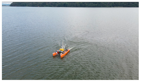
Figure 12.
The unmanned surface vessel used in the tests.
To ensure replicability, the experiments were conducted using publicly available software (MATLAB2023a and FORCES PRO 4.2). The experiments can be replicated by adjusting the key parameters, such as the control horizon Hp, the number of vessels, and the density of obstacles. The model was tested for various traffic densities, ranging from sparse to congested conditions. The hardware configuration for these simulations includes an Intel i7-12700 CPU, an Nvidia GeForce RTX A2000 8 GB GPU, and 32 GB of RAM, ensuring efficient and reliable computational performance.
The non-convex model predictive control MPC problem, as defined in Equation (32), is solved using a 7 s planning horizon and 35 planning steps, with optimization performed through the FORCES PRO tools. This methodology enables effective management of complex, real-time maritime scenarios, ensuring that the vessel’s decision-making and trajectory planning are optimized for both safety and operational efficiency. The model parameters are given as , b = 0.62, , , , , , and . The propeller thrust is constrained in .
4.2. Real-World Experimental Study
To assess the performance of the proposed system in real-world conditions, a simulated waterway channel was created with a width of 200 m and a length of 900 m, representing a typical narrow and congested waterway. The goal of the experiment was to demonstrate how the proposed system could mitigate the risks associated with traffic conflicts and improve safety, especially under challenging environmental conditions, such as wind, waves, and sensor uncertainty.
The experimental environment includes three static obstacles placed within the waterway channel: two circular obstacles and one rectangular obstacle. These obstacles were simulated as virtual physical entities, representing common hazards that could impede the safe navigation of vessels in busy waterways. The radius of the first circular obstacle is set to 26 m, the second is set to 13 m, and the rectangular obstacle measures 95 m in length and 21 m in width. These obstacles serve as realistic representations of the types of hazards that could lead to traffic conflicts or accidents in congested waterway environments.
The real-world experiment evaluates the vessel’s ability to navigate through the waterway channel at a target speed of 4 m/s while avoiding static obstacles. The vessel autonomously adjusts its path in real time to avoid collisions, as shown in Figure 13. The key events are as follows:
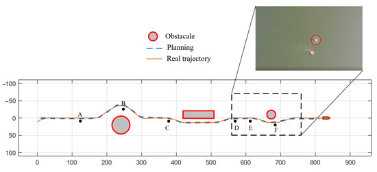
Figure 13.
The performance of the vessel’s sailing with static obstacles (Scenario 1).
At Time A, the vessel detects the first obstacle in its path.
At Time B, the vessel alters its course to avoid the obstruction.
At Time C, a similar maneuver is performed to circumvent a second static obstacle.
At Time D, the vessel continues its original trajectory, preparing for the next obstacle.
At Time E, the vessel detects another obstruction and evaluates its safety margin.
At Time F, the vessel adjusts its course to avoid the newly identified hazard and continues toward its destination.
Throughout the test, the vessel successfully avoids all obstacles, demonstrating the system’s capability to prevent accidents by maintaining a safe distance from potential collisions. The ability to adapt to dynamic obstacles in real time underscores the effectiveness of the decision-making and planning algorithms in preventing traffic conflicts and ensuring safe navigation.
Figure 14 presents the surge velocity and yaw rate results for the vessel in Scenario 1. These measurements show how the vessel adjusts its speed and heading to maintain a safe path while avoiding obstacles. The real-time adjustments are critical for preventing accidents, as the vessel is able to respond dynamically to the detected obstacles and avoid unsafe trajectories. These data further confirm the ability of the proposed system to not only navigate safely but also optimize efficiency, a key factor in accident prevention.
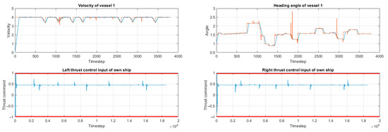
Figure 14.
Surge velocity and yaw rate results of the vessel in Scenario 1 (red dashed line is the statement’s boundary, orange line is ref velocity and heading angle of vessel and blue line represents the true value of the corresponding variable).
4.3. Simulation Evaluation in Typical Scenarios
Simulation case study 1 simulates a dynamic maritime environment featuring four moving vessels. The scenario includes two overtaking situations and one head-on encounter, all of which adhere to maritime traffic regulations. These simulated conditions are crucial for testing the effectiveness of our proposed collision avoidance strategies and their ability to enhance navigational safety.
Simulation case study 2 simulates a more complex waterway scenario involving four vessels, with their initial positions randomly generated within a predefined area of an inland traffic separation scheme at Rotterdam Port. This simulation helps evaluate the system’s ability to manage multiple vessels navigating simultaneously, ensuring safe interactions and minimizing collision risks in busy waterway environments.
- (1)
- Case study 1: Sailing in a dynamic vessel environment
In this case study, we simulate an overtaking scenario involving several vessels navigating through an inland waterway. The presence of multiple moving vessels introduces unpredictability, allowing us to assess the resilience of our decision-making model in real time. The simulation also includes vessels that deviate from established navigation laws to test the algorithm’s robustness under more chaotic conditions.
Figure 15 illustrates a comprehensive traffic scenario comprising three consecutive sub-scenes, showcasing how the research vessel interacts dynamically with surrounding vessels. In this simulation, one of the vessels in the scenario violates maritime navigation regulations, introducing unpredictability into the system, which is designed to test how well the decision-making model handles more complex, less predictable traffic conditions. This approach simulates a more realistic environment, allowing the decision model to better manage unpredictable vessel movements and enhance its collision prevention capability.
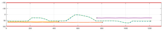
Figure 15.
The performance of multi-vessel sailing in the waterway (Scenario 1, the lines of different colors represent the navigation trajectories of different ships).
The proposed chance-constrained model predictive control controller governs the movement of the vessels in the simulation. While the environmental vessels follow a straight path, the autonomous vessel adjusts its trajectory based on surrounding dynamic changes. This ability to react to real-time environmental shifts is crucial for mitigating potential traffic conflicts and improving safety in busy waterway environments.
The simulation reveals that the autonomous vessel adheres to prescribed reference paths but adapts when it encounters the boundary conditions for state switching. At this point, the state machine evaluates multiple states and dynamically adjusts the predictive control constraints to prevent accidents, rerouting the vessel to avoid collision risks and navigating safely.
Figure 16 illustrates the simulation of an overtaking maneuver. Initially, the orange vessel is overtaking a slower-moving blue vessel. The safety gap is maintained, ensuring no collisions occur during the overtaking process. As shown in Figure 16b, the autonomous vessel adjusts its path in real time to safely overtake, while the red line marks the safety limit. The vessel initiates a nudge maneuver (Figure 16d) and successfully moves into the opposite lane to complete the overtaking action. After the maneuver, the vessel returns to its designated path, as shown in Figure 16e.
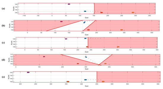
Figure 16.
Overtaking process in the case study of Scenario 1 (the red dashed line is the planning boundary), (a–e) displays the traffic status of ships at different times during the overtaking process, the polygons of different colors in the figure represent the corresponding ships.
During the simulation, velocity and angular velocity data (Figure 17a) show that the autonomous vessel increases speed to overtake the slower vessel, then returns to its original trajectory at the optimal speed for efficient navigation. Safety considerations are prioritized throughout, ensuring that energy consumption is minimized without compromising collision avoidance.
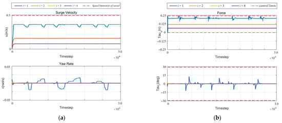
Figure 17.
Simulation results of vessels in Scenario 1. (a) Surge velocity and yaw rate results of vessel in Scenario 2 (the red dashed line is the statement’s boundary); (b) force of vessel in Scenario 2 (the red dashed line is the physical boundary).
Figure 17b depicts the forces acting on the vessel during the overtaking process. The results indicate that while energy is expended during lane changes, the maneuver is completed successfully with minimal vibrations and disruptions to the vessel’s stability.
- (2)
- Case study 2: Sailing in a waterway environment
This case study addresses the challenges of navigating multiple vessels in an inner canal system, simulating a complex scenario involving unpredictable movements and diverse traffic patterns. The primary objective is to evaluate the effectiveness of the chance-constrained model predictive control controller in ensuring safe vessel separation and preventing collisions within confined waterway spaces. By considering dynamic environmental factors, we aim to improve waterway safety through proactive collision avoidance and safe navigation strategies.
Figure 18 depicts the trajectories of four vessels in an overtaking situation. All vessels are programmed to follow the designated navigation paths, but when one vessel reaches the boundary conditions of the state-switching mechanism, the system adapts by adjusting the model predictive control (MPC) restrictions. The state machine dynamically evaluates the vessel’s position and environmental context, adjusting the control strategy accordingly to ensure safe maneuvering. As a result, the autonomous vessel adjusts its path to mitigate collision risks and avert mishaps in real time.
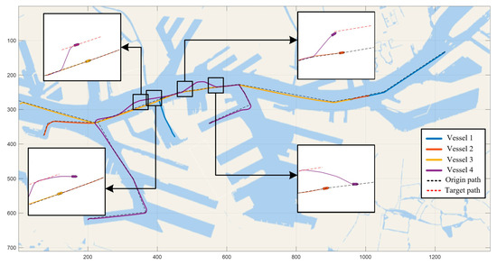
Figure 18.
The performance of multi-vessel sailing in the complex waterway (Scenario 3). The black dashed line is the initial planned path; the red dashed line is the reference path for re-planning during the collision avoidance phase.
Figure 19 shows the behavior of the vessels during normal sailing. The error in the vessel’s position and heading, controlled by the hierarchical conditional state machine and chance-constrained model predictive control algorithms, approaches zero, indicating that the vessel maintains a high degree of precision and stability in its navigation. This ensures that the autonomous vessel stays within the designated route while adjusting to the surrounding vessels and environmental conditions. The control system’s ability to minimize navigation errors is vital for collision prevention, particularly in high-density traffic scenarios.
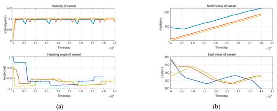
Figure 19.
Simulation results of vessels in scenario 3. (a) Position results of vessels 1, 2, and 3 (b); surge velocity and heading results of vessels 1, 2, and 3. Blue line represents Ship 1, orange line represents Ship 2, and yellow line represents Ship 3.
Despite the successful overtaking, minor oscillations in the vessel’s velocity and heading are observed. These oscillations occur due to the need for the vessel to expend energy when transitioning to the adjacent lane, which is typically denser with traffic and requires a wider time gap for a safe maneuver. This highlights the inherent trade-off between safety and energy efficiency, which must be carefully balanced in real-time decision-making to ensure safe navigation while minimizing unnecessary energy consumption.
Safety considerations play a critical role in this scenario, as the vessel adjusts its trajectory to avoid collision with the preceding vessel, demonstrating the algorithm’s ability to adapt to changing traffic conditions and ensure safe vessel operations in confined and high-risk environments.
Figure 20 illustrates the position, velocity, and heading of Vessel 4 during the overtaking maneuver. In this scenario, the autonomous vessel encounters a slower-moving vessel and, to avoid potential collision, navigates to an adjacent canal to safely overtake. After the maneuver, the autonomous vessel returns to its original course while maintaining an optimal speed, demonstrating the system’s capacity to make timely overtaking decisions.
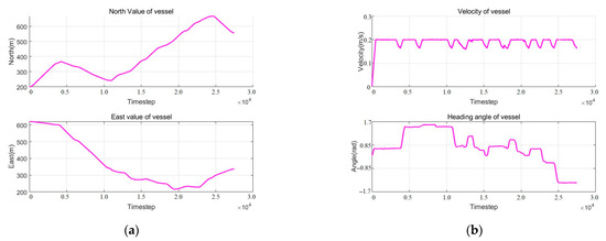
Figure 20.
Simulation results of the vessel in Scenario 3. (a) Position results of Vessel 4 (b); surge velocity and heading results of Vessel 4.
- (3)
- Comparative Analysis: Methodologies and Baseline Approaches
To further evaluate the effectiveness of our proposed hierarchical conditional state machine and chance-constrained model predictive control methodologies, we compare their performance against two baseline methods: RA-MPCC [30] and Breadth First Search (BFS) local planner with NMPC [21]. The results, summarized in Table 2, demonstrate that our approach outperforms the baseline methods in terms of collision frequency and navigation safety.
Table 2.
Results for three different random scenarios, each run twenty times. These test cases include head-on and overtaking. Out of all violations (Inland Waterway Regulations), the percentage is calculated for each run. The percentage shows the mean overall runs.
The use of hierarchical conditional state machine and chance-constrained model predictive control enables vessels to anticipate potential collisions and adjust their trajectories proactively. This allows for the initiation of avoidance maneuvers at an earlier stage, particularly in head-on encounters or overtaking situations, leading to safer navigation in congested waterways. In contrast, the BFS-NMPC approach tends to adhere too rigidly to the initial trajectory, failing to account for future obstacles, and as a result, it experiences a higher frequency of collisions and does not fully comply with inland waterway regulations.
4.4. Computational Complexity and Real-Time Performance
4.4.1. Theoretical Complexity
The worst-case complexity of the proposed framework is governed by the SQP iterations and multistage QP structure O(K⋅Hp⋅(nx + nu)3), where K = 10 (average iterations), Hp = 35, nx = 5, and nu = 2. Total FLOPs = 10⋅35⋅(5 + 2)3 = 120,050 FLOPs.
4.4.2. Measured Computation Time
Table 3 summarizes the actual computation time across three scenarios, and the results are shown in the table.
Table 3.
Computation times across three different scenarios.
Even in the worst case (Hp = 35), the maximum solve time (14.5 ms) is 85.5% faster than the 100 ms control cycle, leaving ample margin for sensor data processing and actuator communication. GPU acceleration reduces computation time by 22% compared to CPU-only execution (tested via solver profiling).
The RTX A2000 GPU significantly accelerates dense linear algebra operations in FORCES PRO. GPU-accelerated LU decomposition reduces per-iteration time by 35%. Collision avoidance constraints (Equations (37) and (38)) were batched and evaluated on the GPU, achieving a 1.8× speedup over CPU.
4.4.3. Comparison with Baseline Solvers
A comparative analysis with general-purpose solvers highlights FORCES PRO’s efficiency, and the results are shown in Table 4.
Table 4.
Comparison with baseline solvers.
FORCES PRO’s structure exploitation and GPU acceleration enable 5.8× faster solves than IPOPT. The proposed framework achieves real-time trajectory planning (5–20 ms per solve) on commercially available hardware (Intel i7-12700 + RTX A2000). By leveraging FORCES PRO’s code generation, multicore CPU/GPU parallelism, and sparsity exploitation, the method scales efficiently to complex maritime scenarios with dynamic obstacles and stochastic uncertainties. These results confirm that the computational complexity is fully compatible with real-world deployment, even under resource constraints.
4.5. Robustness Analysis
In this section, we present the results of the sensitivity analysis conducted to evaluate the impact of key parameters on the performance of the proposed decision-making framework. Sensitivity analysis helps in understanding how variations in system parameters affect the overall performance, and it allows for assessing the robustness of the system to different conditions.
The control horizon refers to the number of steps over which the model predictive control (MPC) makes predictions for the system’s behavior.
We varied the control horizon Hp to assess its effect on both computational performance and safety. A longer horizon increases the accuracy of predictions but also increases the computational complexity, as the number of optimization variables grows.
With a shorter horizon (Hp = 20), the optimization problem becomes less complex, leading to faster computation times. However, it sometimes results in reduced safety margins, particularly in dynamic environments where unexpected changes can occur.
A longer horizon (Hp = 35 H) improves the accuracy of predictions and ensures better safety, but it also increases the computational load. The system was able to maintain real-time feasibility with a horizon of 35 steps, although the average computation time increased slightly.
The system shows robust performance across a range of horizons, ensuring safety without compromising real-time feasibility, especially with the use of GPU acceleration.
4.6. Discussion
In the first real-world experiment, we evaluated the system’s performance in a simulated waterway channel with three static obstacles (two circular and one rectangular). The system demonstrated effective real-time obstacle avoidance, adapting the vessel’s path and maintaining safe distances. The autonomous vessel navigated at 4 m/s, dynamically adjusting its course to avoid obstacles. These maneuvers highlight the system’s ability to respond to environmental changes, minimizing collision risk and optimizing efficiency. However, the study did not address dynamic factors such as moving vessels or fluctuating environmental conditions (e.g., wind and waves), which require further refinement in the control algorithms to enhance performance in more variable scenarios.
In the second case study, we simulated overtaking scenarios in a multi-vessel environment to test the robustness of the chance-constrained model predictive control (CC-MPC). The system successfully adjusted its trajectory for overtaking slower vessels, maintaining safety distances and ensuring compliance with regulations. Real-time adjustments, as indicated by velocity and angular velocity measurements, balanced speed with safety during overtaking. However, unpredictable movements of other vessels, especially those violating maritime regulations, posed challenges. The system must improve its ability to anticipate complex interactions and quickly adjust to sudden changes in vessel speed.
The third case study simulated a multi-vessel scenario in a confined waterway. The CC-MPC effectively managed vessel movements by adjusting the path to avoid collisions, ensuring safe maneuvering in high-density traffic. This was especially critical when environmental constraints necessitated path adjustments. The system maintained high precision in navigation, minimizing errors in position and heading. However, oscillations in velocity and heading during maneuvers suggest a trade-off between safety and energy efficiency, highlighting the need for optimization.
A comparative analysis showed that the proposed HCSM and CC-MPC method significantly outperformed baseline methods in collision avoidance and regulatory compliance. The system demonstrated superior computational efficiency and real-time decision-making capabilities, outperforming traditional solvers such as IPOPT and fmincon, which struggled with real-time feasibility due to their higher computational demands.
In the future, the integration of Internet of Ships (IoS) will enhance the system by enabling real-time communication and data exchange between vessels and shore systems, facilitating dynamic decision-making and improving system reliability. These technologies ensure that the system can adapt to real-time traffic changes and environmental disturbances, which are critical in busy waterways where vessel behavior and environmental factors are constantly changing.
While the experiments conducted in this study focused on a specific waterway configuration and obstacle layout, the proposed framework is designed with flexibility and adaptability in mind, making it applicable to a broad range of maritime environments. The ability to dynamically adjust vessel trajectories based on traffic conditions and environmental factors ensures that the system is not confined to a single type of waterway or scenario.
The core principles of the HCSM and CC-MPC method can be easily adapted to various waterway types, including narrow channels, wide channels, rivers, and open seas. In narrow channels, where space is limited and the risk of collisions is higher, the system can prioritize safety by increasing safety margins and adopting more conservative maneuvers. For wider water bodies or open seas, where vessel interactions are less frequent, the framework can optimize vessel speeds and trajectories for greater efficiency while maintaining safe distances.
In conclusion, the generalizability of the proposed framework extends far beyond the specific waterway configuration tested in this study. Its flexibility allows it to be applied to a diverse set of maritime scenarios, ensuring that it can be effectively deployed in different waterway types, traffic densities and regulatory contexts. Future work will focus on further enhancing its adaptability and extending its applicability to even more complex real-world maritime environments.
4.7. Limitations of the Study
Despite the promising results, this study has several limitations. First, the experimental evaluations were conducted in simulated environments under controlled conditions, which did not fully capture dynamic factors such as moving vessels, fluctuating environmental conditions (e.g., wind and waves), sensor noise, and model inaccuracies. The limited obstacle configuration and specific waterway scenarios may restrict the generalizability of the findings to more diverse maritime settings. Furthermore, the observed oscillations in velocity and heading during high-density traffic indicate a trade-off between safety and energy efficiency that warrants further optimization. Future research should focus on integrating robust optimization techniques, incorporating additional dynamic environmental factors, and validating the framework under a broader range of realistic conditions.
5. Conclusions
This study investigates the application of hierarchical conditional state machine and chance-constrained model predictive control algorithms for enhancing the safety of autonomous vessels in dynamic waterway environments. The construction of the hierarchical system involves the utilization of both a hierarchical conditional state machine and a chance-constrained model predictive control technique. The implementation of a hierarchical design in this context serves to guarantee both the safety and efficiency of sailing operations, considering the necessary compliance with avoidance restrictions pertaining to the waterway as well as the prevailing environmental circumstances. The hierarchical conditional state machine establishes appropriate reference and safety thresholds for navigation by employing avoidance sub-maneuvers and adhering to the appropriate transition condition. Given the presence of forecast uncertainty, the chance-constrained model predictive controller offers an optimal, effective, and secure trajectory. The sailing propensity in the hierarchical conditional state machine stage can be altered by adjusting the weighting parameter, whereas in the chance-constrained model predictive control stage, it can be influenced by manipulating the chance constraint parameter. The experimental results demonstrate that these algorithms can effectively mitigate traffic conflicts and reduce the risk of collisions, particularly in congested and high-risk waterway conditions. By incorporating real-time decision-making and trajectory planning, the system proactively avoids accidents and optimizes vessel navigation, thereby contributing to traffic accident prevention.
The experimental results clearly indicate that the proposed framework achieves enhanced computational efficiency and safety performance under dynamic and high-density traffic conditions. However, the current framework does not fully account for uncertainties such as sensor noise, model inaccuracies, and unexpected vessel maneuvers, which are critical in real-world applications. Moreover, the experimental validation was performed within a specific simulation environment, limiting the generalizability of the findings. In future research, we plan to extend our model by incorporating robust optimization techniques to explicitly handle these uncertainties, validating the framework under more diverse and realistic scenarios, and exploring strategies to further improve energy efficiency.
Looking forward, the integration of environmental factors into the decision-making process, coupled with the optimization of energy usage, will enhance the system’s robustness. Additionally, improving real-time adaptability in complex, unpredictable traffic situations will be critical in ensuring that autonomous vessels can navigate safely in real-world conditions. Overall, we believe that these enhancements will pave the way for more adaptive and resilient autonomous maritime navigation systems, ultimately contributing to safer and more efficient waterway operations.
Author Contributions
W.T.: Literature search, figures, study design, data collection, data analysis, data interpretation, writing. L.W.: Literature search, study design, data collection, data analysis, writing. J.T.: Study design, writing, supervision. M.Z.: Writing, review and editing, supervision. Y.W.: Review and editing, supervision, project administration. All authors have read and agreed to the published version of the manuscript.
Funding
This work is supported by the H2020 Program NOVIMOVE: “Novel inland waterway transport concepts,” the National Key Research and Development Program of China through grant No. 2021YFC3101800, the National Natural Science Foundation of China (No. U2141234), the Young Talents Project of the Science Research Program of Hubei Provincial Department of Education through grant No. 2023Q20231606, Natural Science Foundation of Hainan Province of China through Grant No. 624MS079, Natural Science Foundation of Wuhan City of Hubei Province of China through Grant No. 2024040801020260, Young Elite Scientists Sponsorship Program by China Association for Science and Technology (CAST) through Grant No. YESS20230384.
Institutional Review Board Statement
Not applicable.
Informed Consent Statement
Not applicable.
Data Availability Statement
Data are contained within the article.
Conflicts of Interest
The authors declare that they have no known competing financial interests or personal relationships that could have appeared to influence the work reported in this paper.
Nomenclature
| Symbol | Definition/Description |
| navigation status of vessel at time | |
| v | vessel velocity |
| c | heading angel |
| d | vessel decision state |
| τ | vessel control input |
| position and orientation of vessel | |
| rotation matrix | |
| velocities in the surge, sway, and yaw directions | |
| inertia matrix | |
| Coriolis and centripetal matrices | |
| damping matrix | |
| stopping visual range for a vessel | |
| the ith candidate trajectory’s cost function | |
| projected distance for the ith vessel in traffic | |
| the ith vessel’s weighted distance in the waterway traffic | |
| distance along the track for the ith traffic vessel | |
| values used to make the encounter choice | |
| encounter type | |
| longitudinal safety distances between the original target preceding, adjacent preceding, and adjacent tailing vessels | |
| lateral safety distances between the original target preceding, adjacent preceding, and adjacent tailing vessels | |
| planning speed of the preceding vessel | |
| anticipated longitudinal state of the preceding vessel at the final step of the prediction horizon | |
| duration of time between the trailing vessel and the preceding vessel | |
| present velocity of the following vessel in proximity. |
References
- Wiegmans, B.; Konings, R. Inland Waterway Transport: Challenges and Prospects; Routledge: Abingdon, UK, 2016. [Google Scholar]
- Harada, H. Fundamental Field Experiments of OFDMA Systems Using VHF-band in Urban Area. In Proceedings of the 2023 26th International Symposium on Wireless Personal Multimedia Communications (WPMC), Tampa, FL, USA, 19–22 November 2023; IEEE: Piscataway, NJ, USA, 2023; pp. 154–158. [Google Scholar]
- Öztürk, Ü.; Boz, H.A.; Balcisoy, S. Visual analytic based ship collision probability modeling for ship navigation safety. Expert Syst. Appl. 2021, 175, 114755. [Google Scholar] [CrossRef]
- Tao, W.; Zhu, M.; Chen, S.; Cheng, X.; Wen, Y.; Zhang, W.; Negenborn, R.R.; Pang, Y. Coordination and Optimization Control Framework for Vessels Platooning in Inland Waterborne Transportation System. IEEE Trans. Intell. Transp. Syst. 2023, 24, 15667–15686. [Google Scholar] [CrossRef]
- Negenborn, R.R.; Goerlandt, F.; Johansen, T.A.; Slaets, P.; Banda, O.A.V.; Vanelslander, T.; Ventikos, N.P. Autonomous ships are on the horizon: Here’s what we need to know. Nature 2023, 615, 30–33. [Google Scholar] [CrossRef] [PubMed]
- Maidana, R.G.; Kristensen, S.D.; Utne, I.B.; Sørensen, A.J. Risk-based path planning for preventing collisions and groundings of maritime autonomous surface ships. Ocean Eng. 2023, 290, 116417. [Google Scholar] [CrossRef]
- Kim, J.; Lee, C.; Chung, D.; Cho, Y.; Kim, J.; Jang, W.; Park, S. Field experiment of autonomous ship navigation in canal and surrounding nearshore environments. J. Field Robot. 2024, 41, 470–489. [Google Scholar] [CrossRef]
- Cho, Y.; Park, J.; Kim, J.; Kim, J. Autonomous Ship Collision Avoidance in Restricted Waterways Considering Maritime Navigation Rules. IEEE J. Ocean. Eng. 2023, 48, 1009–1018. [Google Scholar] [CrossRef]
- Wang, C.; Zhang, X.; Gao, H.; Bashir, M.; Li, H.; Yang, Z. COLERGs-constrained safe reinforcement learning for realising MASS’s risk-informed collision avoidance decision making. Knowl.-Based Syst. 2024, 300, 112205. [Google Scholar] [CrossRef]
- Veitch, E.; Alsos, O.A. A systematic review of human-AI interaction in autonomous ship systems. Saf. Sci. 2022, 152, 105778. [Google Scholar] [CrossRef]
- Kim, J.H.; Kim, J.H.; You, Y.J.; Do Chi, S. Simulation-based effectiveness analysis of mission planning for autonomous unmanned surface vehicles (usvs). Int. J. Eng. Res. Technol. 2018, 11, 715.e24. [Google Scholar]
- Ferris, D.L.; Subramani, D.N.; Kulkarni, C.S.; Haley, P.J.; Lermusiaux, P.F. Time-optimal multi-waypoint mission planning in dynamic environments. In Proceedings of the OCEANS 2018 MTS/IEEE Charleston, Charleston, SC, USA, 22–25 October 2018; IEEE: Piscataway, NJ, USA, 2018; pp. 1–8. [Google Scholar]
- Wen, Y.; Tao, W.; Sui, Z.; Piera, M.A.; Song, R. Dynamic model-based method for the analysis of ship behavior in marine traffic situation. Ocean Eng. 2022, 257, 111578. [Google Scholar] [CrossRef]
- Murray, B.; Perera, L.P. Ship behavior prediction via trajectory extraction-based clustering for maritime situation awareness. J. Ocean Eng. Sci. 2022, 7, 1–13. [Google Scholar] [CrossRef]
- Rijksoverheid. Binnenvaartpolitiereglement. 2017. Available online: https://wetten.overheid.nl/BWBR0003628/2017-01-01 (accessed on 5 February 2025).
- Zhao, L.; Roh, M.I. Colregs-compliant multiship collision avoidance based on deep reinforcement learning. Ocean Eng. 2019, 191, 106436. [Google Scholar] [CrossRef]
- Xie, S.; Hu, J.; Bhowmick, P.; Ding, Z.; Arvin, F. Distributed motion planning for safe autonomous vehicle overtaking via artificial potential field. IEEE Trans. Intell. Transp. Syst. 2022, 23, 21531–21547. [Google Scholar] [CrossRef]
- Guo, Y.; Guo, Z.; Wang, Y.; Yao, D.; Li, B.; Li, L. A survey of trajectory planning methods for autonomous driving—Part I: Unstructured scenarios. IEEE Trans. Intell. Veh. 2023. [Google Scholar] [CrossRef]
- Turnwald, A.; Wollherr, D. Human-like motion planning based on game theoretic decision making. Int. J. Soc. Robot. 2019, 11, 151–170. [Google Scholar] [CrossRef]
- Liu, J.; Zhou, F.; Li, Z.; Wang, M.; Liu, R.W. Dynamic ship domain models for capacity analysis of restricted water channels. J. Navig. 2016, 69, 481–503. [Google Scholar] [CrossRef]
- Wang, W.; Gheneti, B.; Mateos, L.A.; Duarte, F.; Ratti, C.; Rus, D. Roboat: An autonomous surface vehicle for urban waterways. In Proceedings of the 2019 IEEE/RSJ International Conference on Intelligent Robots and Systems (IROS), Macau, China, 3–8 November 2019; IEEE: Piscataway, NJ, USA, 2019; pp. 6340–6347. [Google Scholar]
- Cho, Y.; Kim, J.; Kim, J. Colreg-compliant ship collision avoidance in narrow channels using curvilinear coordinates. IFAC-Pap. 2021, 54, 24–29. [Google Scholar] [CrossRef]
- Statheros, T.; Howells, G.; Maier, K.M. Autonomous ship collision avoidance navigation concepts, technologies and techniques. J. Navig. 2008, 61, 129–142. [Google Scholar] [CrossRef]
- Munim, Z.H. Autonomous ships: A review, innovative applications and future maritime business models. Supply Chain Forum Int. J. 2019, 20, 266–279. [Google Scholar] [CrossRef]
- Ziajka-Poznańska, E.; Montewka, J. Costs and benefits of autonomous shipping—A literature review. Appl. Sci. 2021, 11, 4553. [Google Scholar] [CrossRef]
- Chen, H.; Wen, Y.; Huang, Y.; Xiao, C.; Sui, Z. Edge Computing Enabling Internet of Ships: A Survey on Architectures, Emerging Applications, and Challenges. IEEE Internet Things J. 2024, 12, 1509–1528. [Google Scholar] [CrossRef]
- Wang, W.; Shan, T.; Leoni, P.; Fernández-Gutiérrez, D.; Meyers, D.; Ratti, C.; Rus, D. Roboat ii: A novel autonomous surface vessel for urban environments. In Proceedings of the 2020 IEEE/RSJ International Conference on Intelligent Robots and Systems (IROS), Las Vegas, NV, USA, 24 October 2020–24 January 2021; IEEE: Piscataway, NJ, USA, 2020; pp. 1740–1747. [Google Scholar]
- Kooij, C. Towards Unmanned Cargo Ships: A Task Based Design Process to Identify Economically Viable Low and Unmanned Ship Concepts; Gildeprint: Enschede, The Nederlands, 2021. [Google Scholar]
- Woerner, K.; Benjamin, M.R.; Novitzky, M.; Leonard, J.J. Quantifying protocol evaluation for autonomous collision avoidance. Auton. Robot. 2019, 43, 967–991. [Google Scholar] [CrossRef]
- De Vries, J.; Trevisan, E.; van der Toorn, J.; Das, T.; Brito, B.; Alonso-Mora, J. Regulations aware motion planning for autonomous surface vessels in urban canals. In Proceedings of the 2022 International Conference on Robotics and Automation (ICRA), Philadelphia, PA, USA, 23–27 May 2022; pp. 3291–3297. [Google Scholar]
Disclaimer/Publisher’s Note: The statements, opinions and data contained in all publications are solely those of the individual author(s) and contributor(s) and not of MDPI and/or the editor(s). MDPI and/or the editor(s) disclaim responsibility for any injury to people or property resulting from any ideas, methods, instructions or products referred to in the content. |
© 2025 by the authors. Licensee MDPI, Basel, Switzerland. This article is an open access article distributed under the terms and conditions of the Creative Commons Attribution (CC BY) license (https://creativecommons.org/licenses/by/4.0/).