Fluid–Structure Interaction of a Darrieus-Type Hydrokinetic Turbine Modified with Winglets

 ,
,  , and
, and 
Abstract
1. Introduction
- Although numerous research papers focus on straight-blade vertical-axis Darrieus turbines, studies examining the hydrodynamic performance of these turbines modified with symmetric winglets are scarce [37]. Additionally, the study in [26] demonstrated that incorporation of symmetric winglets in these turbines overcomes the performance of asymmetric tip devices, which are more common in literature; therefore, further research in this direction is worth, with the present contribution representing a step forward.
- To the best of coauthors’ knowledge, studies on the fluid–structure interaction of blades with winglets are rare in the literature, and none specifically address symmetric winglets. Therefore, this study aims to fill this gap by incorporating a fatigue analysis of different materials (structural steel, short glass fiber reinforced composites and high-performance polymers) under a zero-based cyclic load, using the loads transferred from the CFD study.
- Moreover, present work incorporates the analysis of structural parameters such as the biaxiality index (BI), not often presented in FSI studies. This index is analyzed as a function of the azimuth angle, illustrating its correlation with lift and drag forces acting on the blade. This examination provides insights into the effect of hydrodynamic forces on the mechanical stresses and deformations of the winglets and along the blade span.
- Finally, a modal analysis was conducted to examine the differences in the turbine’s vibration modes and their correlation with the mechanical properties of the materials used for the blades.
2. Turbine Configuration
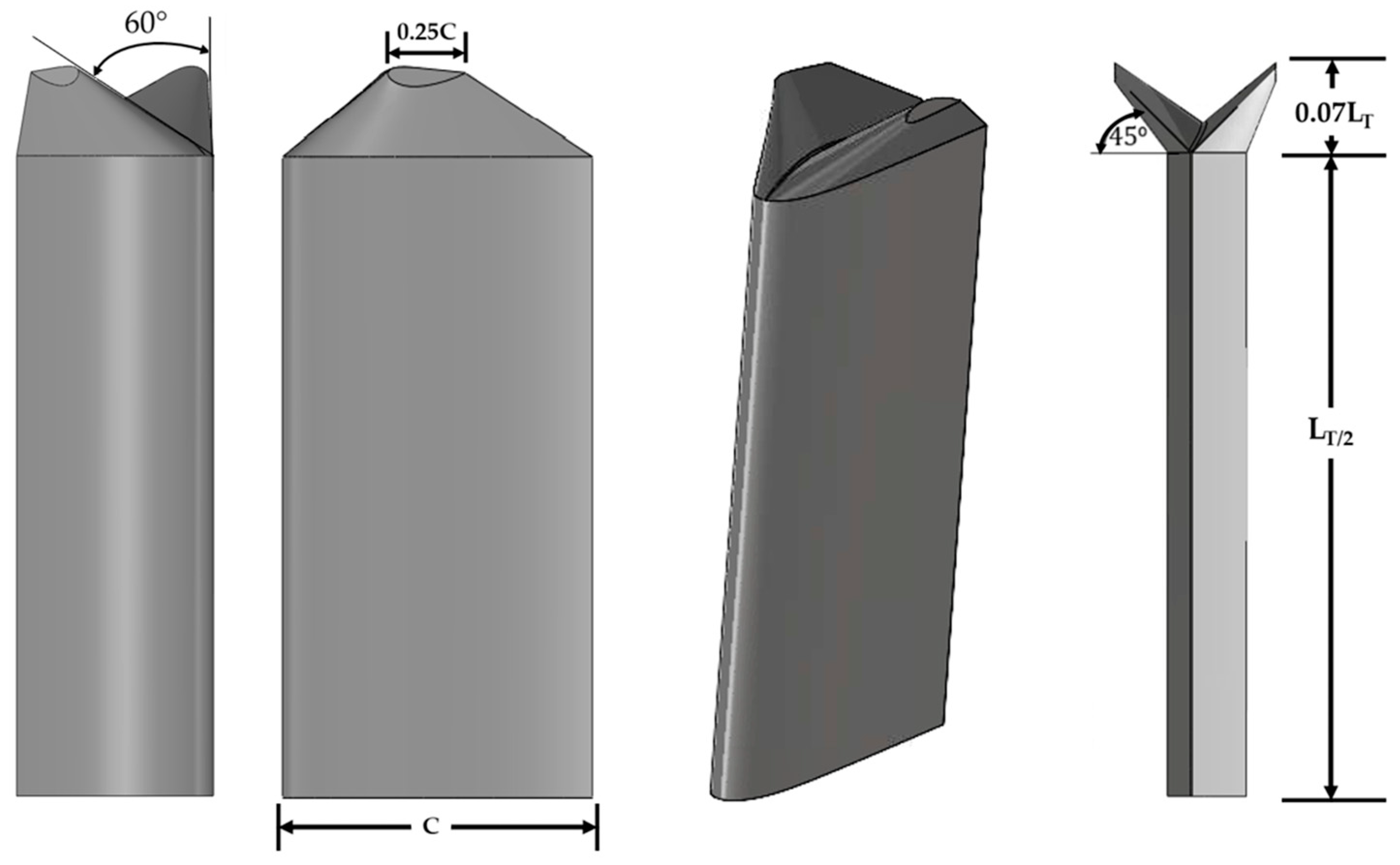
2.1. Geometric Model
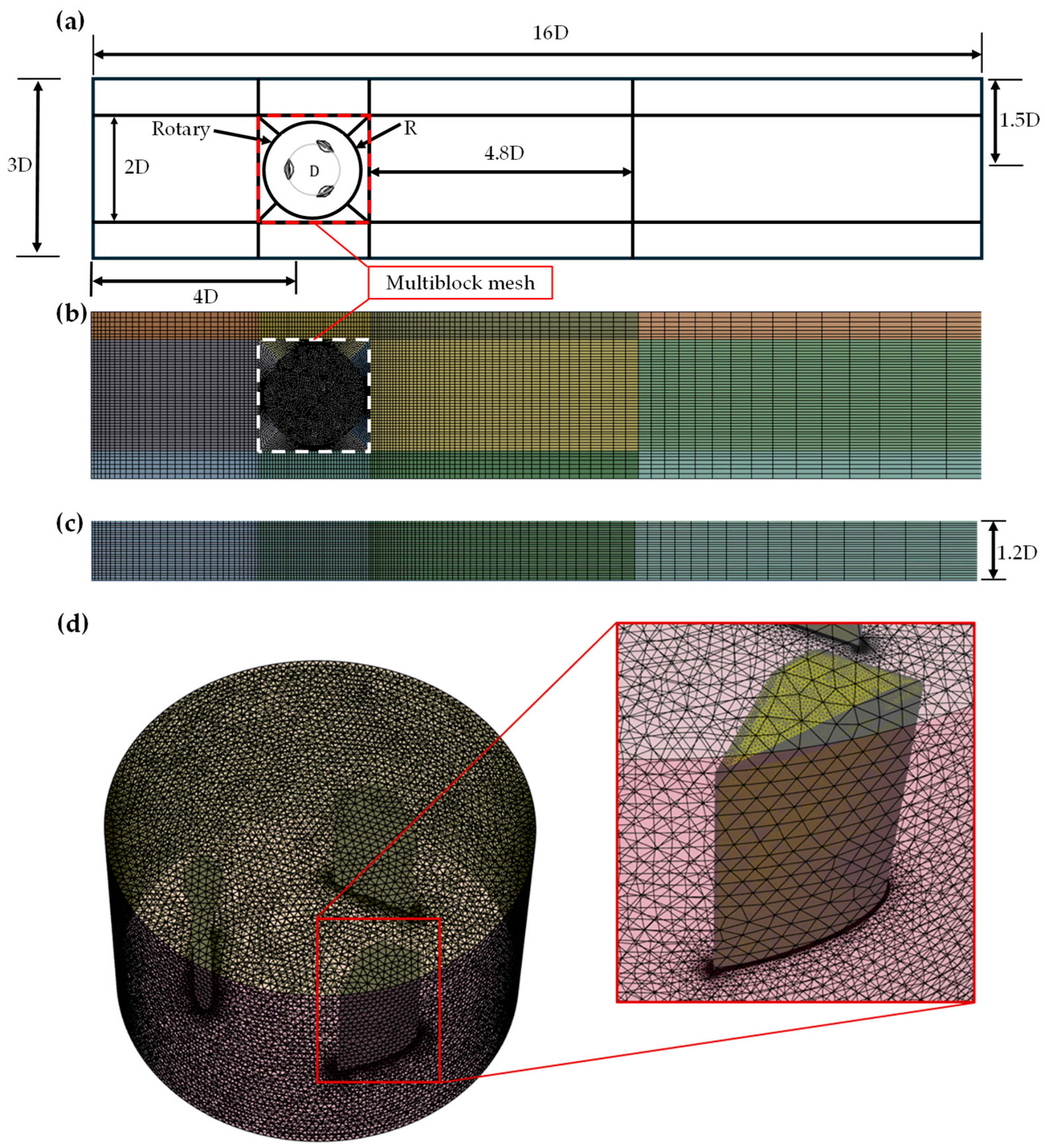
2.2. Numerical Configuration
3. Fluid–Structure Interaction (FSI) Approach
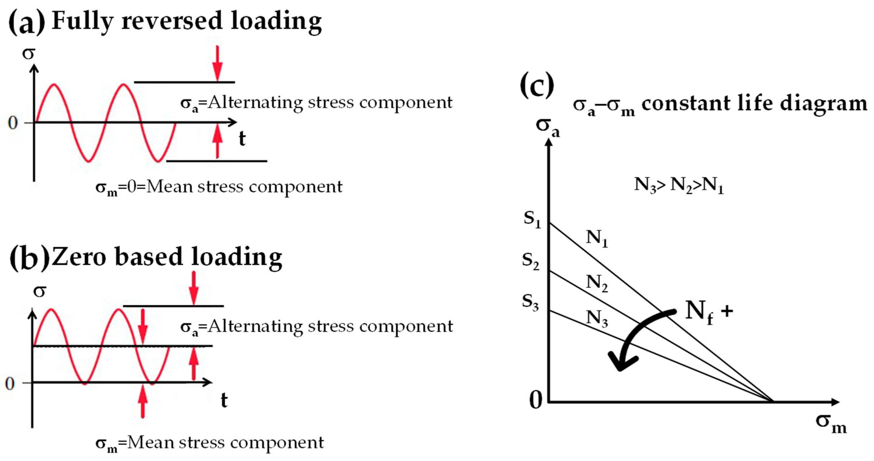
Fatigue Analysis
4. Results and Discussion
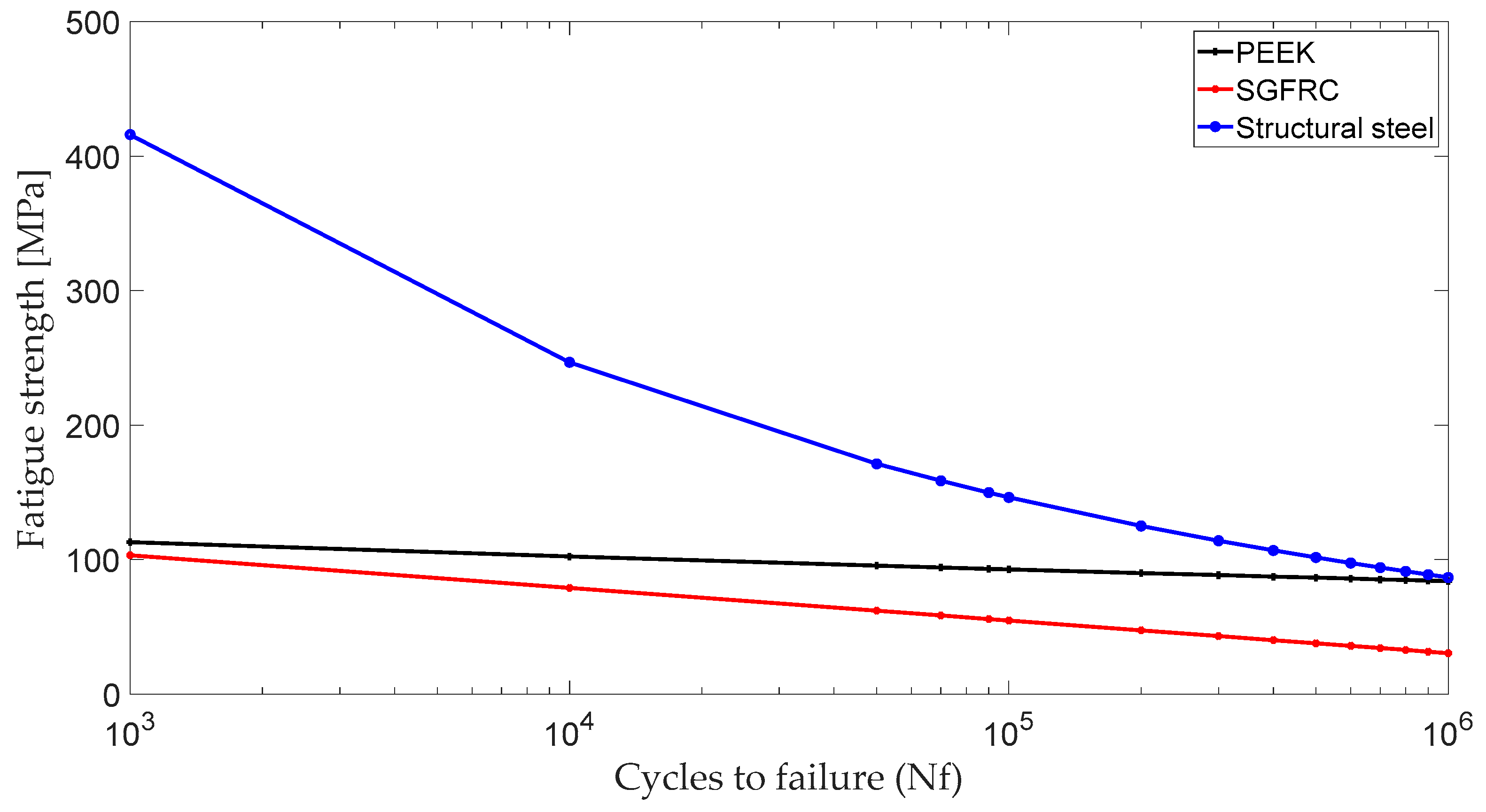
4.1. Fatigue Strength of the Materials
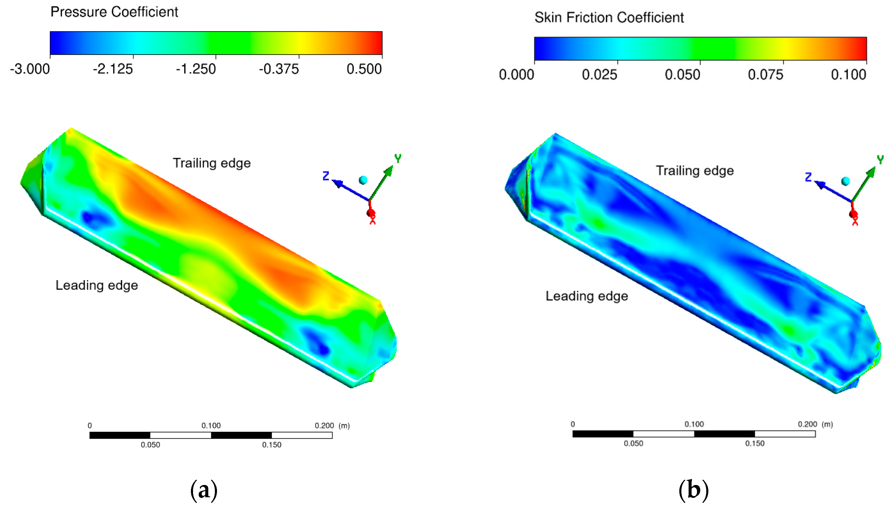
4.2. FSI Analysis of the VAH Straight-Bladed Darrieus Turbine with Winglets
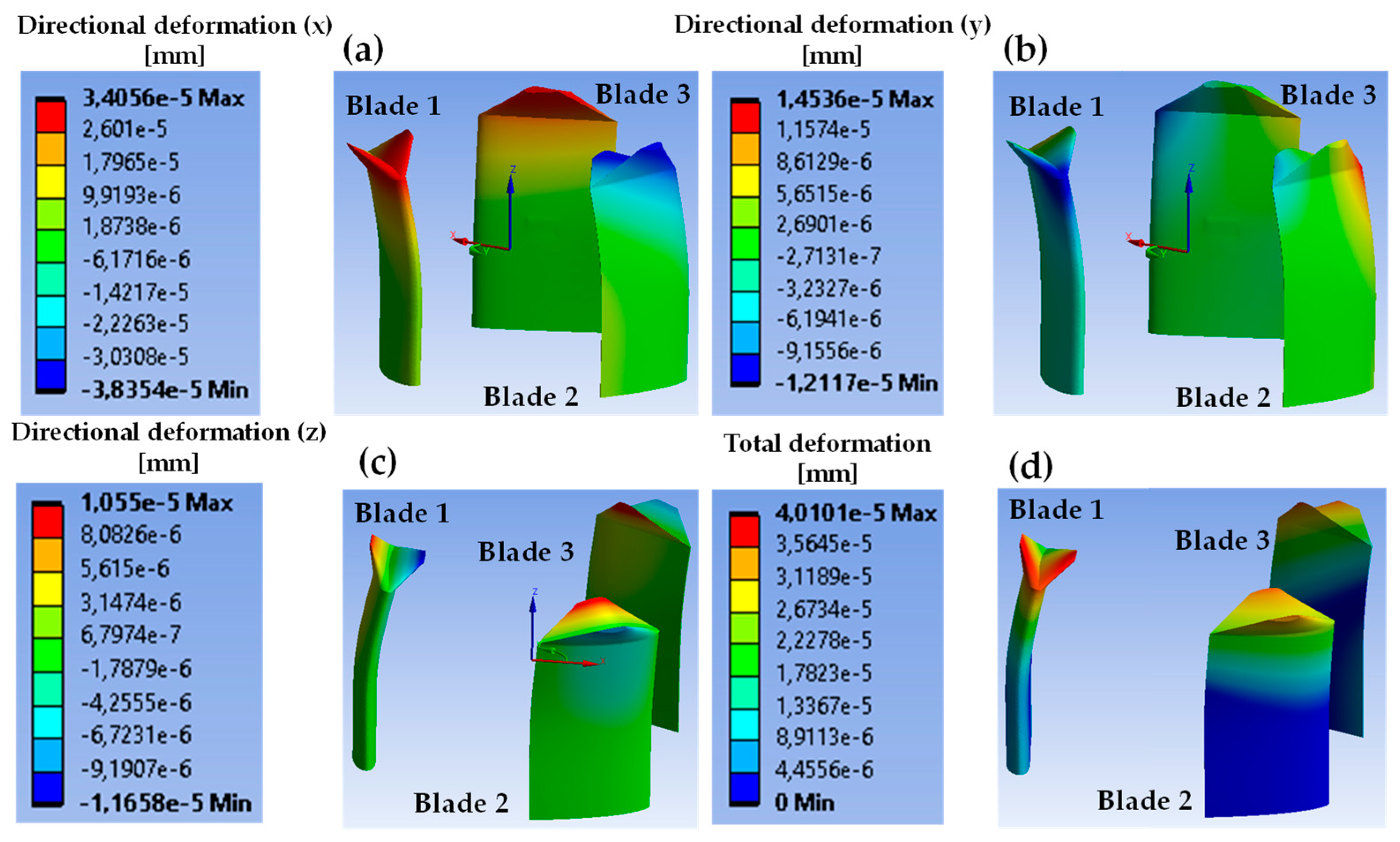
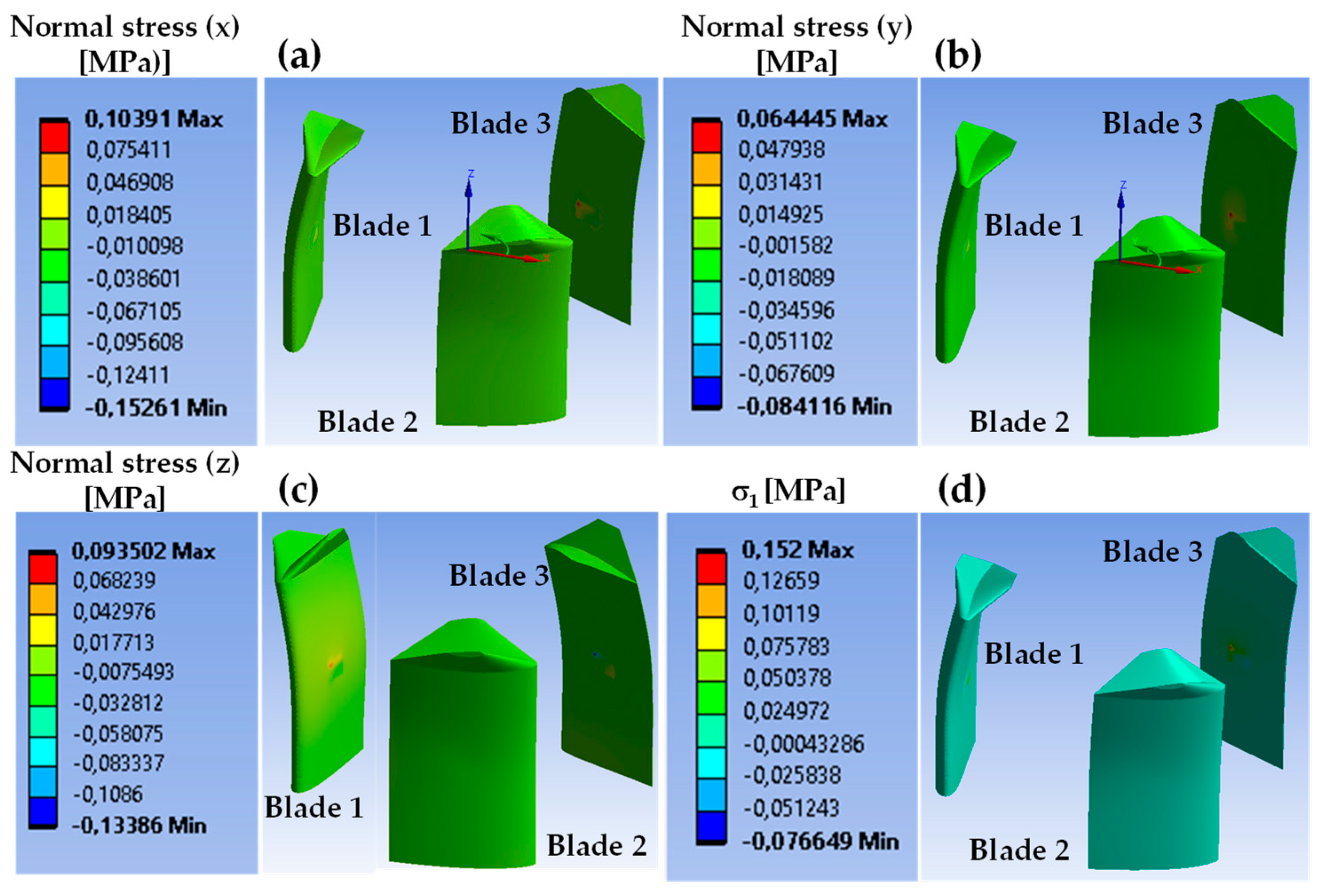
Structural and Fatigue Analysis
4.3. Modal Analysis
5. Summary and Conclusions
- The sliding mesh method was successfully employed to transfer the hydrodynamic loads to the VAHT blades to perform the FSI study using a cyclic zero-based fatigue loading with the Goodman theory and the S-N method.
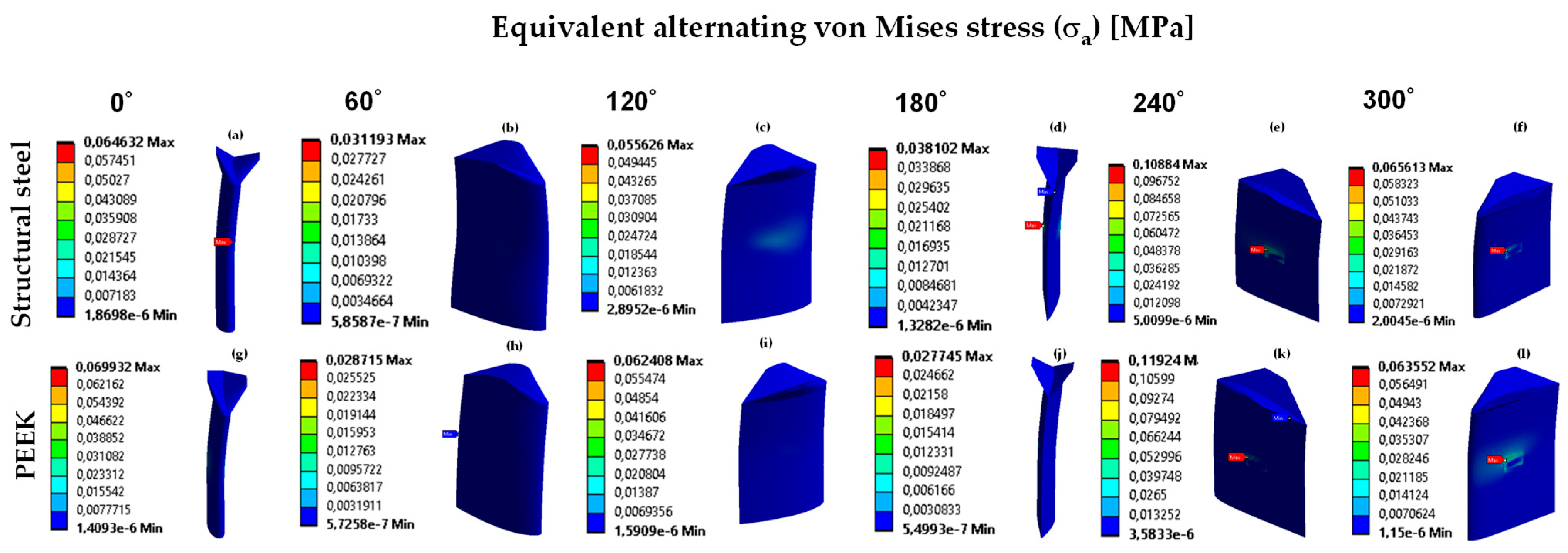
- Structural steel, SGFRC, and PEEK were used as materials to simulate the fatigue behavior of the VAHT blades. While SGFRC displayed poor structural behavior and fatigue resistance, structural steel and PEEK performed very well. Their equivalent alternating von Mises stresses remained well below their yield and fatigue strength during one azimuthal rotation, indicating an infinite fatigue life under the conditions of the current study. An equivalent alternating von Mises stress of half of the main principal stress was found during one azimuthal rotation, mainly related to the nature of the zero-based loading scenario ( = /2).
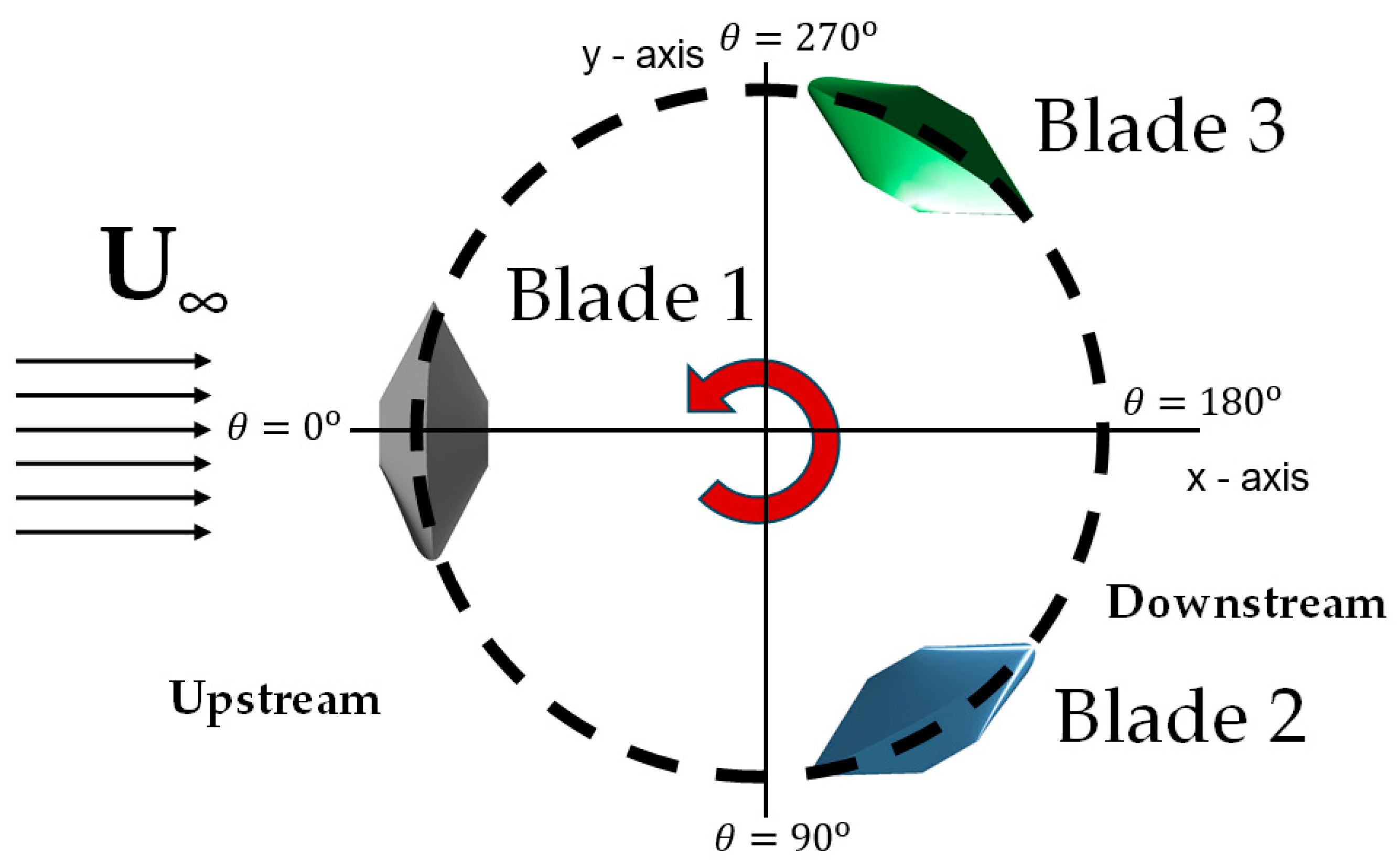
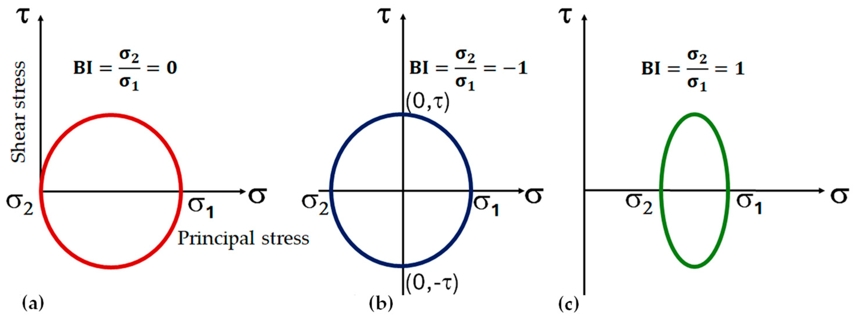
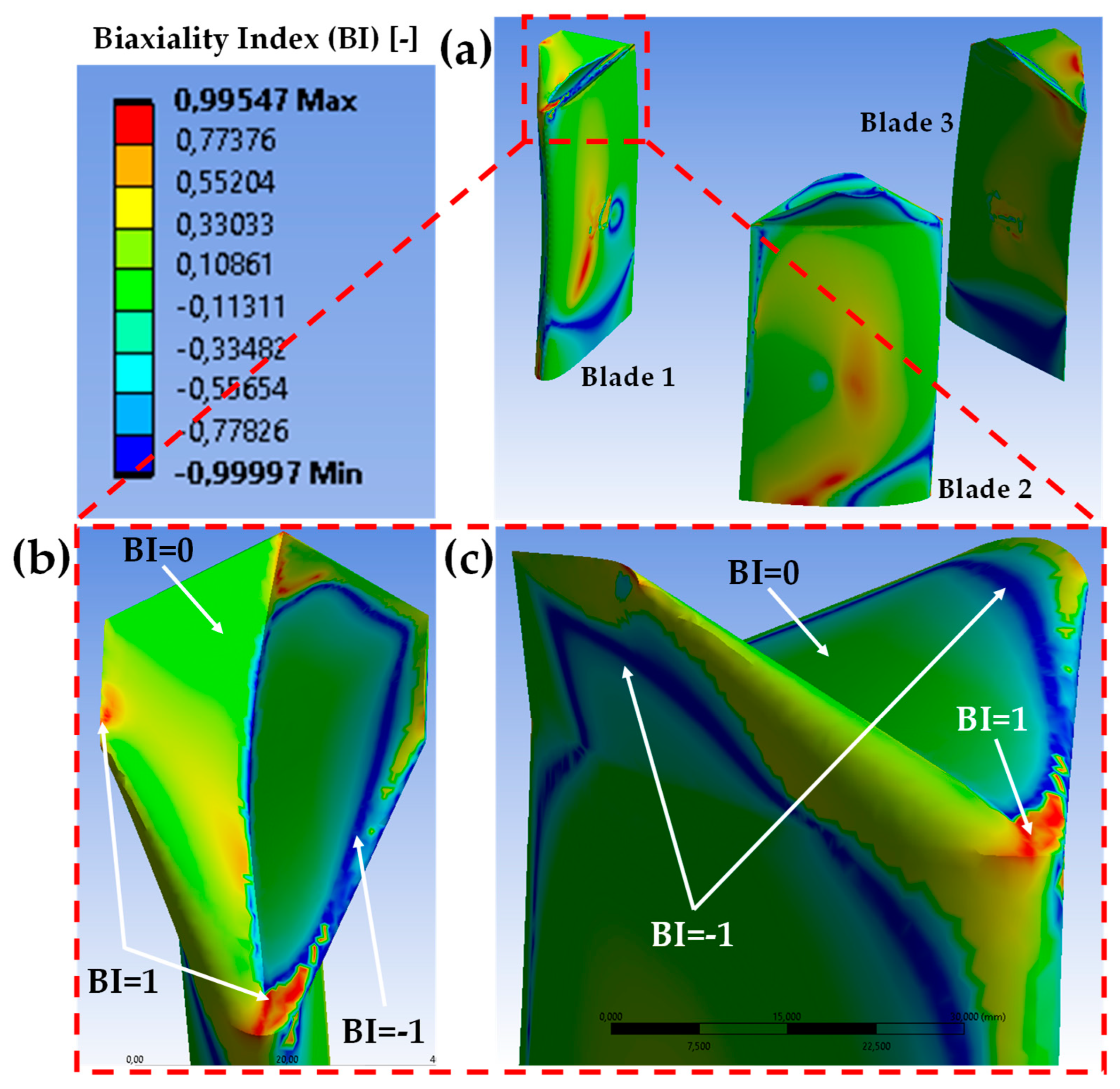
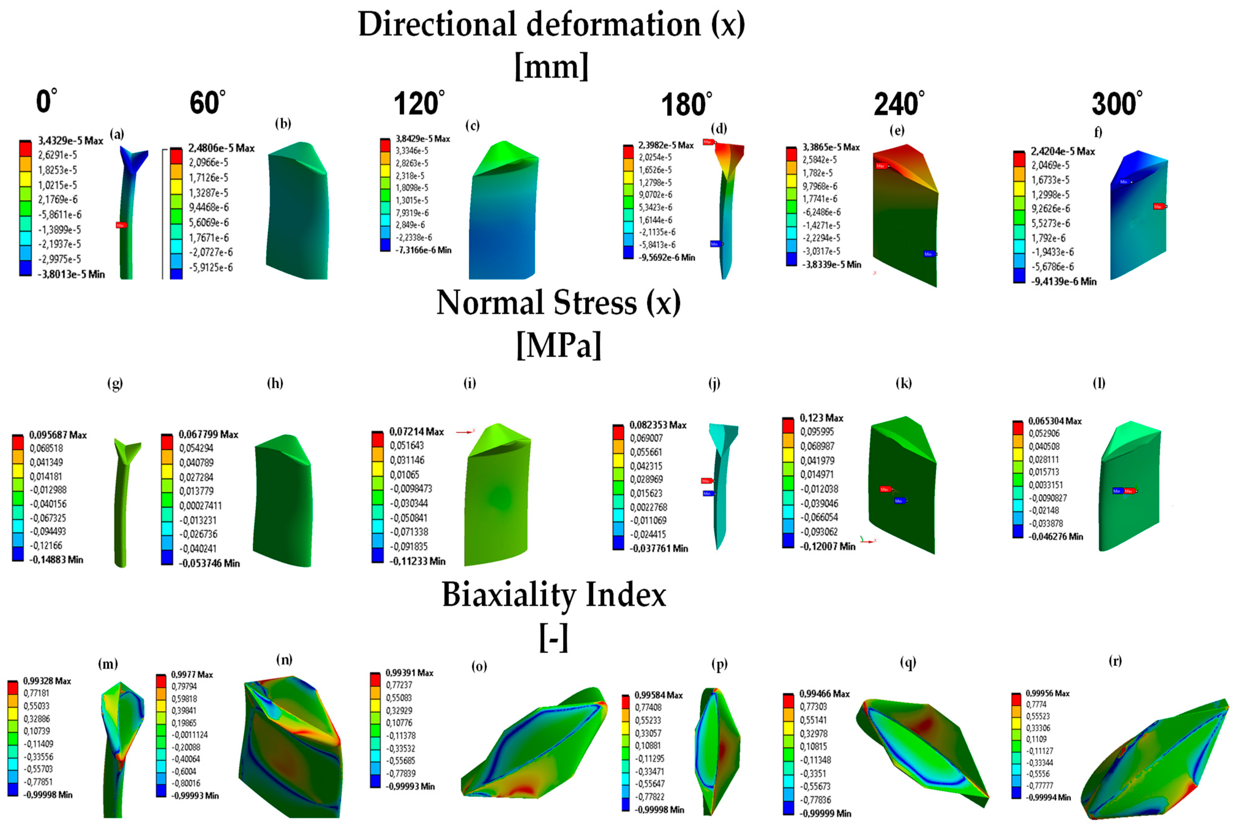
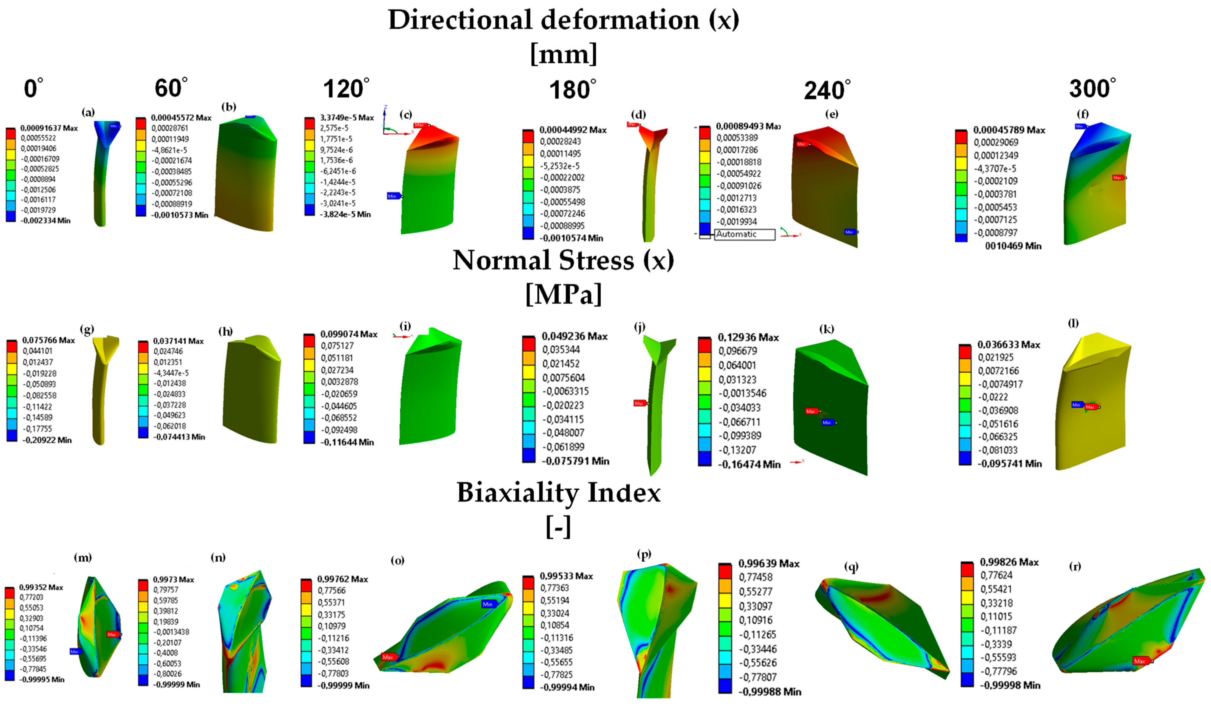
- The biaxiality index () was employed to understand the most dominant stresses in the winglet and the blade span regions during one azimuthal rotation. It was found that tension–compression bending stresses () were the predominant stresses along the blade, which operates as a cantilever beam under the current boundary conditions. However, shear stresses induced by the torsional moments and shedding vortex () were also observed in both regions (winglet and blade span), along with localized biaxial stresses. Unlike biaxial stresses (), which shift along the winglet’s surface with the blade’s azimuthal rotation, shear stresses only change between 120° and 240°. Variations in biaxial stresses are due to changes in the radial and tangential (or circumferential) normal stress components. In contrast, those of shear stresses are related to the variation of the lift and drag coefficients between 120° and 240°.
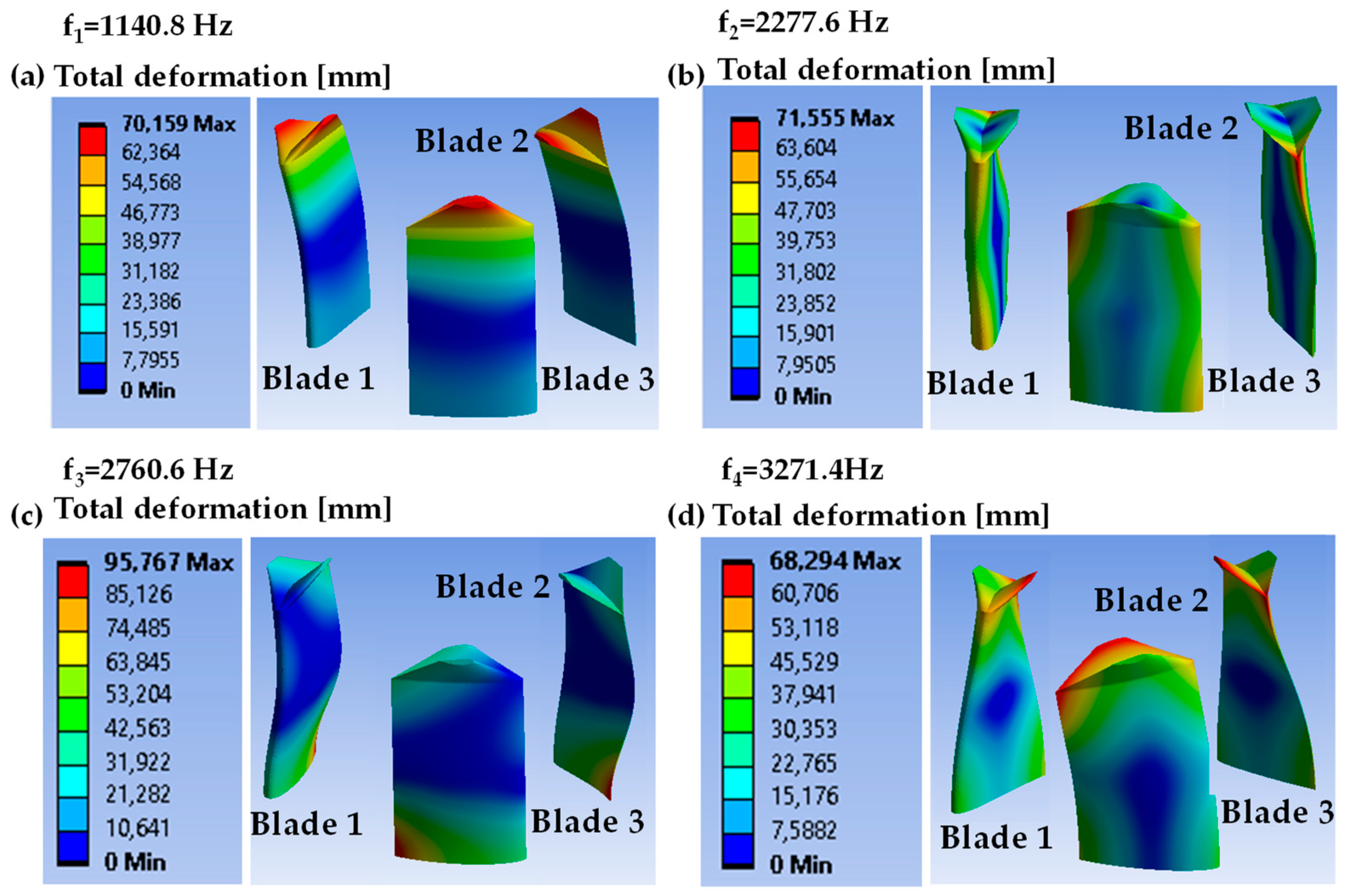
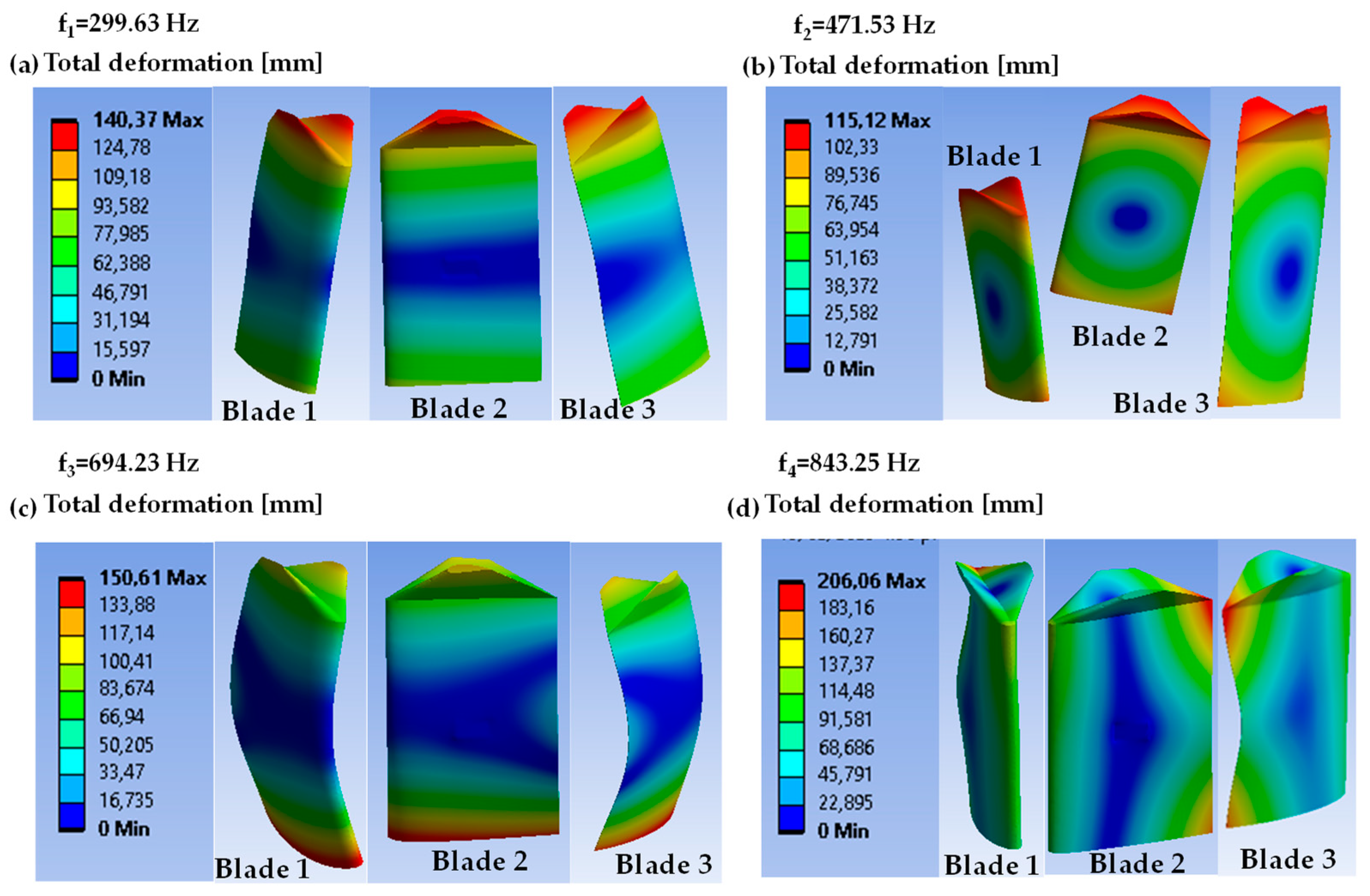
- The modal analysis of the blades in the first to fourth vibration modes of the best-performing materials (structural steel and PEEK) not only showed higher natural frequencies but also distinct bending, torsional, higher-order bending, and bending-torsional coupled modes for structural steel. Natural frequencies for PEEK were lower than those of structural steel, with the first and second modes having close values.
- Future experimental studies need to be performed to understand the effect of the added mass and the fluid damping on the dynamic response of the VAHT in the vicinity of resonance.
- Numerical simulations employing two-way coupling FSI are planned in the near future.
Author Contributions
Funding
Institutional Review Board Statement
Informed Consent Statement
Data Availability Statement
Acknowledgments
Conflicts of Interest
References
- Kusakana, K.; Vermaak, H.J. Hydrokinetic power generation for rural electricity supply: Case of South Africa. Renew. Energy 2023, 55, 467–473. [Google Scholar] [CrossRef]
- Niebuhr, C.M.; van Dijk, M.; Neary, M.V.; Bhagwan, J.N. A review of hydrokinetic turbines and enhancement techniques for canal installations: Technology, applicability and potential. Renew. Sustain. Energy Rev. 2019, 113, 109240. [Google Scholar] [CrossRef]
- Pandey, B.; Karki, A. Hydroelectric Energy: Renewable Energy and the Environment; CRC Press: Boca Raton, FL, USA, 2016. [Google Scholar] [CrossRef]
- Ridgill, M.; Neill, S.P.; Lewis, M.J.; Robins, P.E.; Patil, S.D. Global riverine theoretical hydrokinetic resource assessment. Renew. Energy 2021, 174, 654–665. [Google Scholar] [CrossRef]
- Zomers, A. The challenge of rural electrification. Energy Sustain. Dev. 2003, 7, 69–76. [Google Scholar] [CrossRef]
- Santos, L.F.S.D.; Camacho, R.G.R.; Tiago Filho, G.H.; Botan, A.C.B.; Vinent, B.A. Energy potential and economic analysis of hydrokinetic turbines implementation in rivers: An approach using numerical predictions (CFD) and experimental data. Renew. Energy 2019, 143, 648–662. [Google Scholar] [CrossRef]
- Henrique Da Costa Oliveira, C.; De Lourdes Cavalcanti Barros, M.; Alves Castelo Branco, D.; Soria, R.; Cesar Colonna Rosman, P. Evaluation of the hydraulic potential with hydrokinetic turbines for isolated systems in locations of the Amazon region. Sustain. Energy Technol. Assess. 2021, 45, 101079. [Google Scholar] [CrossRef]
- Lain, S.; Contreras, L.T.; López, O.D. A review on computational fluid dynamics modeling and simulation of horizontal axis hydrokinetic turbines. J. Braz. Soc. Mech. Sci. Eng. 2019, 41, 375. [Google Scholar] [CrossRef]
- Khan, M.J.; Bhuyan, G.; Iqbal, M.T.; Quaicoe, J.E. Hydrokinetic energy conversion systems and assessment of horizontal and vertical axis turbines for river and tidal applications: A technology status review. Appl. Energy 2009, 86, 1823–1835. [Google Scholar] [CrossRef]
- Vermaak, H.J.; Kusakana, K.; Koko, S.P. Status of micro-hydrokinetic river technology in rural applications: A review of literature. Renew. Sustain. Energy Rev. 2014, 29, 625–633. [Google Scholar] [CrossRef]
- Dewan, A.; Tomar, S.S.; Bishnoi, A.K.; Singh, T.P. Computational fluid dynamics and turbulence modelling in various blades of Savonius turbines for wind and hydro energy: Progress and perspectives. Ocean Eng. 2023, 283, 115168. [Google Scholar] [CrossRef]
- Ferrari, G.; Federici, D.; Schito, P.; Inzoli, F.; Mereu, R. CFD study of Savonius wind turbine: 3D model validation and parametric analysis. Renew. Energy 2017, 105, 722–734. [Google Scholar] [CrossRef]
- Alizadeh, H.; Jahangir, M.H.; Ghasempour, R. CFD-based improvement of Savonius type hydrokinetic turbine using optimized barrier at the low-speed flows. Ocean Eng. 2020, 202, 107178. [Google Scholar] [CrossRef]
- Tantichukiad, K.; Yahya, A.; Mohd Mustafah, A.; Mohd Rafie, A.S.; Mat Su, A.S. Design evaluation reviews on the savonius, darrieus, and combined savonius-darrieus turbines. Proc. Inst. Mech. Eng. Part A J. Power Energy 2023, 237, 1348–1366. [Google Scholar] [CrossRef]
- Kamal, M.M.; Saini, R.P. A numerical investigation on the influence of savonius blade helicity on the performance characteristics of hybrid cross-flow hydrokinetic turbine. Renew. Energy 2022, 190, 788–804. [Google Scholar] [CrossRef]
- Patel, V.; Eldho, T.I.; Prabhu, S.V. Experimental investigations on Darrieus straight blade turbine for tidal current application and parametric optimization for hydro farm arrangement. Int. J. Mar. Energy 2017, 17, 110–135. [Google Scholar] [CrossRef]
- Buchner, A.J.; Soria, J.; Honnery, D.; Smits, A.J. Dynamic stall in vertical axis wind turbines: Scaling and topological considerations. J. Fluid Mech. 2018, 841, 746–766. [Google Scholar] [CrossRef]
- López, O.D.; Mejía, O.E.; Escorcia, K.M.; Suárez, F.; Lain, S. Comparison of sliding and overset mesh techniques in the simulation of a vertical axis turbine for hydrokinetic applications. Processes 2021, 9, 1933. [Google Scholar] [CrossRef]
- Raciti Castelli, M.; Englaro, A.; Benini, E. The Darrieus wind turbine: Proposal for a new performance prediction model based on CFD. Energy 2011, 36, 4919–4934. [Google Scholar] [CrossRef]
- Nobile, R.; Vahdati, M.; Barlow, J.F.; Mewburn-Crook, A. Unsteady flow simulation of a vertical axis augmented wind turbine: A two-dimensional study. J. Wind. Eng. Ind. Aerodyn. 2014, 125, 168–179. [Google Scholar] [CrossRef]
- Ramesh, K.; Gopalarathnam, A.; Granlund, K.; Ol, M.V.; Edwards, J.R. Discrete-vortex method with novel shedding criterion for unsteady aerofoil flows with intermittent leading-edge vortex shedding. J. Fluid Mech. 2014, 751, 500–538. [Google Scholar] [CrossRef]
- Hoerner, S.; Abbaszadeh, S.; Maître, T.; Cleynen, O.; Thévenin, D. Characteristics of the fluid–structure interaction within Darrieus water turbines with highly flexible blades. J. Fluids Struct. 2019, 88, 13–30. [Google Scholar] [CrossRef]
- Ghiss, M.; Bahri, Y.; Souaissa, K.; Troudi, H.; Ting, D.S.K.; Tourki, Z. Enhancing Vertical Axis Wind Turbine Performance Using Winglets. In International Conference Design and Modeling of Mechanical Systems; Springer: Cham, Switzerland, 2021; pp. 323–334. [Google Scholar] [CrossRef]
- Xu, W.; Li, G.; Wang, F.; Li, Y. High-resolution numerical investigation into the effects of winglet on the aerodynamic performance for a three-dimensional vertical axis wind turbine. Energy Convers. Manag. 2020, 205, 112333. [Google Scholar] [CrossRef]
- Narayan, G.; John, B.B. Effect of winglets induced tip vortex structure on the performance of subsonic wings. Aerosp. Sci. Technol. 2016, 58, 328–340. [Google Scholar] [CrossRef]
- Lain, S.; Taborda, M.A.; López, O.D. Numerical Study of the Effect of Winglets on the Performance of a Straight Blade Darrieus Water Turbine. Energies 2018, 11, 297. [Google Scholar] [CrossRef]
- Guillaud, N.; Balarac, G.; Goncalvès, E.; Zanette, J. Large Eddy Simulations on Vertical Axis Hydrokinetic Turbines-Power coefficient analysis for various solidities. Renew. Energy 2020, 147, 473–486. [Google Scholar] [CrossRef]
- Ye, J.; Zhou, H.; He, K. A generalized framework of two-way coupled numerical model for fluid-structure-seabed interaction (FSSI): Explicit algorithm. Eng. Geol. 2024, 340, 107679. [Google Scholar] [CrossRef]
- Hoseini, S.S.; Najafi, G.; Ghobadian, B.; Akbarzadeh, A.H. Impeller shape-optimization of stirred-tank reactor: CFD and fluid structure interaction analyses. Chem. Eng. J. 2021, 413, 127497. [Google Scholar] [CrossRef]
- Benra, F.K.; Dohmen, H.J.; Pei, J.; Schuster, S.; Wan, B. A Comparison of One-Way and Two-Way Coupling Methods for Numerical Analysis of Fluid-Structure Interactions. J. Appl. Math. 2011, 2011, 853560. [Google Scholar] [CrossRef]
- Li, F.; Fu, J.; Chen, J.; Hu, D. Two-way coupling fluid–structure interaction analysis on dynamic response of offshore wind turbine. Mar. Georesources Geotechnol. 2024, 42, 1677–1686. [Google Scholar] [CrossRef]
- Dörfler, P.; Sick, M.; Coutu, A. Flow-Induced Pulsation and Vibration in Hydroelectric Machinery, 1st ed.; Springer: Berlin/Heidelberg, Germany, 2013. [Google Scholar] [CrossRef]
- Pozarlik, A.K.; Kok, J.B.W. Numerical investigation of one- and two-way fluid-structure interaction in combustion systems. In International Conference on Computational Methods for Coupled Problems in Science and Engineering–COUPLED PROBLEMS; CIMNE: Barcelona, Spain, 2007; pp. 610–614. [Google Scholar]
- Wang, L.; Quant, R.; Kolios, A. Fluid structure interaction modelling of horizontal-axis wind turbine blades based on CFD and FEA. J. Wind. Eng. Ind. Aerodyn. 2016, 158, 11–25. [Google Scholar] [CrossRef]
- Kang, Y.S.; Sohn, D.; Kim, J.H.; Kim, H.G.; Im, S. A sliding mesh technique for the finite element simulation of fluid–solid interaction problems by using variable-node elements. Comput. Struct. 2014, 130, 91–104. [Google Scholar] [CrossRef]
- Trivedi, C. A review on fluid structure interaction in hydraulic turbines: A focus on hydrodynamic damping. Eng. Fail. Anal. 2017, 77, 1–22. [Google Scholar] [CrossRef]
- López, O.D.; Botero, N.; Nunez, E.E.; Lain, S. Performance Improvement of a Straight-Bladed Darrieus Hydrokinetic Turbine through Enhanced Winglet Designs. J. Mar. Sci. Technol. 2024, 12, 977. [Google Scholar] [CrossRef]
- Yagmur, S.; Kose, F.; Dogan, S. A study on performance and flow characteristics of single and double H-type Darrieus turbine for a hydro farm application. Energy Convers. Manag. 2021, 245, 114599. [Google Scholar] [CrossRef]
- Rezaeiha, A.; Kalkman, I.; Blocken, B. CFD simulation of a vertical axis wind turbine operating at a moderate tip speed ratio: Guidelines for minimum domain size and azimuthal increment. Renew. Energy 2017, 107, 373–385. [Google Scholar] [CrossRef]
- Langtry, R.B.; Menter, F.R. Correlation-Based Transition Modeling for Unstructured Parallelized Computational Fluid Dynamics Codes. AIAA J. 2009, 47, 2894–2906. [Google Scholar] [CrossRef]
- Menter, F.R. Review of the shear-stress transport turbulence model experience from an industrial perspective. Int. J. Comput. Fluid Dyn. 2009, 23, 305–316. [Google Scholar] [CrossRef]
- Badshah, M.; Badshah, S.; VanZwieten, J.; Jan, S.; Amir, M.; Malik, S.A. Coupled Fluid-Structure Interaction Modelling of Loads Variation and Fatigue Life of a Full-Scale Tidal Turbine under the Effect of Velocity Profile. Energies 2019, 12, 2217. [Google Scholar] [CrossRef]
- Biswas, R.; Sharma, N.; Singh, K.K. Numerical analysis of mechanical and fatigue behaviour of glass and carbon fibre reinforced polymer composite. Mater. Today Proc. 2023, 3, 479. [Google Scholar] [CrossRef]
- Shrestha, R.; Simsiriwong, J.; Shamsaei, N.; Moser, R.D. Cyclic deformation and fatigue behavior of polyether ether ketone (PEEK). Int. J. Fatigue 2016, 82, 411–427. [Google Scholar] [CrossRef]
- Rae, P.J.; Brown, E.N.; Orler, E.B. The mechanical properties of poly(ether-ether-ketone) (PEEK) with emphasis on the large compressive strain response. Polymer 2007, 48, 598–615. [Google Scholar] [CrossRef]
- Nunez, E.E.; Gheisari, R.; Polycarpou, A.A. Tribology review of blended bulk polymers and their coatings for high-load bearing applications. Tribol. Int. 2019, 129, 92–111. [Google Scholar] [CrossRef]
- Chen, F.; Gatea, S.; Ou, H.; Lu, B.; Long, H. Fracture characteristics of PEEK at various stress triaxialities. J. Mech. Behav. Biomed. Mater. 2016, 64, 173–186. [Google Scholar] [CrossRef]
- Abbasnezhad, N.; Khavandi, A.; Fitoussi, J.; Arabi, H.; Shirinbayan, M.; Tcharkhtchi, A. Influence of loading conditions on the overall mechanical behavior of polyether-ether-ketone (PEEK). Int. J. Fatigue 2018, 109, 83–92. [Google Scholar] [CrossRef]
- Zago, A.; Springer, G.S. Constant Amplitude Fatigue of Short Glass and Carbon Fiber Reinforced Thermoplastics. J. Reinf. Plast. Compos. 2001, 20, 564–595. [Google Scholar] [CrossRef]
- Mortazavian, S.; Fatemi, A. Fatigue behavior and modeling of short fiber reinforced polymer composites: A literature review. Int. J. Fatigue 2015, 70, 297–321. [Google Scholar] [CrossRef]
- Trivedi, C.; Cervantes, M.J. Fluid-structure interactions in Francis turbines: A perspective review. Renew. Sustain. Energy Rev. 2017, 68, 87–101. [Google Scholar] [CrossRef]
- Ali, S.; Park, H.; Lee, D. Structural Optimization of Vertical Axis Wind Turbine (VAWT): A Multi-Variable Study for Enhanced Deflection and Fatigue Performance. J. Mar. Sci. Eng. 2025, 13, 19. [Google Scholar] [CrossRef]
- Cao, J.; Luo, Y.; Liu, X.; Presas, A.; Deng, L.; Zhao, W.; Xia, M.; Wang, Z. Numerical theory and method on the modal behavior of a pump-turbine rotor system considering gyro-effect and added mass effect. J. Energy Storage 2024, 85, 111064. [Google Scholar] [CrossRef]
- Luo, W.; Liu, W.; Chen, S.; Zou, Q.; Song, X. Development and Application of an FSI Model for Floating VAWT by Coupling CFD and FEA. J. Mar. Sci. Eng. 2024, 12, 4. [Google Scholar] [CrossRef]
- Urban, O.; Pochylý, F.; Habán, V. Estimation of added effects and their frequency dependence in various fluid–structure interaction problems. J. Braz. Soc. Mech. Sci. Eng. 2024, 46, 631. [Google Scholar] [CrossRef]
- Guo, Y.; Yang, W.; Dong, Y.; Xue, D. Resonance mechanism of flapping wing based on fluid structure interaction simulation. Chin. J. Aeronaut. 2024, 37, 243–262. [Google Scholar] [CrossRef]
- Yusuf, A.O.; Hasan, M.A.; Khalil, E. Vibration mitigation of wind turbines with tuned liquid damper using fluid-structure coupling analysis. Int. J. Dynam. Control 2024, 12, 3517–3533. [Google Scholar] [CrossRef]
- Lain, S.; Garcia, M.J.; Quintero, B.; Orrego, S. CFD numerical simulations of Francis turbines. Rev. Fac. Ing. Univ. Antioquia 2010, 51, 31–40. [Google Scholar] [CrossRef]


| Parameter | Value |
|---|---|
| Blade profile | NACA4418 |
| Turbine diameter [] | 0.25 m |
| Blade span [] | 0.3 m |
| Chord length [] | 0.1 m |
| Number of blades | 3 |
| Solidity | 2.4 |
| Parameter | Value |
|---|---|
| Width of the domain (W) | 3D |
| Length of the fluid domain (L) | 16D |
| Height of the fluid domain (H) | 1.2D |
| Distance from the wall to the center of the turbine (w) | 1.5D |
| Distance from the inlet to the center of the turbine (l) | 4D |
| Mesh refinement near the turbine (R) | 1.8D |
| Square prism enclosing the rotating subdomain () | 2D |
| Parameter | Value |
|---|---|
| Free-stream Velocity [] | 0.3 m/s |
| Turbine Angular Velocity [] at | 2.4 rad/s |
| Time step | 0.0036 s |
| Iterations per time step | 75 |
| Residuals convergence criterion | |
| Time discretization | Second order implicit |
| Spatial discretization | Second order upwind |
| SS | SGFRC | PEEK | |
|---|---|---|---|
| Density (kg/m3) | 7850 | 1600 | 1300 |
| Poisson’s ratio | 0.28 | 0.37 | 0.38 |
| Young’s modulus (GPa) | 207 | 10 | 4.4 |
| Tensile yield strength (MPa) | 250 | 70 | 110 |
| Ultimate tensile strength (MPa) | 460 | 178.5 | 117 |
| Fatigue strength at (MPa) | 86 | 30.34 | 84 |
Disclaimer/Publisher’s Note: The statements, opinions and data contained in all publications are solely those of the individual author(s) and contributor(s) and not of MDPI and/or the editor(s). MDPI and/or the editor(s) disclaim responsibility for any injury to people or property resulting from any ideas, methods, instructions or products referred to in the content. |
© 2025 by the authors. Licensee MDPI, Basel, Switzerland. This article is an open access article distributed under the terms and conditions of the Creative Commons Attribution (CC BY) license (https://creativecommons.org/licenses/by/4.0/).
Share and Cite
Nunez, E.E.; García González, D.; López, O.D.; Casas Rodríguez, J.P.; Laín, S. Fluid–Structure Interaction of a Darrieus-Type Hydrokinetic Turbine Modified with Winglets. J. Mar. Sci. Eng. 2025, 13, 548. https://doi.org/10.3390/jmse13030548
Nunez EE, García González D, López OD, Casas Rodríguez JP, Laín S. Fluid–Structure Interaction of a Darrieus-Type Hydrokinetic Turbine Modified with Winglets. Journal of Marine Science and Engineering. 2025; 13(3):548. https://doi.org/10.3390/jmse13030548
Chicago/Turabian StyleNunez, Emerson Escobar, Diego García González, Omar Darío López, Juan Pablo Casas Rodríguez, and Santiago Laín. 2025. "Fluid–Structure Interaction of a Darrieus-Type Hydrokinetic Turbine Modified with Winglets" Journal of Marine Science and Engineering 13, no. 3: 548. https://doi.org/10.3390/jmse13030548
APA StyleNunez, E. E., García González, D., López, O. D., Casas Rodríguez, J. P., & Laín, S. (2025). Fluid–Structure Interaction of a Darrieus-Type Hydrokinetic Turbine Modified with Winglets. Journal of Marine Science and Engineering, 13(3), 548. https://doi.org/10.3390/jmse13030548