ShipNetSim: An Open-Source Simulator for Real-Time Energy Consumption and Emission Analysis in Large-Scale Maritime Networks


Abstract
:1. Introduction
2. Literature Review
3. Novelty and Contributions
3.1. Comprehensive Multi-Domain Simulation
- Propulsion and Resistance Modeling: ShipNetSim utilizes advanced hydrodynamic models such as Holtrop method and B-Series thrust and torque coefficients to model the resistance forces on a ship with high accuracy under different environmental conditions.
- Dynamic Ship-Following Models: The simulator, incorporating principles of traffic flow theory, possesses an advanced ship-following model that takes into consideration vessel spacing, operators’ response delays, and braking dynamics, thus simulating longitudinal behavior realistically.
- Path Finding and Interaction with the Environment: Supported by a visibility graph data structure combined with QuadTree indexing, ShipNetSim simulates path planning through complicated maritime environments effectively, with the incorporation of variable environment parameters (such as wave properties and wind resistance).
- Cybersecurity Simulation: A new module simulates cyber threats like GPS spoofing, network attacks, and signal jamming to challenge the resilience of maritime operations to cyber disruptions.
3.2. Real-Time, Data-Driven Analysis
- Provide real-time measurement of energy use and emissions.
- Enable sensitivity analyses through examination of how monthly environmental changes contribute to operational effectiveness.
- Offer actionable suggestions for optimizing ship performance in different operating conditions.
3.3. Relevance to Decarbonisation and Policy Adherence
- Quantification of different operational measures impacts, such as speed adjustments, optimized routing, or alternative fuel utilization, on fuel consumption and CO2 emissions.
- Scenario analysis that enables companies to adhere to global decarbonization targets (such as those established by the IMO) by examining emission reduction strategies and their effectiveness.
- An experimental platform for innovative decarbonization measurements, for example, introducing renewable energy sources or hybrid propulsion systems. This thus supports operational improvements and policy formulation.
3.4. Modularity, Extensibility, and Future Communication Capabilities
- Lateral Dynamics Integration: An extension of the simulation framework to model lateral movements of ships and more intricate maneuvering patterns.
- Advanced Cyber Threat Frameworks: Incorporating machine learning algorithms for predictive analytics to enable cybersecurity evaluations to be more impactful.
- Better Energy Modeling: Incorporating auxiliary systems, additional fuel types, and more extensive engine performance readings.
- Communication Between Vessels and Shore Facilities: There is a need to develop modules that enable real-time interactions between maritime vessels and also between vessels and shore facilities. These capabilities would enable synchronized navigation, adaptive decision-making processes, and timely emergency responses, thus enhancing the operational realism and feasibility of the simulator.
3.5. Validation and Practical Impact
- Operational optimization and route planning.
- Environmental impact assessments.
- Strategic planning for decarbonization in maritime transport.
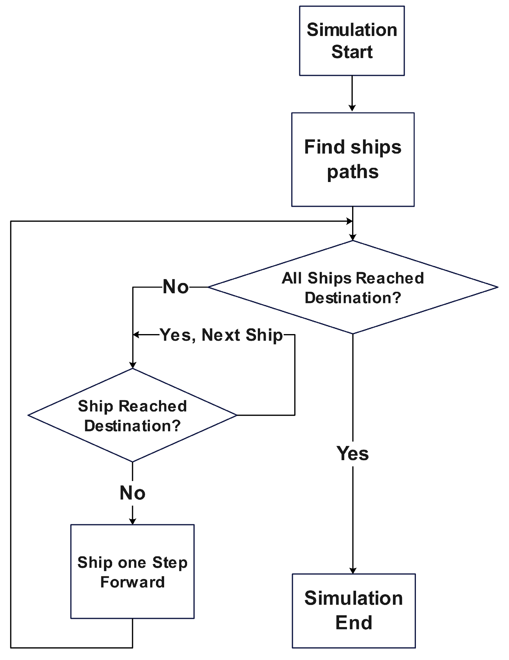
4. Simulation Model
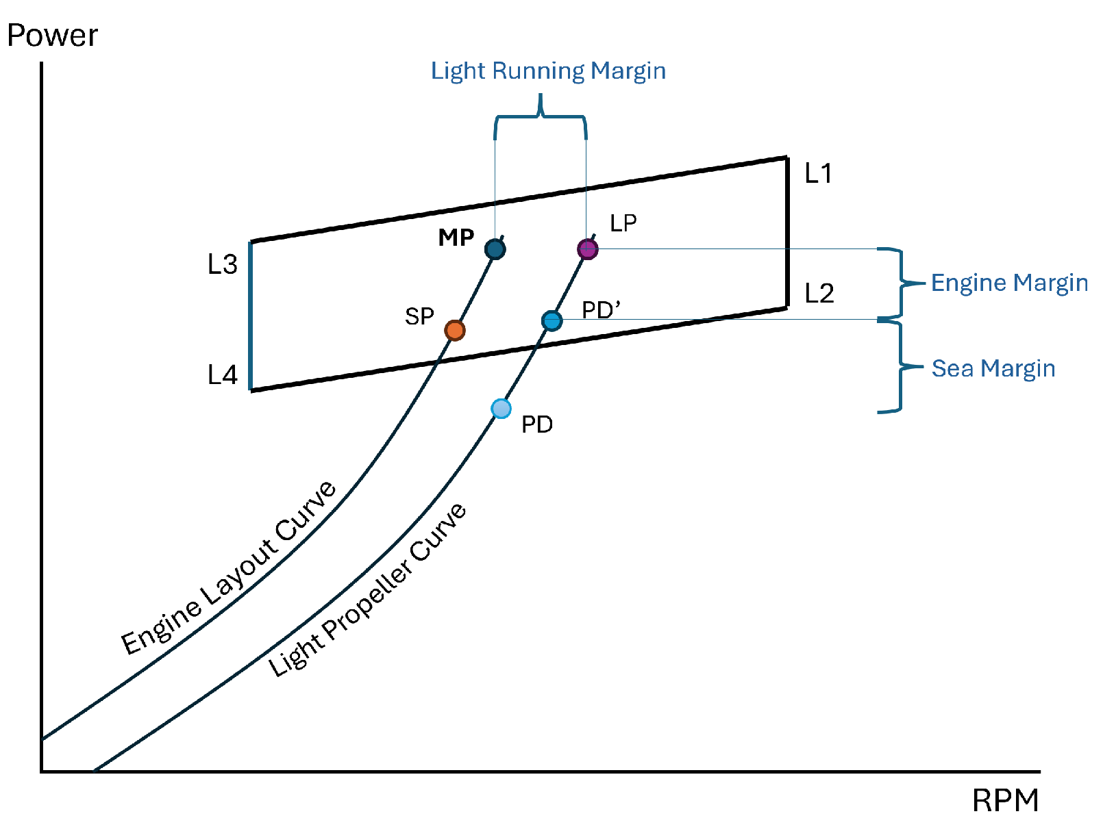
4.1. Propulsion-Resistance Models
4.2. Ship Motion and Coexisting Models
4.3. Visibility Graph Modelling and Path Finding
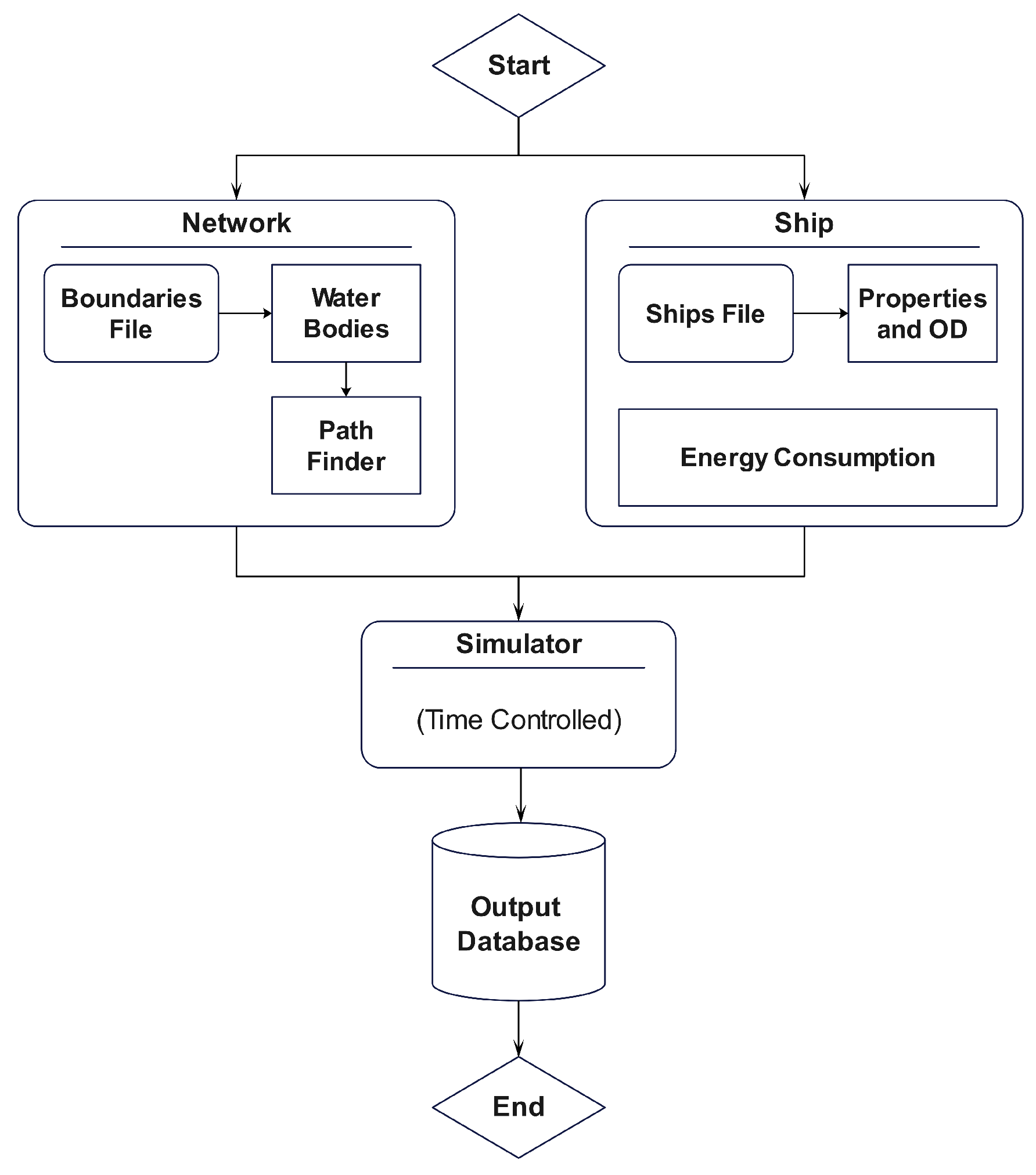
5. Simulator Description
Cybersecurity Simulation
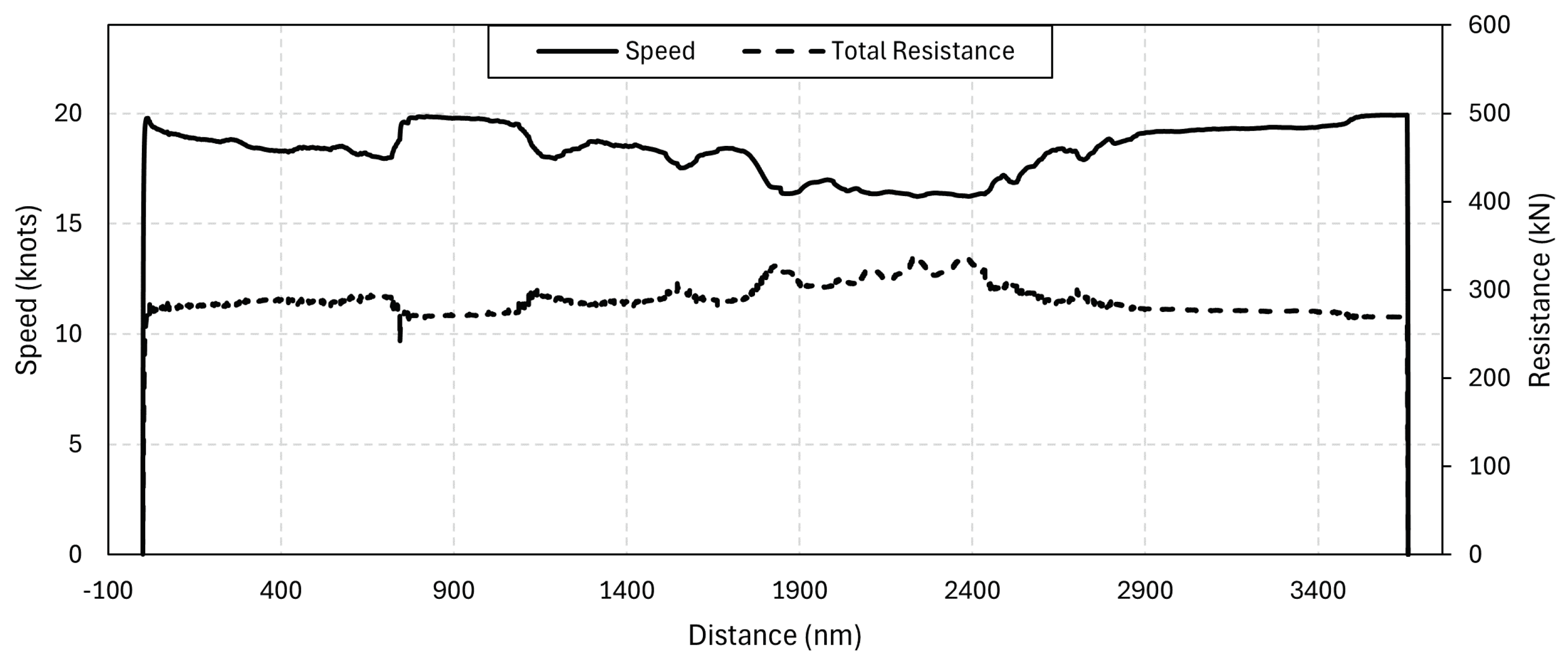
6. Case Studies
6.1. Environment Sensitivity Analysis
6.2. Discussion and Comparison
6.3. Analysis of Model Uncertainties
- Variability of Environmental Data: The simulation relies on environmental data (e.g., geospatial tiff files for wind and wave parameters) that inherently contain measurement errors and temporal/spatial variability.
- Model Parameter Calibration: Key parameters like the calibration coefficients (, , ) and the form factor () are derived from empirical data and literature values, which can be different in operating conditions.
- Numerical Approximations: The use of discrete time steps () and numerical integration techniques can lead to approximation errors.
7. Conclusions
Author Contributions
Funding
Data Availability Statement
Conflicts of Interest
Abbreviations
| Variable | Definition |
| Smoothed acceleration of ship n at instant t (m/s2) | |
| Acceleration of ship n at instant t (m/s2) | |
| B | Ship Beam (m) |
| Propulsion force of ship n at instant t (N) | |
| The Froude number at instant t | |
| Maximum engine power of the main engine (kW) | |
| The time it takes to deactivate the propulsion thrust or revert the propeller rotating direction plus the operator perception reaction time (s) | |
| The ship length between perpendiculars (m) | |
| m | Total mass of the vessel (kg) |
| Total Resistive forces at instant t (N) | |
| The calm water resistance component at instant t (N) | |
| The added resistance component due to waves of frequency and wave heading angle at instant t (N) | |
| The added resistance component due to wave reflection with wave frequency and wave heading angle at instant t (N) | |
| The added resistance component due to the ship motion with wave frequency and wave heading angle at instant t (N) | |
| The added resistance component due to wave reflection with wave frequency and wave heading angle in the longitudinal heading direction at instant t (N) | |
| The added resistance component due to the ship motion with wave frequency and wave heading angle in the longitudinal heading direction at instant t (N) |
| The added resistance component due to wind at instant t (N) | |
| The calm-water frictional resistance component at instant t (N) | |
| The calm-water wave-making resistance component at instant t (N) | |
| The calm-water bulbus bow resistance component at instant t (N) | |
| The calm-water transom resistance component at instant t (N) | |
| The calm-water model correction resistance component at instant t (N) | |
| The form factor of the ship | |
| The air density (kg/m3) | |
| The wind resultant resistance coefficients (of and ) for various wind heading angle | |
| The wind resistance coefficients in the longitudinal direction for various wind heading angle | |
| The wind resistance coefficients in the lateral direction for various wind heading angle | |
| The heading angle of the wind at instant t | |
| The transverse projected area above waterline including superstructures (m2) | |
| The relative wind speed at instant t | |
| The coefficients for estimating . | |
| Distance between the stern of ship n and the stern of ship , calculated as (m) | |
| Minimum allowable spacing (m), equal to the length of ship n plus a buffer (assumed to be equal to the ship’s length) | |
| Throttle input coefficients | |
| Target speed or the maximum allowable speed for a ship at time t (m/s) | |
| Maximum permissible speed in the given environment (km/h) | |
| Speed achieved by the ship at full throttle at time t (m/s) | |
| Speed of ship n at instant t (m/s) | |
| Throttle setting that balances resistance forces at instance t, constrained within | |
| Throttle level at time t, constrained within | |
| Time step for numerical solutions (s) | |
| g | Gravitational acceleration (9.8066 m/s2) |
| Mechanical efficiency of the main engine of ship n | |
| depth from sea level at instant t (m) | |
| the wave amplitude at instant t (m) |
References
- Sato, Y.K.; Miyata, H.; Sato, T. CFD simulation of 3-dimensional motion of a ship in waves: Application to an advancing ship in regular heading waves. J. Mar. Sci. Technol. 2000, 4, 108–116. [Google Scholar] [CrossRef]
- Ueng, S.; Lin, D.; Liu, C.H. A ship motion simulation system. Virtual Real. 2008, 12, 65–76. [Google Scholar] [CrossRef]
- Zhang, W.; Zou, Z.; Deng, D.h. A study on prediction of ship maneuvering in regular waves. Ocean. Eng. 2017, 137, 367–381. [Google Scholar] [CrossRef]
- Yum, K.K.; Tavakoli, S.; Bø, T.A.; Nielsen, J.B.; Stenersen, D. Design Lab: A simulation-based approach for the design of sustainable maritime energy systems. In Proceedings of the International Marine Design Conference, Delft, The Netherlands, 2–6 June 2024. [Google Scholar] [CrossRef]
- Visky, G.; Lavrenovs, A.; Orye, E.; Heering, D.; Tam, K. Multi-Purpose Cyber Environment for Maritime Sector. In Proceedings of the International Conference on Cyber Warfare and Security, New York, NY, USA, 17–18 March 2022. [Google Scholar] [CrossRef]
- Tam, K.; Forshaw, K.; Jones, K. Cyber-SHIP: Developing Next Generation Maritime Cyber Research Capabilities. In Proceedings of the Conference Proceedings of ICMET Oman, Muscat, Oma, 5–7 November 2019. [Google Scholar] [CrossRef]
- Antonopoulos, M.; Drainakis, G.; Ouzounoglou, E.; Papavassiliou, G.; Amditis, A. Design and proof of concept of a prediction engine for decision support during cyber range attack simulations in the maritime domain. In Proceedings of the 2022 IEEE International Conference on Cyber Security and Resilience (CSR), Rhodes, Greece, 27–29 July 2022; pp. 305–310. [Google Scholar] [CrossRef]
- Mrakovic, I.; Vojinović, R. Maritime Cyber Security Analysis—How to Reduce Threats? Trans. Marit. Sci. 2019, 8, 132–139. [Google Scholar] [CrossRef]
- Sasa, K.; Chen, C.; Fujimatsu, T.; Shoji, R.; Maki, A. Speed loss analysis and rough wave avoidance algorithms for optimal ship routing simulation of 28,000-DWT bulk carrier. Ocean. Eng. 2021, 228, 108800. [Google Scholar] [CrossRef]
- Chen, C.; Chen, X.Q.; Ma, F.; Zeng, X.J.; Wang, J. A knowledge-free path planning approach for smart ships based on reinforcement learning. Ocean. Eng. 2019, 189, 106299. [Google Scholar] [CrossRef]
- Xue, Y.; Clelland, D.; Lee, B.S.; Han, D. Automatic simulation of ship navigation. Ocean. Eng. 2011, 38, 2290–2305. [Google Scholar] [CrossRef]
- Calleya, J.; Pawling, R.; Greig, A. Ship impact model for technical assessment and selection of Carbon dioxide Reducing Technologies (CRTs). Ocean. Eng. 2015, 97, 82–89. [Google Scholar] [CrossRef]
- Işıklı, E.; Aydın, N.; Bilgili, L.; Toprak, A. Estimating fuel consumption in maritime transport. J. Clean. Prod. 2020, 275, 124142. [Google Scholar] [CrossRef]
- Jensen, S.; Lützen, M.; Mikkelsen, L.L.; Rasmussen, H.B.; Pedersen, P.V.; Schamby, P. Energy-efficient operational training in a ship bridge simulator. J. Clean. Prod. 2018, 171, 175–183. [Google Scholar] [CrossRef]
- Luo, X.; Wang, M. Study of solvent-based carbon capture for cargo ships through process modelling and simulation. Appl. Energy 2017, 195, 402–413. [Google Scholar] [CrossRef]
- Yun, P.E.; Xiangda, L.I.; Wenyuan, W.A.; Ke, L.I.; Chuan, L.I. A simulation-based research on carbon emission mitigation strategies for green container terminals. Ocean. Eng. 2018, 163, 288–298. [Google Scholar] [CrossRef]
- Mocerino, L.; Soares, C.G.; Rizzuto, E.; Balsamo, F.; Quaranta, F. Validation of an Emission Model for a Marine Diesel Engine with Data from Sea Operations. J. Mar. Sci. Appl. 2021, 20, 534–545. [Google Scholar] [CrossRef]
- Lebedevas, S.; Čepaitis, T. Complex Use of the Main Marine Diesel Engine High- and Low-Temperature Waste Heat in the Organic Rankine Cycle. J. Mar. Sci. Eng. 2024, 12, 521. [Google Scholar] [CrossRef]
- Liu, J.; Duru, O. Bayesian probabilistic forecasting for ship emissions. Atmos. Environ. 2020, 231, 117540. [Google Scholar] [CrossRef]
- Thiaucourt, J.; Horel, B.; Tauzia, X.; Ncobo, C. Numerical investigation to increase ship efficiency in regular head waves using an alternative engine control strategy. Proc. Inst. Mech. Eng. Part M 2023, 237, 436–454. [Google Scholar] [CrossRef]
- Hai, T.; Basem, A.; Shami, H.O.; Sabri, L.S.; Rajab, H.; Farqad, R.O.; Hussein, A.H.A.; Alhaidry, W.A.A.L.H.; Idan, A.H.; Singh, N.S.S. Utilizing the thermal energy from natural gas engines and the cold energy of liquid natural gas to satisfy the heat, power, and cooling demands of carbon capture and storage in maritime decarbonization: Engineering, enhancement, and 4E analysis. Int. J. Low Carbon Technol. 2024, 19, 2093–2107. [Google Scholar] [CrossRef]
- Ammar, N.R.; Seddiek, I.S. Enhancing sustainability in LNG carriers through integrated alternative propulsion systems with Flettner rotor assistance. Brodogradnja 2025, 76, 76102. [Google Scholar] [CrossRef]
- Aredah, A.; Rakha, H.A. ShipNetSim: A Multi-Ship Simulator for Evaluating Longitudinal Motion, Energy Consumption, and Carbon Footprint of Ships. In Proceedings of the 2024 IEEE International Conference on Smart Mobility (SM), Niagara Falls, ON, Canada, 16–18 September 2024; pp. 116–121. [Google Scholar] [CrossRef]
- Aredah, A.; Rakha, H. Energy Consumption Modeling of Ships: Towards a Door-to-Door (D2D) Freight Optimization; Technical Report for Sustainable Mobility and Accessibility Regional; Morgan State University: Baltimore, MD, USA, 2024. [Google Scholar]
- Aredah, A.; Du, J.; Hegazi, M.; List, G.; Rakha, H.A. Comparative analysis of alternative powertrain technologies in freight trains: A numerical examination towards sustainable rail transport. Appl. Energy 2024, 356, 122411. [Google Scholar] [CrossRef]
- Tavakoli, S.; Najafi, S.; Amini, E.; Dashtimansh, A. Ship acceleration motion under the action of a propulsion system: A combined empirical method for simulation and optimisation. J. Mar. Eng. Technol. 2021, 20, 200–215. [Google Scholar] [CrossRef]
- Lang, X.; Mao, W. A semi-empirical model for ship speed loss prediction at head sea and its validation by full-scale measurements. Ocean. Eng. 2020, 209, 107494. [Google Scholar] [CrossRef]
- Fujiwara, T.; Ueno, M.; Nimura, T. Estimation of Wind Forces and Moments acting on Ships. J. Soc. Nav. Archit. Jpn. 1998, 1998, 77–90. [Google Scholar] [CrossRef]
- Lewis, E.V. Principles of Naval Architecture: Volume II—Resistance, Propulsion and Vibration, 2nd ed.; The Society of Naval Architects and Marine Engineers: Jersey City, NJ, USA, 1988. [Google Scholar]
- ISO 15016:2025; Marine Technology—Guidelines for the Assessment of Speed and Power Performance by Analysis of Speed Trial Data. ISO: Geneva, Switzerland, 2025.
- Strom-Tejsen, J. Added resistance in waves. Soc. Nav. Archit. Mar. Eng. 1973, 8, 109–143. [Google Scholar]
- Yehia, W.; Moustafa, M.M. Practical considerations for marine propeller sizing. In Proceedings of the International Marine and Offshore Engineering Conference, Lisbon, Portugal, 15–17 October 2014. [Google Scholar]
- Fadhloun, K.; Rakha, H. A novel vehicle dynamics and human behavior car-following model: Model development and preliminary testing. Int. J. Transp. Sci. Technol. 2020, 9, 14–28. [Google Scholar] [CrossRef]
- Aredah, A.S.; Fadhloun, K.; Rakha, H.A. NeTrainSim: A network-level simulator for modeling freight train longitudinal motion and energy consumption. Railw. Eng. Sci. 2024, 32, 480–498. [Google Scholar] [CrossRef]
- Zeraatgar, H.; Moghaddas, A.; Sadati, K. Analysis of surge added mass of planing hulls by model experiment. Ships Offshore Struct. 2020, 15, 310–317. [Google Scholar] [CrossRef]
- Lee, W.; Choi, G.H.; Kim, T.w. Visibility graph-based path-planning algorithm with quadtree representation. Appl. Ocean. Res. 2021, 117, 102887. [Google Scholar] [CrossRef]
- Wu, G.; Atilla, I.; Tahsin, T.; Terziev, M.; Wang, L. Long-voyage route planning method based on multi-scale visibility graph for autonomous ships. Ocean. Eng. 2021, 219, 108242. [Google Scholar] [CrossRef]
- Lang, X.; Mao, W. A Practical Speed Loss Prediction Model at Arbitrary Wave Heading for Ship Voyage Optimization. J. Mar. Sci. Appl. 2021, 20, 410–425. [Google Scholar] [CrossRef]
- Zhao, F.; Yang, W.; Tan, W.W.; Chou, S.K.; Yu, W. An overall ship propulsion model for fuel efficiency study. Energy Procedia 2015, 75, 813–818. [Google Scholar] [CrossRef]
- E.U.Copernicus Marine Service Information (CMEMS). Global Ocean Hourly Sea Surface Wind and Stress from Scatterometer and Model. Available online: https://data.marine.copernicus.eu/product/WIND_GLO_PHY_L4_NRT_012_004/description (accessed on 13 May 2024).
- E.U.Copernicus Marine Service Information (CMEMS). Global Ocean Physics Analysis and Forecast. Available online: https://data.marine.copernicus.eu/product/GLOBAL_ANALYSISFORECAST_PHY_001_024/description (accessed on 13 May 2024).
- MAN. CEAS Engine Calculations. Available online: https://www.man-es.com/marine/products/planning-tools-and-downloads/ceas-engine-calculations (accessed on 25 May 2024).
- Huotari, J.; Manderbacka, T.; Ritari, A.; Tammi, K. Convex optimisation model for ship speed profile: Optimisation under fixed schedule. J. Mar. Sci. Eng. 2021, 9, 730. [Google Scholar] [CrossRef]


| Ship Characteristic | Value |
|---|---|
| Ship Name | S175 |
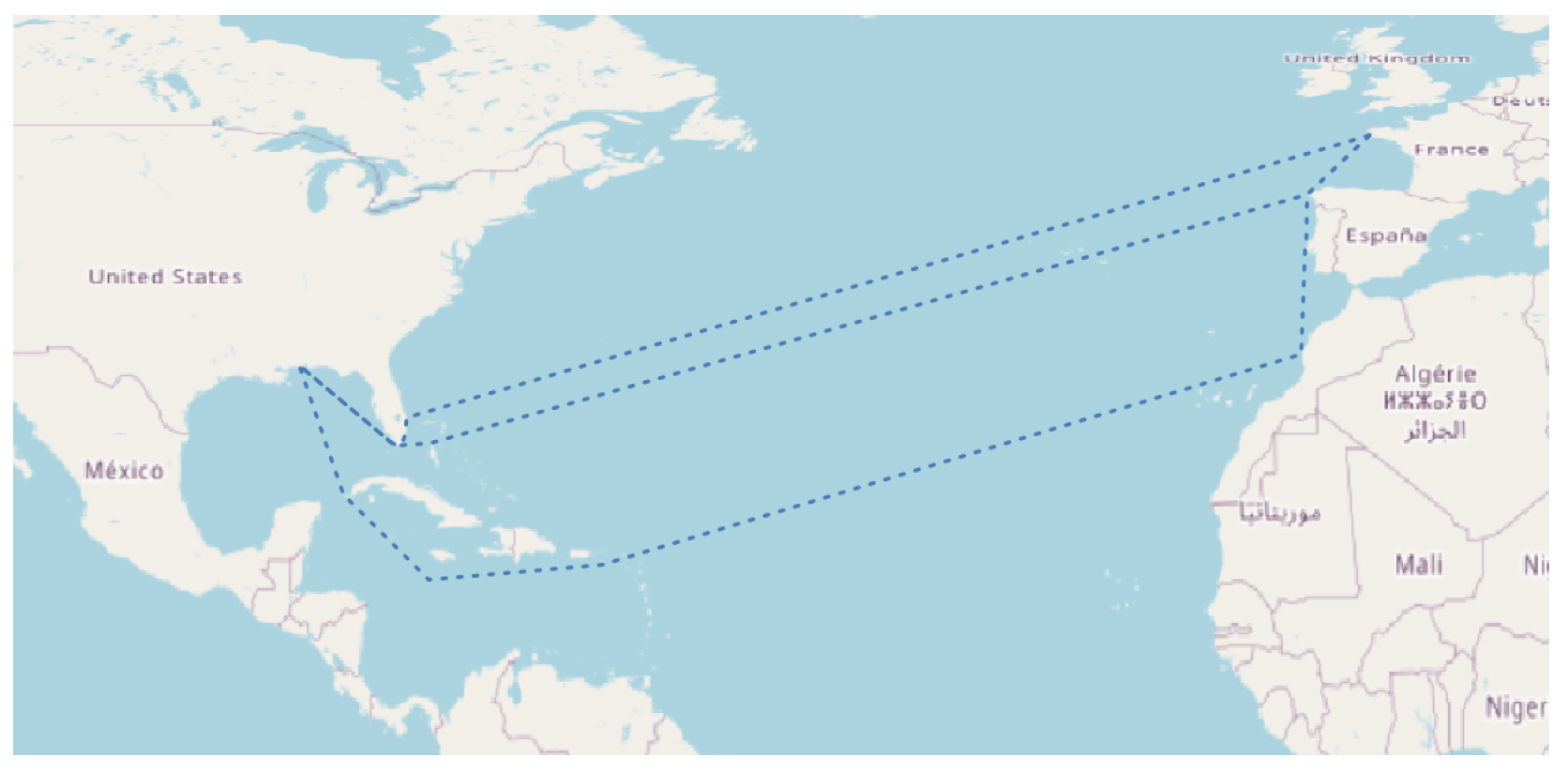
| Route | Savannah, U.S. to Algeciras, Spain |
| Length between perpendiculars (m) | 175 |
| Beam (m) | 25.4 |
| Average Draft (m) | 9.5 |
| Design Speed (knot) | 20 |
| Displacement (m3) | 24,053 |
| Block Coef | 0.561 |
| Prismatic coefficient | 0.589 |
| Position of LCG (m) | 86.5 |
| Fuel Type | HFO |
| Engine | 6S60ME |
| Engine MCR @ L1 (kWh) | 14,940 |
| Engine RPM @ L1 | 105 |
| Engine Eff at L1 | 0.5018 |
| Propeller Diam (m) | 5.0 |
| Propeller Pitch (m) | 4.75 |
| Propeller Blade Count | 5 |
| Propeller Expanded Area Ratio | 0.8 |
| Weight (ton) | 24,610.0 |
| Date | HFO Consumption (tons) |
|---|---|
| Nov. 2023 | 478.22 |
| Dec. 2023 | 471.06 |
| Jan. 2024 | 482.85 |
| Feb. 2024 | 463.68 |
| Mar. 2024 | 480.17 |
| Apr. 2024 | 483.70 |
| May 2024 | 478.07 |
| Jun. 2024 | 468.89 |
| Jul. 2024 | 466.27 |
| Aug. 2024 | 468.15 |
| Sep. 2024 | 464.79 |
| Oct. 2024 | 473.03 |
| Ideal Conditions | 456.42 |
Disclaimer/Publisher’s Note: The statements, opinions and data contained in all publications are solely those of the individual author(s) and contributor(s) and not of MDPI and/or the editor(s). MDPI and/or the editor(s) disclaim responsibility for any injury to people or property resulting from any ideas, methods, instructions or products referred to in the content. |
© 2025 by the authors. Licensee MDPI, Basel, Switzerland. This article is an open access article distributed under the terms and conditions of the Creative Commons Attribution (CC BY) license (https://creativecommons.org/licenses/by/4.0/).
Share and Cite
Aredah, A.; Rakha, H.A. ShipNetSim: An Open-Source Simulator for Real-Time Energy Consumption and Emission Analysis in Large-Scale Maritime Networks. J. Mar. Sci. Eng. 2025, 13, 518. https://doi.org/10.3390/jmse13030518
Aredah A, Rakha HA. ShipNetSim: An Open-Source Simulator for Real-Time Energy Consumption and Emission Analysis in Large-Scale Maritime Networks. Journal of Marine Science and Engineering. 2025; 13(3):518. https://doi.org/10.3390/jmse13030518
Chicago/Turabian StyleAredah, Ahmed, and Hesham A. Rakha. 2025. "ShipNetSim: An Open-Source Simulator for Real-Time Energy Consumption and Emission Analysis in Large-Scale Maritime Networks" Journal of Marine Science and Engineering 13, no. 3: 518. https://doi.org/10.3390/jmse13030518
APA StyleAredah, A., & Rakha, H. A. (2025). ShipNetSim: An Open-Source Simulator for Real-Time Energy Consumption and Emission Analysis in Large-Scale Maritime Networks. Journal of Marine Science and Engineering, 13(3), 518. https://doi.org/10.3390/jmse13030518