

Enhanced Seafloor Topography Inversion Using an Attention Channel 1D Convolutional Network Based on Multiparameter Gravity Data: Case Study of the Mariana Trench
 ,
,  , , , , , , and
Abstract
1. Introduction
2. Material and Methods
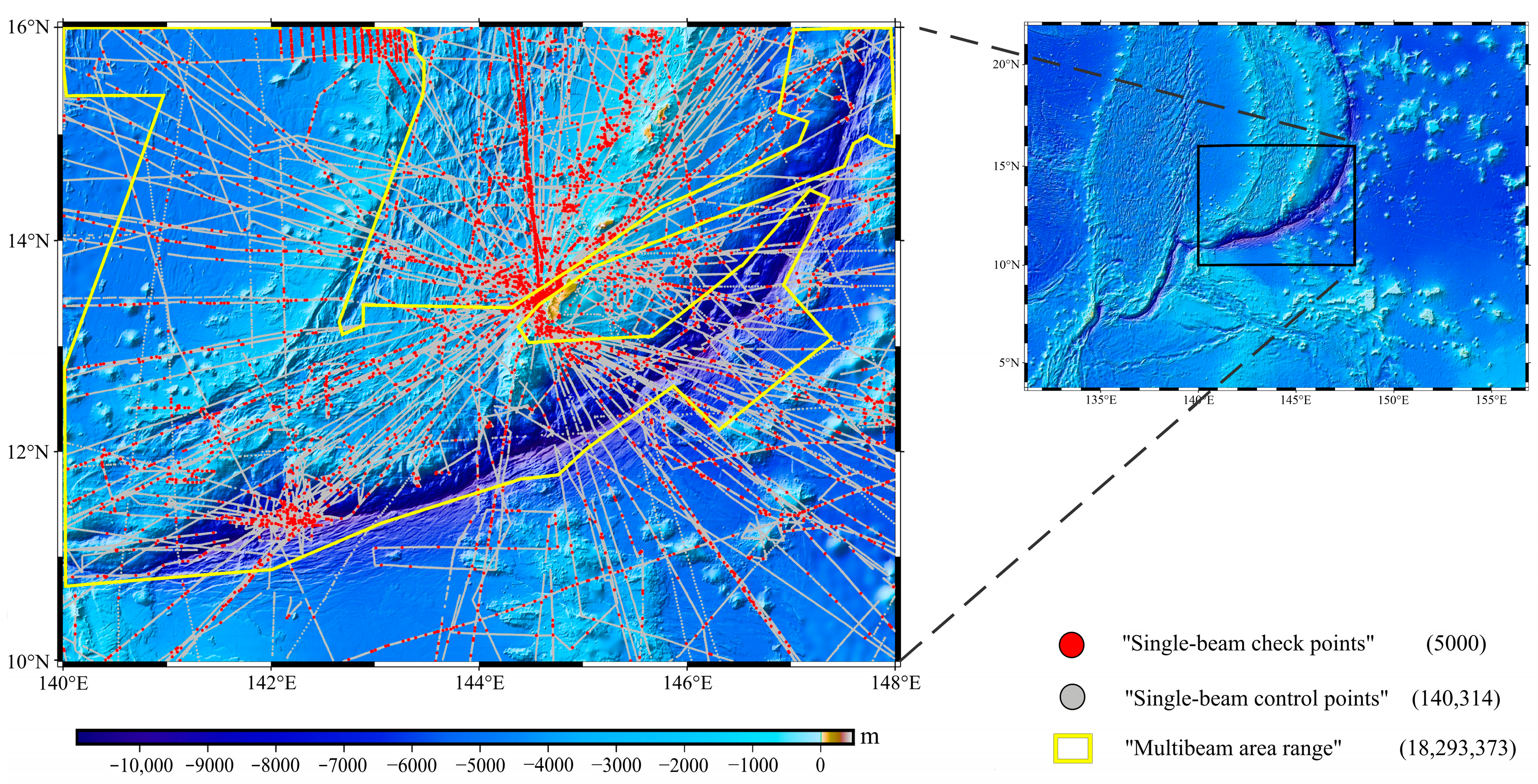
2.1. Study Area
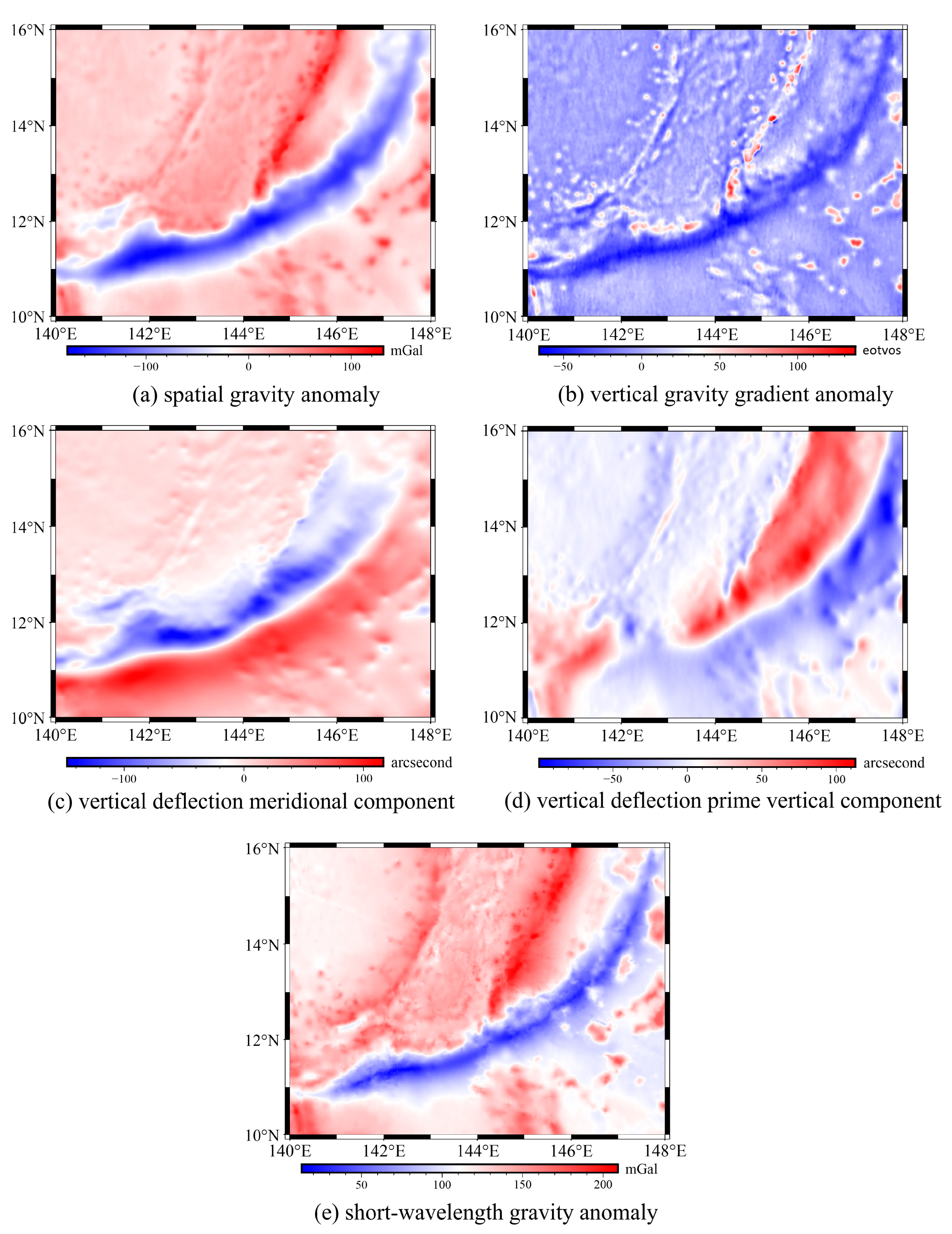
2.2. Data
2.3. Methodology
2.3.1. Data Preprocessing
2.3.2. Methodology
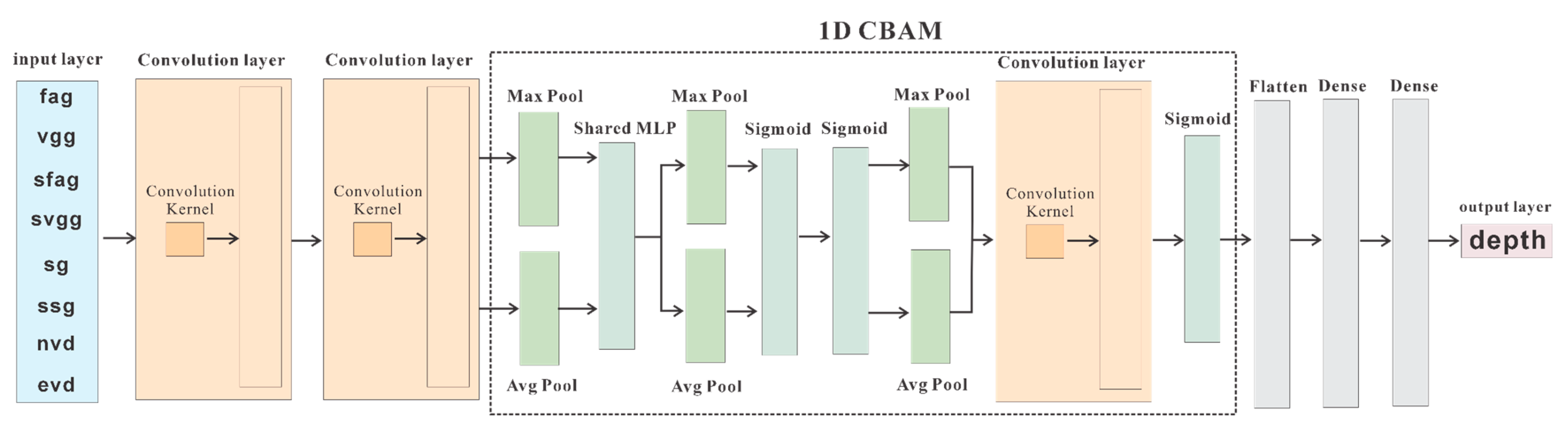
AC1D
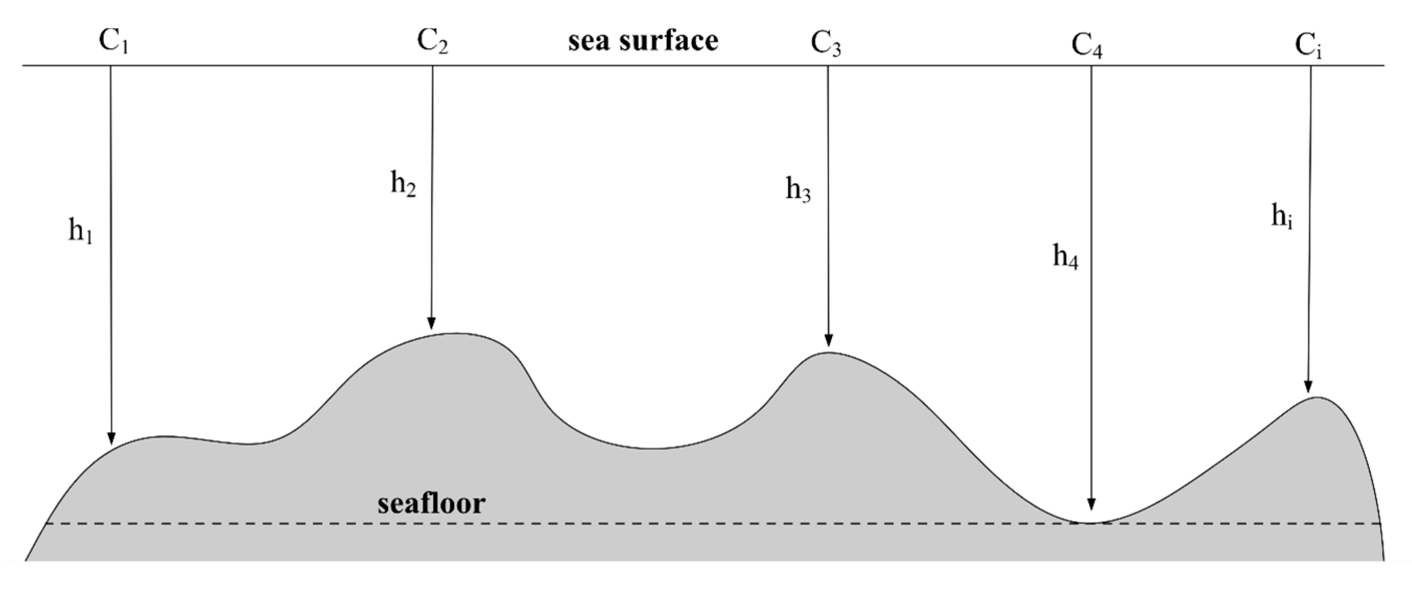
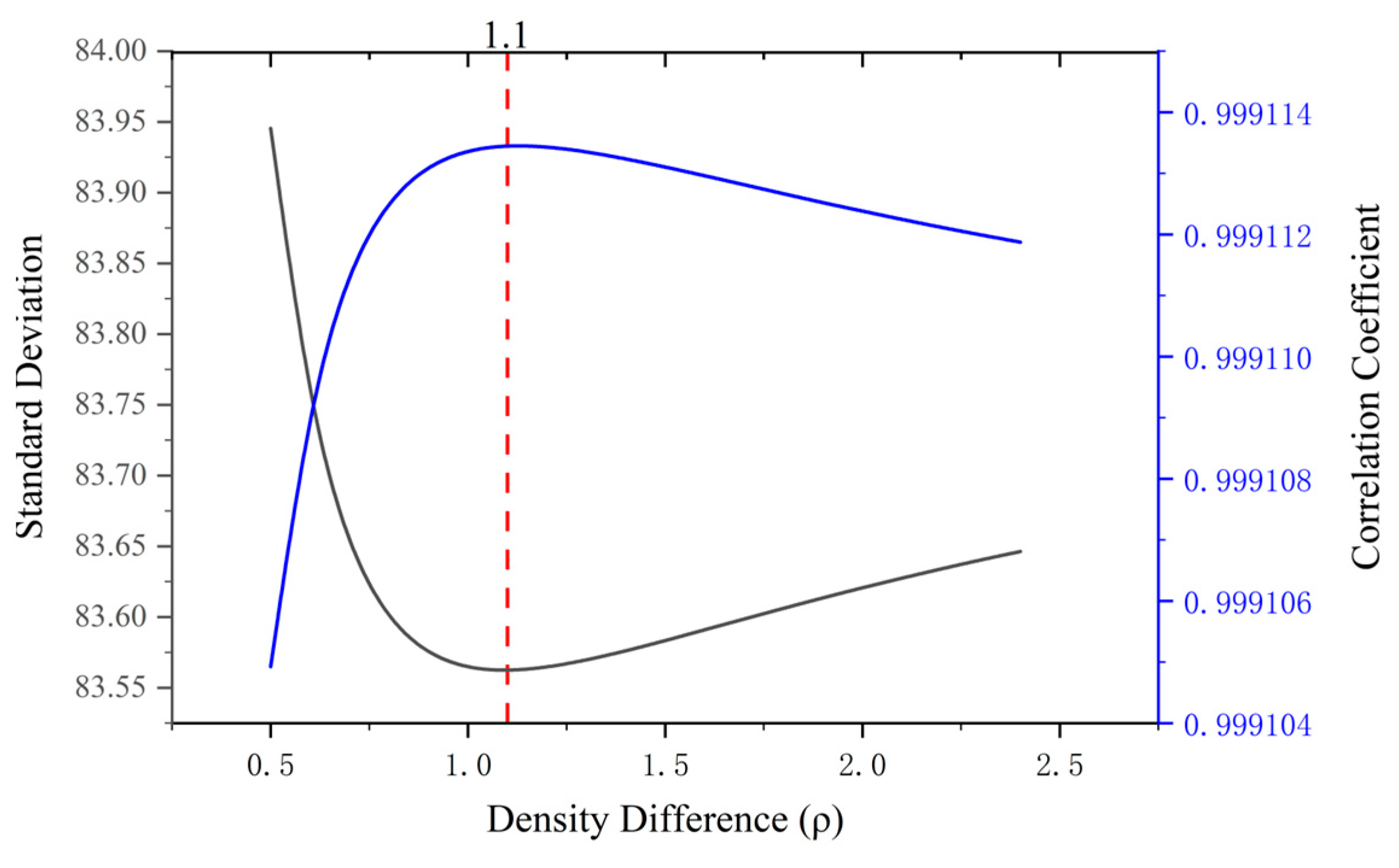
GGM
PLBP
CNN
2.3.3. Environment and Runtime
2.3.4. Evaluation Metrics
3. Results and Evaluation
3.1. AC1D Bathymetric Grid Results
3.2. Validation with Single-Beam Data
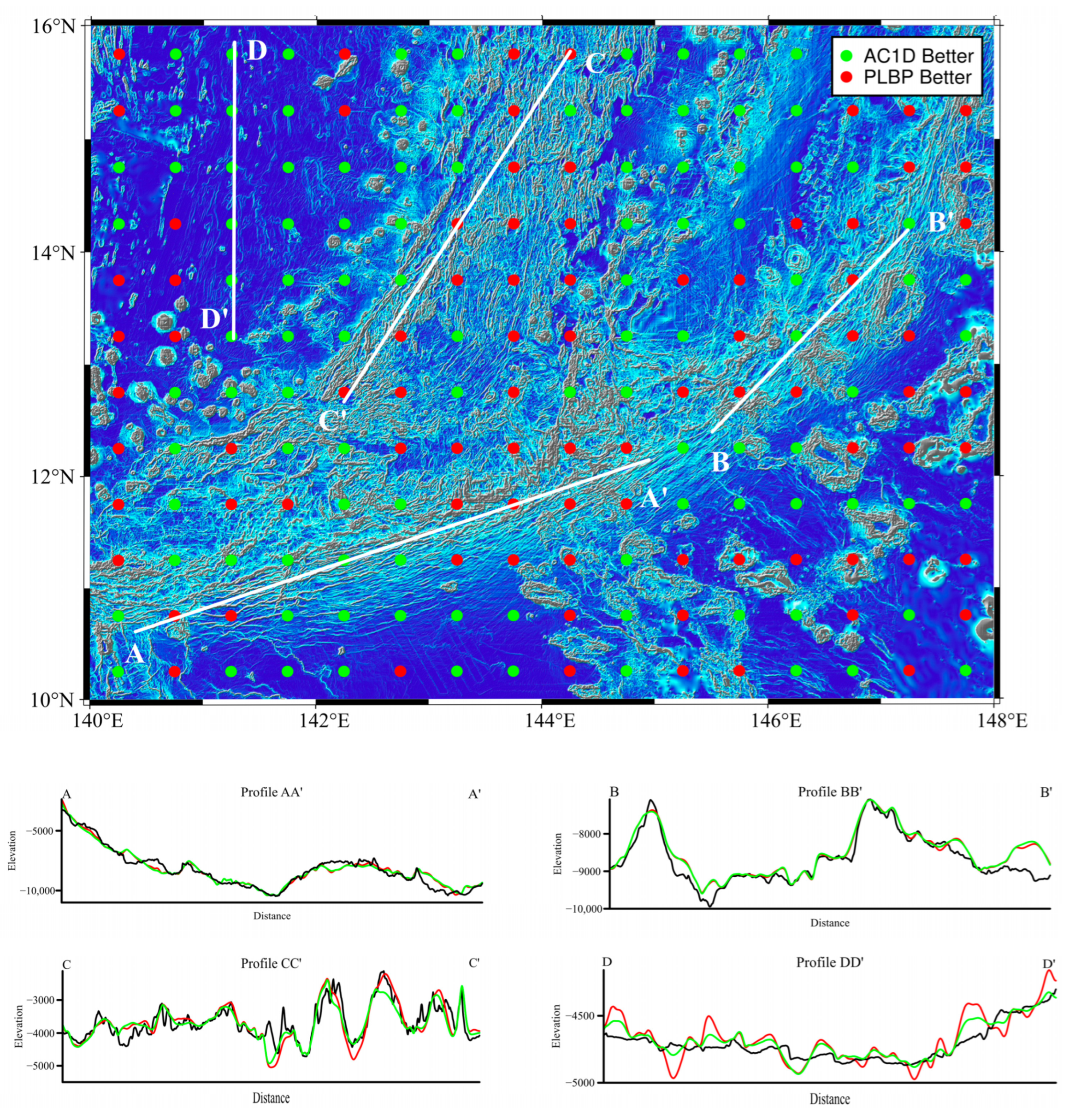
3.3. Validation with Multibeam Data
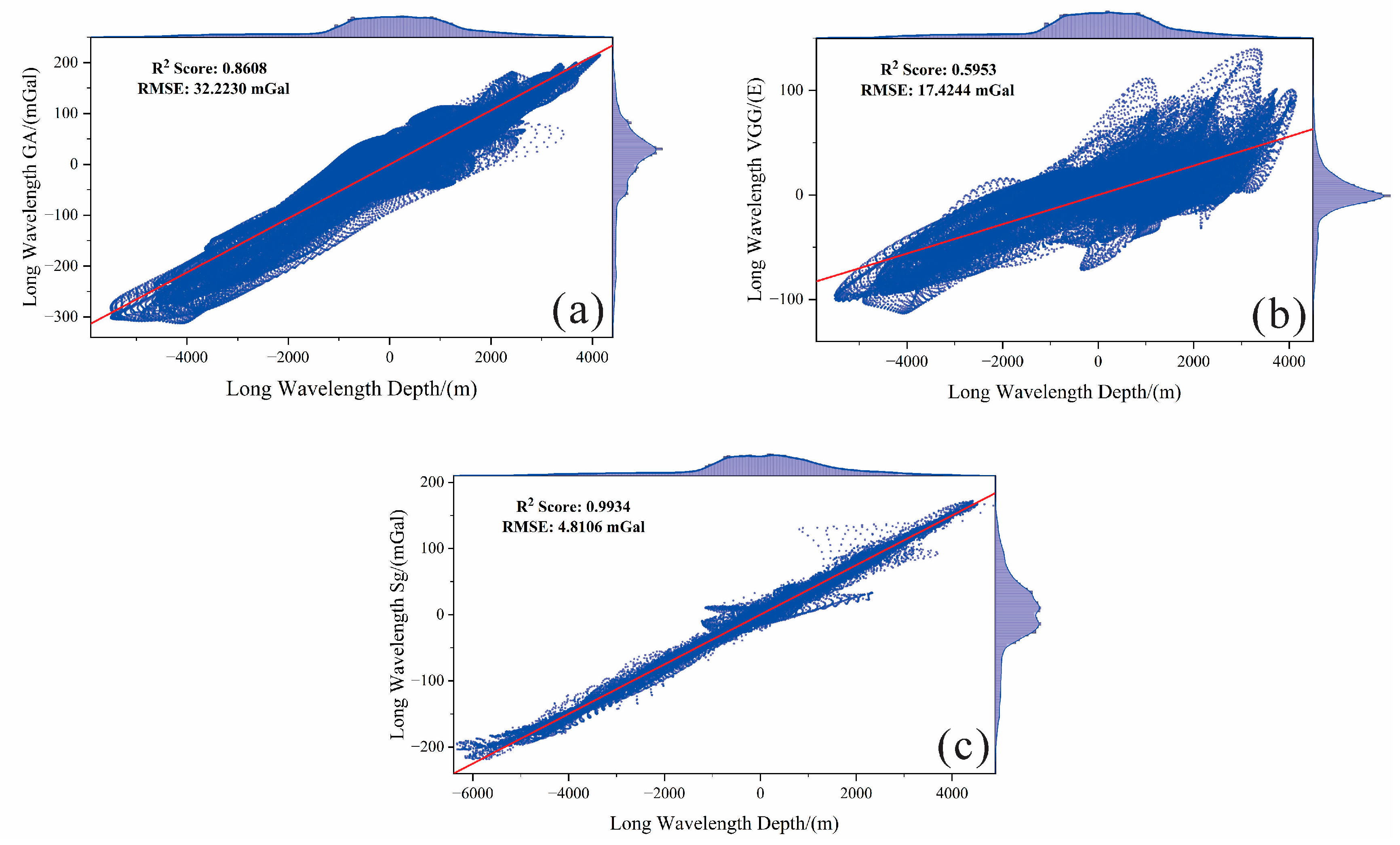
3.4. Correlation Analysis with GEBCO2023
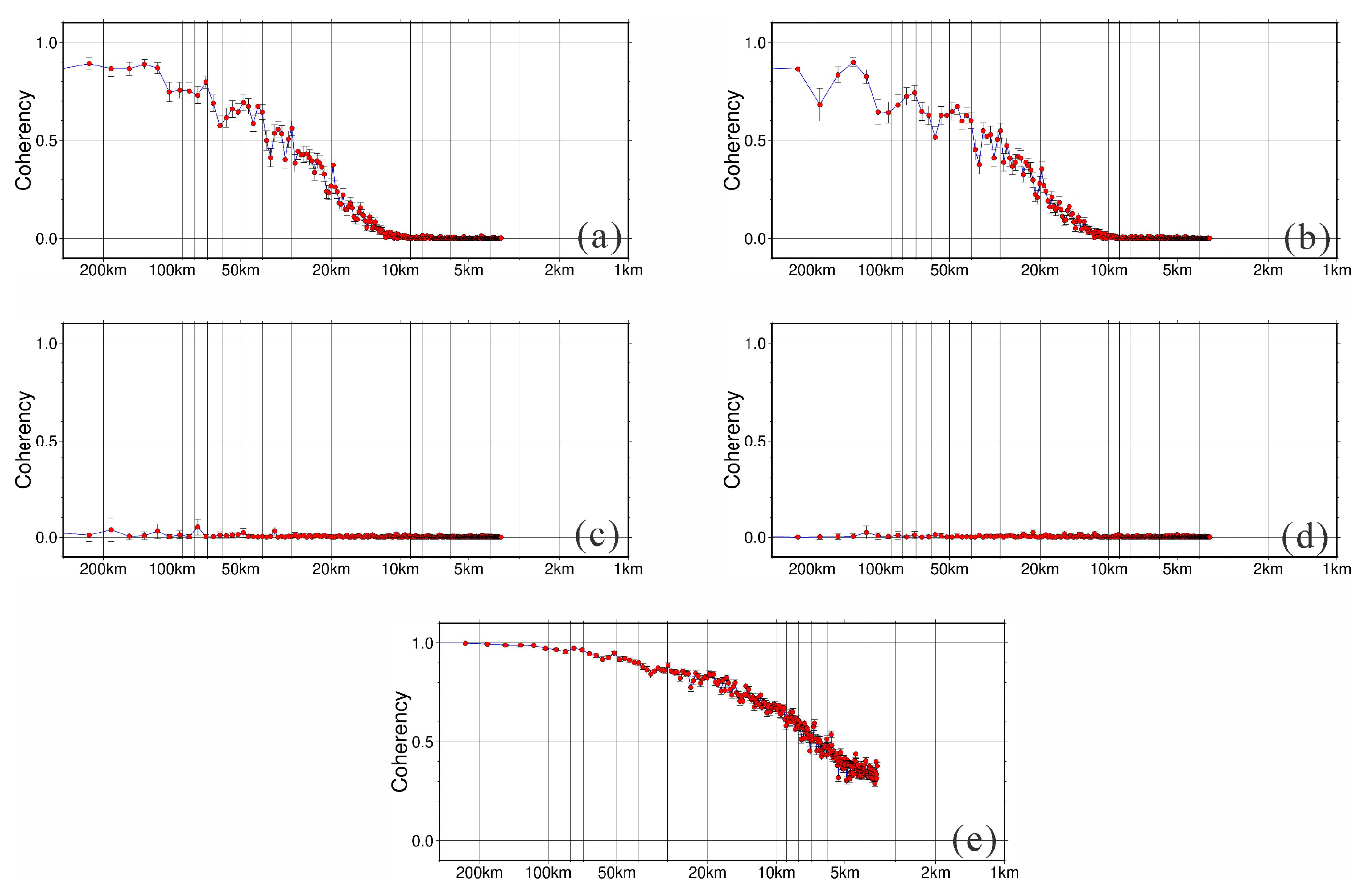
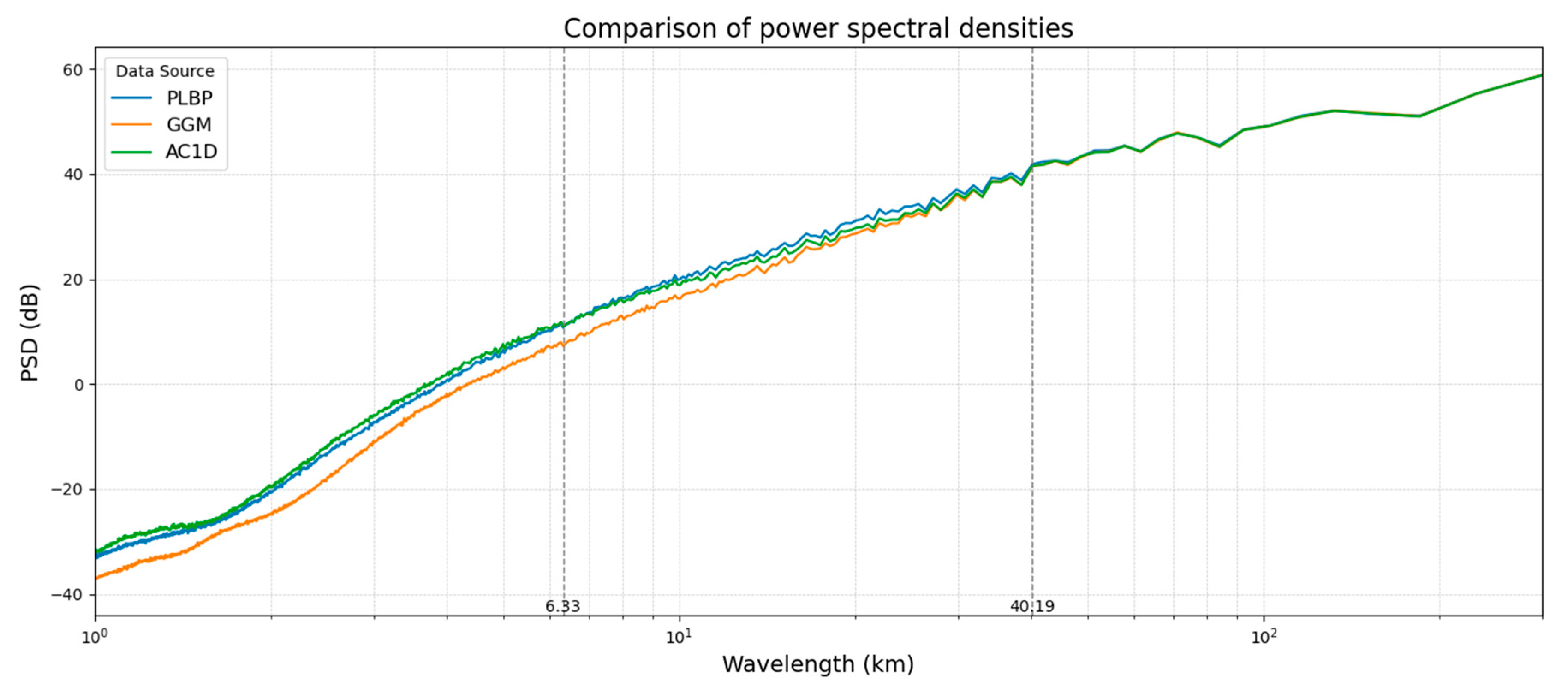
3.5. Power Spectral Density Evaluation
4. Conclusions
Author Contributions
Funding
Institutional Review Board Statement
Informed Consent Statement
Data Availability Statement
Acknowledgments
Conflicts of Interest
References
- Wu, Z.; Yang, F.; Tang, Y. High-Resolution Seafloor Survey and Applications; Science Press: Beijing, China, 2021. [Google Scholar] [CrossRef]
- Sandwell, D.T.; Goff, J.A.; Gevorgian, J.; Harper, H.; Kim, S.-S.; Yu, Y.; Tozer, B.; Wessel, P.; Smith, W.H.F. Improved Bathymetric Prediction Using Geological Information: SYNBATH. Earth Space Sci. 2022, 9, e2021EA002069. [Google Scholar] [CrossRef]
- Smith, W.H.; Sandwell, D.T. Bathymetric prediction from dense satellite altimetry and sparse shipboard bathymetry. J. Geophys. Res. 1994, 99, 21803–21824. [Google Scholar] [CrossRef]
- Hu, M.; Li, L.; Jin, T.; Jiang, W.; Wen, H.; Li, J. A New 1′ × 1′ Global Seafloor Topography Model Predicted from Satellite Altimetric Vertical Gravity Gradient Anomaly and Ship Soundings BAT_VGG2021. Remote Sens. 2021, 13, 3515. [Google Scholar] [CrossRef]
- Harper, H.; Sandwell, D.T. Global predicted bathymetry using neural networks. Earth Space Sci. 2024, 11, e2023EA003199. [Google Scholar] [CrossRef]
- Zhou, S.; Guo, J.; Zhang, H.; Jia, Y.; Sun, H.; Liu, X.; An, D. SDUST2023BCO: A global seafloor model determined from a multi-Layer perceptron neural network using multi-source differential marine geodetic data. Earth Syst. Sci. Data 2025, 17, 165–179. [Google Scholar] [CrossRef]
- Mayer, L.; Jakobsson, M.; Allen, G.; Dorschel, B.; Falconer, R.; Ferrini, V.; Lamarche, G.; Snaith, H.; Weatherall, P. The nippon foundation—GEBCO seabed 2030 project: The quest to see the world’s oceans completely mapped by 2030. Geosciences 2018, 8, 63. [Google Scholar] [CrossRef]
- Zheng, Q.; Chen, S. Review on the recent developments of terrestrial water storage variations using GRACE satellite-based Datum. Prog. Geophys. 2015, 30, 2603–2615. [Google Scholar] [CrossRef]
- Han, T.; Zhang, H.; Cao, W.; Le, C.; Wang, C.; Yang, X.; Ma, Y.; Li, D.; Wang, J.; Lou, X. Cost-efficient bathymetric mapping method based on massive active–passive remote sensing data. ISPRS J. Photogramm. Remote Sens. 2023, 203, 285–300. [Google Scholar] [CrossRef]
- Guan, J.; Zhang, H.; Han, T.; Cao, W.; Wang, J.; Li, D. High-resolution mapping of shallow water bathymetry based on the scale-invariant effect using Sentinel-2 and GF-1 satellite remote sensing data. Remote Sens. 2025, 17, 640. [Google Scholar] [CrossRef]
- Duan, Z.; Cheng, L.; Mao, Q.; Song, Y.; Zhou, X.; Li, M.; Gong, J. MIWC: A Multi-temporal image weighted composition method for satellite-derived bathymetry in shallow waters. ISPRS J. Photogramm. Remote Sens. 2024, 218, 430–445. [Google Scholar] [CrossRef]
- Qin, X.; Wu, Z.; Luo, X.; Shang, J.; Zhao, D.; Zhou, J.; Cui, J.; Wan, H.; Xu, G. MuSRFM: Multiple scale resolution fusion based precise and robust satellite derived bathymetry model for island nearshore shallow water regions using Sentinel-2 multi-spectral imagery. ISPRS J. Photogramm. Remote Sens. 2024, 218, 150–169. [Google Scholar] [CrossRef]
- Klokočník, J.; Kostelecký, J.; Bezděk, A. Gravity strike angles from EIGEN6C4 to seek conditions favourable for hydrocarbon occurrences in the Arctic zone. Polar Sci. 2024, 101157. [Google Scholar] [CrossRef]
- Eppelbaum, L.; Katz, Y.; Klokočník, J.; Kostelecký, J.; Zheludev, V.; Ben-Avraham, Z. Tectonic insights into the Arabian-African region inferred from a comprehensive examination of satellite gravity big data. Glob. Planet. Change 2018, 171, 65–87. [Google Scholar] [CrossRef]
- Kim, J.W.; von Frese, R.R.B.; Lee, B.Y.; Roman, D.R.; Doh, S.-J. Altimetry-derived gravity predictions of bathymetry by the gravity-geologic method. Pure Appl. Geophys. 2011, 168, 815–826. [Google Scholar] [CrossRef]
- Wei, Z.; Guo, J.; Zhu, C.; Yuan, J.; Chang, X.; Ji, B. Evaluating Accuracy of HY-2A/GM-Derived Gravity Data with the Gravity-Geologic Method to Predict Bathymetry. Front. Earth Sci. 2021, 9, 636246. [Google Scholar] [CrossRef]
- Hsiao, Y.-S.; Hwang, C.; Cheng, Y.-S.; Chen, L.-C.; Hsu, H.-J.; Tsai, J.-H.; Liu, C.-L.; Wang, C.-C.; Liu, Y.-C.; Kao, Y.-C. High-resolution depth and coastline over major atolls of South China Sea from satellite altimetry and imagery. Remote Sens. Environ. 2016, 176, 69–83. [Google Scholar] [CrossRef]
- An, D.; Guo, J.; Li, Z.; Ji, B.; Liu, X.; Chang, X. Improved Gravity-Geologic Method Reliably Removing the Long-Wavelength Gravity Effect of Regional Seafloor Topography: A Case of Bathymetric Prediction in the South China Sea. IEEE Trans. Geosci. Remote Sens. 2022, 60, 4211912. [Google Scholar] [CrossRef]
- McKenzie, D.P.; Bowin, C. The relationship between bathymetry and gravity in the Atlantic Ocean. J. Geophys. Res. 1976, 81, 1903–1915. [Google Scholar] [CrossRef]
- Xu, C.; Li, J.; Jian, G.; Wu, Y.; Zhang, Y. An adaptive nonlinear iterative method for predicting seafloor topography from altimetry-derived gravity data. J. Geophys. Res. Solid Earth 2023, 128, e2022JB025692. [Google Scholar] [CrossRef]
- Smith, W.H.; Sandwell, D.T. Global Sea Floor Topography from Satellite Altimetry and Ship Depth Soundings. Science 1997, 277, 1956–1962. [Google Scholar] [CrossRef]
- Vergos, G.S.; Siders, M.G. Improvement in the determination of the marine geoid by estimating the bathymetry from altimetry and depth soundings. Mar. Geod. 2005, 28, 81–102. [Google Scholar] [CrossRef]
- Fan, D.; Li, S.; Li, X.; Yang, J.; Wan, X. Seafloor Topography Estimation from Gravity Anomaly and Vertical Gravity Gradient Using Nonlinear Iterative Least Square Method. Remote Sens. 2021, 13, 64. [Google Scholar] [CrossRef]
- Dorman, L.M.; Lewis, B.T.R. Experimental isostasy: 1. Theory of the determination of the earth’s isostatic response to a concentrated load. J. Geophys. Res. 1970, 75, 3357–3365. [Google Scholar] [CrossRef]
- Sandwell, D.T.; Smith, W.H.F. Marine gravity anomaly from Geosat and ERS 1 satellite altimetry. J. Geophys. Res. Solid Earth 1997, 102, 10039–10054. [Google Scholar] [CrossRef]
- Hu, M.; Li, J.; Jin, T.; Xu, X.; Xing, L.; Wu, Y. Recovery of bathymetry over China Sea and its adjacent areas by combination of multi-source data. Geomat. Inf. Wuhan Univ. 2015, 40, 1266–1273. (In Chinese) [Google Scholar] [CrossRef]
- Fan, D.; Li, S.; Yang, J.; Meng, S.; Xing, Z.; Zhang, C.; Feng, J. Predicting bathymetry by applying multiple regression analysis in the Southwest Indian Ocean Region. Acta Geod. Cartogr. Sin. 2020, 49, 147–161. (In Chinese) [Google Scholar] [CrossRef]
- Chen, X.; Zhong, M.; Sun, M.; An, D.; Feng, W.; Yang, M. Recovering bathymetry using BP neural network combined with modified gravity–geologic method: A case study in the South China Sea. Remote Sens. 2024, 16, 4023. [Google Scholar] [CrossRef]
- Harishidayat, D.; Al-Shuhail, A.; Randazzo, G.; Lanza, S.; Muzirafuti, A. Reconstruction of Land and Marine Features by Seismic and Surface Geomorphology Techniques. Appl. Sci. 2022, 12, 9611. [Google Scholar] [CrossRef]
- Ge, B.; Guo, J.; Kong, Q.; Zhu, C.; Huang, L.; Sun, H.; Liu, X. Seafloor topography inversion from multi-source marine gravity Data using multi-channel convolutional neural network. Eng. Appl. Artif. Intell. 2025, 139, 109567. [Google Scholar] [CrossRef]
- Sun, H.; Li, Q.; Bao, L.; Wu, Z.; Wu, L. Progress and development trend of global refined seafloor topography modeling. Geomat. Inf. Wuhan Univ. 2022, 47, 1555–1567. (In Chinese) [Google Scholar] [CrossRef]
- Annan, R.F.; Wan, X. Recovering Bathymetry of the Gulf of Guinea Using Altimetry-Derived Gravity Field Products Combined via Convolutional Neural Network. Surv. Geophys. 2022, 43, 1541–1561. [Google Scholar] [CrossRef]
- Yang, L.; Liu, M.; Liu, N.; Guo, J.; Lin, L.; Zhang, Y.; Du, X.; Xu, Y.; Zhu, C.; Wang, Y. Recovering Bathymetry from Satellite Altimetry-Derived Gravity by Fully Connected Deep Neural Network. IEEE Geosci. Remote Sens. Lett. 2023, 20, 1502805. [Google Scholar] [CrossRef]
- Li, Q.; Zhai, Z.; Li, Q.; Wu, L.; Bao, L.; Sun, H. Improved bathymetry in the South China Sea from multisource gravity field elements using fully connected neural network. J. Mar. Sci. Eng. 2023, 11, 1345. [Google Scholar] [CrossRef]
- Sun, H.; Feng, Y.; Fu, Y.; Sun, W.; Peng, C.; Zhou, X.; Zhou, D. Bathymetric Prediction Using Multisource Gravity Data Derived from a Parallel Linked BP Neural Network. J. Geophys. Res. Solid Earth 2022, 127, e2022JB024428. [Google Scholar] [CrossRef]
- Zhang, B.; Xiong, W.; Ma, M.; Wang, M.; Wang, D.; Huang, X.; Yu, L.; Zhang, Q.; Lu, H.; Hong, D.; et al. Super-Resolution Reconstruction of a 3 Arc-Second Global DEM Dataset. Sci. Bull. 2022, 67, 2526–2530. [Google Scholar] [CrossRef]
- Chen, X.; Luo, X.; Wu, Z.; Qin, X.; Shang, J.; Li, B.; Wang, M.; Wan, H. A VGGNet-based method for refined bathymetry from satellite altimetry to reduce errors. Remote Sens. 2022, 14, 5939. [Google Scholar] [CrossRef]
- Chen, X.; Luo, X.; Wu, Z.; Qin, X.; Shang, J.; Xu, H.; Li, B.; Wang, M.; Wan, H. A VGGNet-based correction for satellite altimetry-derived gravity anomalies to improve the accuracy of bathymetry to depths of 6500 m. Acta Oceanol. Sin. 2024, 43, 112–122. [Google Scholar] [CrossRef]
- Alzubaidi, L.; Zhang, J.; Humaidi, A.J.; Al-Dujaili, A.; Duan, Y.; Al-Shamma, O.; Santamaría, J.; Fadhel, M.A.; Al-Amidie, M.; Farhan, L. Review of deep learning: Concepts, CNN architectures, challenges, applications, future directions. J. Big Data 2021, 8, 83. [Google Scholar] [CrossRef]
- Huang, S.; Tang, J.; Dai, J.; Wang, Y. Signal Status Recognition Based on 1DCNN and Its Feature Extraction Mechanism Analysis. Sensors 2019, 19, 2018. [Google Scholar] [CrossRef]
- Zhou, Z.; Lin, J.; Behn, M.D.; Olive, J.-A. Mechanism for Normal Faulting in the Subducting Plate at the Mariana Trench. Geophys. Res. Lett. 2015, 42, 4309–4317. [Google Scholar] [CrossRef]
- Fryer, P.; Becker, N.; Appelgate, B.; Martinez, F.; Edwards, M.; Fryer, G. Why Is the Challenger Deep so Deep? Earth Planet. Sci. Lett. 2003, 211, 259–269. [Google Scholar] [CrossRef]
- Fujioka, K.; Okino, K.; Kanamatsu, T.; Ohara, Y. Morphology and Origin of the Challenger Deep in the Southern Mariana Trench. Geophys. Res. Lett. 2002, 29, 1372. [Google Scholar] [CrossRef]
- Lemenkova, P. Statistical Analysis of the Mariana Trench Geomorphology Using R Programming Language. Geod. Cartogr. 2019, 45, 57–84. [Google Scholar] [CrossRef]
- Liu, Y.; Wu, Z.; Le Pourhiet, L.; Coltice, N.; Li, C.-F.; Shang, J.; Zhao, D.; Zhou, J.; Wang, M. Geomorphology and Mechanisms of Subduction Erosion in the Sediment-Starved Mariana Convergent Margin. Geomorphology 2024, 454, 109161. [Google Scholar] [CrossRef]
- Bolón-Canedo, V.; Sánchez-Maroño, N.; Alonso-Betanzos, A. Feature Selection for High-Dimensional Data. Prog. Artif. Intell. 2016, 5, 65–75. [Google Scholar] [CrossRef]
- Wessel, P.; Luis, J.F.; Uieda, L.; Scharroo, R.; Wobbe, F.; Smith, W.H.F.; Tian, D. The Generic Mapping Tools Version 6. Geochem. Geophys. Geosyst. 2019, 20, 5556–5564. [Google Scholar] [CrossRef]
- Zheng, A.; Casari, A. Feature Engineering for Machine Learning: Principles and Techniques for Data Scientists; O’Reilly Media, Inc.: Sebastopol, CA, USA, 2018; ISBN 978-1-4919-5319-8. [Google Scholar]
- Khalid, S.; Khalil, T.; Nasreen, S. A Survey of Feature Selection and Feature Extraction Techniques in Machine Learning. In Proceedings of the 2014 Science and Information Conference, London, UK, 27–29 August 2014; IEEE: Piscataway, NJ, USA, 2014; pp. 372–378. [Google Scholar]
- Parker, R.L. The Rapid Calculation of Potential Anomalies. Geophys. J. Roy. Astron. Soc. 1973, 31, 447–455. [Google Scholar] [CrossRef]
- Watts, A.B. An Analysis of Isostasy in the World’s Oceans 1. Hawaiian-Emperor Seamount Chain. J. Geophys. Res. Solid Earth 1978, 83, 5989–6004. [Google Scholar] [CrossRef]
- Wold, S.; Esbensen, K.; Geladi, P. Principal Component Analysis. Chemom. Intell. Lab. Syst. 1987, 2, 37–52. [Google Scholar] [CrossRef]
- Woo, S.; Park, J.; Lee, J.-Y.; Kweon, I.S. Cbam: Convolutional block attention module. In Proceedings of the European Conference on Computer Vision (ECCV), Munich, Germany, 8–14 September 2018; pp. 3–19. [Google Scholar]
- Ibrahim, A.; Hinze, W.J. Mapping Buried Bedrock Topography with Gravity. Ground Water 1972, 10, 18–23. [Google Scholar] [CrossRef]
- Hsiao, Y.-S.; Kim, J.W.; Kim, K.B.; Lee, B.Y.; Hwang, C. Bathymetry Estimation Using the Gravity-Geologic Method: An Investigation of Density Contrast Predicted by the Downward Continuation Method. Terr. Atmos. Ocean Sci. 2011, 22, 347. [Google Scholar] [CrossRef]
- Hu, M.Z.; Li, J.C.; Jin, T.Y. Bathymetry Inversion with Gravity-Geologic Method in Emperor Seamount. Geomat. Inf. Wuhan Univ. 2012, 37, 610–612. (In Chinese) [Google Scholar] [CrossRef]
- Kim, K.B.; Yun, H.S. Satellite-derived bathymetry prediction in shallow waters using the gravity-geologic method: A Case Study in the West Sea of Korea. KSCE J. Civ. Eng. 2018, 22, 2560–2568. [Google Scholar] [CrossRef]


| Operating System | CPU | CPU Memory | GPU | GPU Memory |
|---|---|---|---|---|
| Windows 11 | Intel(R) Core(TM) i5-13400F CPU @ 2.50 GHz (Inter, Santa Clara, CA, USA) | 32 GB | NVIDIA GeForce RTX 4070 Ti | 12 GB |
| Metrics | Formula | Symbol Definitions | Formula Functionality |
|---|---|---|---|
| STD | : the number of data points : the data point in the dataset : the mean of the dataset | Measures dataset dispersion; indicates average deviation from the mean. Larger values imply more dispersion. | |
| RMSE | : the i-th actual observation : the i-th predicted value | A common regression error metric assesses the difference between predictions and observations, which reflects average deviation. Lower RMSE indicates better model performance. | |
| MRE | : the i-th actual observation : the i-th predicted value | Represents the average relative error between predictions and actual values; measures the model’s average relative error. Smaller MRE indicates better model fit. | |
| MAE | : the i-th actual observation : the i-th predicted value | A common regression error metric measuring the average error between predictions and actual values. Unlike RMSE, MAE is less sensitive to large errors, providing a more straightforward average deviation. Lower MAE indicates better model performance. | |
| R | : the data point in the dataset X : the mean of the dataset X : the data point in the dataset Y : the mean of the dataset Y | A statistical metric for measuring the linear relationship between two variables, ranging from −1 to 1, indicating the strength and direction of correlation. When R is between 0.7 and 1, it indicates a strong positive correlation. |
| Method | Input Parameters | STD (m) | RMSE (m) |
|---|---|---|---|
| GGM | fag | 71.61 | 88.20 |
| PLBP | fag vgg sfag svgg | 60.52 | 73.27 |
| AC1D | fag vgg sfag svgg sg ssg nvd evd | 56.70 | 68.06 |
| CNN | lon lat fag vgg sg nvd evd | 89.69 | 138.97 |
| GEBCO2023 | 92.91 | 109.07 |
| Grid | Max (m) | Min (m) | STD (m) | RMSE (m) | MAE (m) | MRE (%) | R |
|---|---|---|---|---|---|---|---|
| PLBP | 2294.34 | −1545.72 | 177.80 | 234.61 | 153.07 | 4.14 | 0.98752 |
| AC1D | 2212.85 | −1561.99 | 161.75 | 210.82 | 135.21 | 3.59 | 0.98981 |
| SAC1D | 2387.17 | −1556.26 | 161.67 | 211.59 | 136.51 | 3.63 | 0.98974 |
| AC1D4 | 2301.55 | −1476.59 | 176.01 | 226.50 | 142.55 | 3.81 | 0.98825 |
| GEBCO2023 | 1184.55 | −803.71 | 37.76 | 37.77 | 20.88 | 0.56 | 0.9997 |
| Grid | RMSE (m) | STD (m) | MAE (m) | R |
|---|---|---|---|---|
| AC1D Better Area | ||||
| AC1D | 161.28 | 116.00 | 111.25 | 0.8955 |
| PLBP | 205.44 | 148.21 | 140.98 | 0.8615 |
| PLBP Better Area | ||||
| AC1D | 238.46 | 170.33 | 165.45 | 0.8755 |
| PLBP | 222.62 | 156.15 | 157.59 | 0.8961 |
| ALL Area | ||||
| AC1D | 189.40 | 134.40 | 132.49 | 0.8958 |
| PLBP | 220.58 | 158.35 | 152.20 | 0.8679 |
Disclaimer/Publisher’s Note: The statements, opinions and data contained in all publications are solely those of the individual author(s) and contributor(s) and not of MDPI and/or the editor(s). MDPI and/or the editor(s) disclaim responsibility for any injury to people or property resulting from any ideas, methods, instructions or products referred to in the content. |
© 2025 by the authors. Licensee MDPI, Basel, Switzerland. This article is an open access article distributed under the terms and conditions of the Creative Commons Attribution (CC BY) license (https://creativecommons.org/licenses/by/4.0/).
Share and Cite
Wang, Q.; Wu, Z.; Wu, Z.; Wang, M.; Zhao, D.; Jin, T.; Zhao, Q.; Qin, X.; Liu, Y.; Jiang, Y.; et al. Enhanced Seafloor Topography Inversion Using an Attention Channel 1D Convolutional Network Based on Multiparameter Gravity Data: Case Study of the Mariana Trench. J. Mar. Sci. Eng. 2025, 13, 507. https://doi.org/10.3390/jmse13030507
Wang Q, Wu Z, Wu Z, Wang M, Zhao D, Jin T, Zhao Q, Qin X, Liu Y, Jiang Y, et al. Enhanced Seafloor Topography Inversion Using an Attention Channel 1D Convolutional Network Based on Multiparameter Gravity Data: Case Study of the Mariana Trench. Journal of Marine Science and Engineering. 2025; 13(3):507. https://doi.org/10.3390/jmse13030507
Chicago/Turabian StyleWang, Qiang, Ziyin Wu, Zhaocai Wu, Mingwei Wang, Dineng Zhao, Taoyong Jin, Qile Zhao, Xiaoming Qin, Yang Liu, Yifan Jiang, and et al. 2025. "Enhanced Seafloor Topography Inversion Using an Attention Channel 1D Convolutional Network Based on Multiparameter Gravity Data: Case Study of the Mariana Trench" Journal of Marine Science and Engineering 13, no. 3: 507. https://doi.org/10.3390/jmse13030507
APA StyleWang, Q., Wu, Z., Wu, Z., Wang, M., Zhao, D., Jin, T., Zhao, Q., Qin, X., Liu, Y., Jiang, Y., Zhao, P., & Zhang, N. (2025). Enhanced Seafloor Topography Inversion Using an Attention Channel 1D Convolutional Network Based on Multiparameter Gravity Data: Case Study of the Mariana Trench. Journal of Marine Science and Engineering, 13(3), 507. https://doi.org/10.3390/jmse13030507