Abstract
Accurately fitting bimodal wave spectra is crucial for understanding complex ocean conditions and promoting ocean-related research. In this context, this paper aims to solve the problem of reconstructing bimodal wave spectra in domestic island and reef areas. Taking measured data from the Jiangsu Xiangshui station in August 2017 and the Xisha Sea area on 1–3 August 2014 as case studies, the researchers selected three types of original bimodal wave spectra. After obtaining the sample spectra through fast Fourier transform and wave spectrum non-dimensionalization, this paper selected a novel wave spectrum—the rational fractional unimodal spectrum—and two classical wave spectra—the Jonswap spectrum and the Neumann spectrum. Three bimodal wave spectra were constructed by superimposing the low-frequency sub-spectrum and the high-frequency sub-spectrum. After using the improved PSO algorithm to optimize the parameters of these three bimodal wave spectra, the specific parameters were obtained. Comparisons were made between the above three bimodal wave spectra and three high-precision double-peak fitting spectra, the Huang Peiji six-parameter spectrum, the Ochi-Hubble spectrum, and the Shen Zhichun fitting spectrum, and the fitting effects were analyzed. The results demonstrated that when fitting the bimodal spectrum dominated by wind waves and the bimodal spectrum with comparable wind and swell energy, the combination of the rational fractional unimodal spectrum and the Neumann spectrum can achieve a fitting accuracy of up to 99%. When fitting the bimodal spectrum dominated by swell waves, the combination of the rational fractional unimodal spectrum and the Jonswap spectrum can also achieve a fitting accuracy of 99%. The findings of this paper provide valuable references for the study of other types of double-peak wave spectra in China.
1. Introduction
In the field of ocean observation, waves, a key and complex hydrographic phenomenon, occupy a central position in physical oceanography research and are an indispensable and critical input element in many fields such as ocean engineering, weather forecasting, and navigational safety. In view of the typical stochastic motion characteristics of ocean waves, spectral analysis has become a core technique to gain insight into such stochastic fluctuations.
As an important global strategic corridor and a national strategic priority for China, marine scientific research in the South China Sea is of great significance to national security and development. In the South China Sea, there are many islands and reefs, which are situated on the seabed on isolated terraces, surrounded by islands, sandbars, reefs, and shoals. The unique topography of the islands and reefs results in a variety of wave forms, among which bimodal waves are the most common. By fitting the bimodal spectrum, the complex sea conditions in the South China Sea can be more accurately described, providing key data support for marine engineering, helping the accurate design of ports and coastal projects, optimizing the foundation of offshore energy facilities, and improving the safety and durability of facilities. In the field of marine engineering and navigation, this can provide a reliable basis for the study of ship stability and assist in the planning of navigation routes to ensure the safety of navigation. At the level of marine scientific research, it can help accurately reveal the generation mechanisms and propagation laws of waves, quantify their impact on marine ecosystems, promote the continuous development of wave theory and nearshore engineering, and build a solid foundation for the all-round development of China’s marine industry.
The Neumann spectrum [1], Jonswap spectrum [2], and P–M spectrum [3] are widely used but mainly applicable to deep-water open-ocean conditions. Ochi and Hubble [4] derived a wave spectrum with six parameters through the superposition of two single-peaked wave spectra by integrating measured data in the North Atlantic. Torsethaugen [5,6] presented the Torsethaugen double-peak spectrum based on the Jonswap spectrum, combined with Norwegian measured data. Akbari et al. [7] analyzed measured data from the Gulf of Oman and used Jonswap spectra to represent wind waves and swell waves separately and then superimposed them to describe the double-peak spectrum. Winston G.G. [8] analyzed U.S. national ocean data to simulate single-peak spectra, using Jonswap and P–M spectra, and double-peak spectra, using the Torsethaugen spectrum, which improved accuracy when estimating wave spectra using the independent components of wind and swell. Rossi G.B. et al. [9] investigated the main parameters of the double-peak wave spectrum obtained by simulating the superposition of wind waves and swell waves under two sea states, typhoon and non-typhoon, using the Welch [10] and Thomson [11] spectral estimation methods. Deng Fangyu [12] optimized each parameter of the Jonswap spectrum using an improved particle swarm algorithm (PSO, Kennedy. J., and Eberhart. R. [13]) based on U.S. ocean data, achieving a good fit. Rueda-Bayona and J.G. et al. [14,15] modeled the original spectrum based on a genetic algorithm (GA) that identifies the parameters of the Jonswap spectrum and determines the physical relationships between the individual parameters of the spectrum. Although the above fitting spectra showed better fitting results, they are all based on foreign sea data and are not completely suitable for the sea conditions in China.
Hou Yijun et al. [16] proposed a new wind wave spectrum model containing three parameters to describe the spectral characteristics of wind waves. Hong Guangwen et al. [17,18,19] discussed the relevant characteristics of the Jonswap spectrum as well as the statistical properties and statistical methods of shallow water waves. Guan Changlong et al. [20] addressed the problem of bias in the high-frequency portion of the fitted double-peak spectrum using an iterative approach. Liu Xiaoxia [21] successfully modeled three forms of double-peak waves in a three-dimensional wave field. Huang Peiji [22,23] proposed a double-peak wave spectrum containing six parameters to fit the measured data in Jiaozhou Bay. The results showed that the maximum deviation index between the fitted spectrum and the measured spectrum was not more than 30.0, and the absolute value of the deviation index for the majority of the deviations was not more than 15.0. Shen Zhichun et al. [24] proposed a fitting spectrum combining the Neumann spectrum and Jonswap spectrum based on the measured data from Xiangshui, Jiangsu Province, and the fitting effect was good. The above two fitted spectra fit the double-peak spectrum dominated by the swell wave, but their accuracy in fitting the other two double-peak spectra is poor. Zongzhi et al. [25,26] analyzed the measured data from the South China Sea and proposed a new type of wave spectrum, the rational fraction spectrum, which can describe both single-peak and double-peak spectra. Liu Xiaolong et al. [27] analyzed two sea states—the summer typhoon wave and the winter northeast monsoon wave and reconstructed the parameter expressions for the wind waves and swell waves components in island–reef waters. Chen Jingyao et al. [28] used a CFD method to build a simulated wave pool based on the South China Sea data set, achieving good theoretical spectral simulation results. All three of the above wave spectra require the environmental conditions of the sea state at the time as an important indicator for determining the parameters, making them difficult to apply in practical situations.
So far, although there have been many studies on the double-peak wave spectrum, most of them are based on foreign measured data. The South China Sea island–reef regions have complex terrain and a variety of coexisting wave types, so the known double-peak spectra still need improvement in the accuracy of fitting of spectral peak energy and spectral peak frequency. Therefore, this paper adopts the fast Fourier transform (FFT) and spectral non-dimensionalization method to obtain a sample wave spectrum based on the measured and standardized wave surface data of Jiangsu Xiangshui in 2017 and the measured data of the near islands in the South China Sea in August 2014. In the research process, the wave spectrum model is first constructed by sequentially superposing the rational fractional single-peak spectrum on the Neumann spectrum and the Jonswap spectrum, and the values of the basic parameters are determined based on the functional relationship between the measured data and the fitted spectral parameters. Subsequently, an improved particle swarm optimization (PSO) algorithm is applied to optimally solve the theoretical spectral parameters. On this basis, combining the improvement scheme proposed by Changlong Guan for lack of fitting accuracy in high frequency bands, a perfect theoretical spectrum formula is finally established. The effectiveness and applicability of the proposed method are verified by comparing and analyzing the fitting effects of different theoretical spectra under various working conditions.
2. Selection and Processing of Data
2.1. Selected Locations of Data
The data used in this paper are the measured wave data near the islands and reefs in the Xisha Sea in August 2014 and the measured wave data at the Jiangsu Xiangshui Station in August 2017, totaling 13,544 records. In this paper, the screening method for bimodal wave data proposed by Ren Xuhe [29] was adopted, and a total of 9853 available original bimodal wave data records were screened out. The data in Xisha sea area were observed with the WaveRider 2 buoy (Dalian, China), collected every 3 h from 1–3 August 2014, and the wave spectrum observation files totaled 2387 records, with 1085 records meeting the conditions. The data of Jiangsu Xiangshui station were observed using an SBF3-1 wave measuring buoy (Yancheng, China), collected every 1 h from 1–30 August 2017, and the total number of data files was 11,157, with 8768 eligible ones. The locations of the measurement points are shown in Figure 1 and Figure 2, and the data are summarized in Table 1.
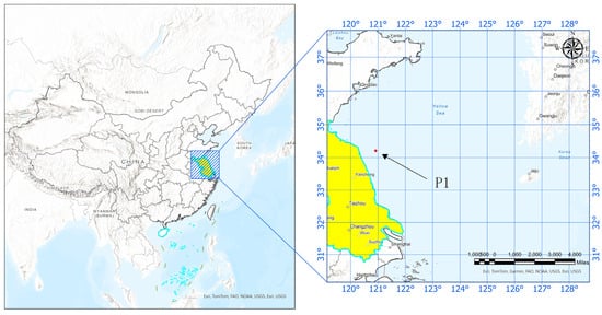
Figure 1.
Map of measuring points in Xiangshui sea area.
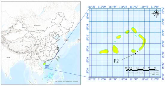
Figure 2.
Map of measuring points in Xisha sea area.

Table 1.
Summary of wave data.
2.2. Data Pre-Processing and Classification
First, according to the screening criteria in Section 2.1, the fast Fourier Transform (FFT) is applied to the 9853 eligible original bimodal wave data to obtain the original wave spectra. The duration of the record segment used for the Fourier transform is 1024 s. Subsequently, the obtained original wave spectra are smoothed using the rectangular window formula with a width of 0.2931 Hz.
Secondly, the wave observation data indicate that most waves appear in the form of mixed waves (both wind waves and swell waves coexist on the sea surface). The spectral structure of mixed waves is complex and diverse. In most cases, the wave spectra exhibit a bimodal shape, while in a few cases, they show a unimodal shape. In this paper, the classification method of bimodal wave spectra proposed by Liu Xiaoxia [21] is adopted to classify the smoothed bimodal wave spectra into three categories:
- The bimodal spectrum dominated by wind waves: most of the energy of the frequency spectrum is concentrated at the high-frequency peak, while the energy at the low-frequency peak is very small.
- The bimodal spectrum dominated by swell waves: the low-frequency peak of the frequency spectrum is much larger than the high-frequency peak.
- The bimodal spectrum with comparable wind and swell energy: the difference between the high-frequency and low-frequency peaks of the frequency spectrum is relatively small.
These three typical bimodal frequency spectra can be classified by the ratio of the low-frequency peak to the high-frequency peak (S1/S2). For the bimodal spectrum dominated by wind waves: 0.1 ≤ S1/S2 < 0.67; for the bimodal spectrum with comparable wind and swell energy: 0.67 ≤ S1/S2 < 1.5; for the bimodal spectrum dominated by swell waves: S1/S2 > 1.5.
According to the above classification method, after classifying the smoothed bimodal wave spectra into three categories, considering that wave spectra of the same category may have excessive scale differences (wave height, frequency range) due to different measurement points, the three types of wave spectra are successively subjected to dimensionless processing. The calculation formula is as follows:
where represents the non-dimensionalized frequency, ω represents the frequency, ωp represents the peak frequency, represents the non-dimensionalized energy density, S(ω) represents the energy density, and S(ωp) represents the spectral peak value energy density.
Finally, the three types of wave spectra after dimensionless processing are averaged (taking 10 dimensionless wave spectra in one category as a group to calculate the average value and repeating this process until a single value is obtained). Eventually, the average dimensionless wave spectrum dominated by wind waves, the average dimensionless wave spectrum dominated by swell waves, and the average dimensionless wave spectrum with comparable wind and swell energy are obtained. These are used as the sample spectra for this study. The three types of sample spectra are shown in Figure 3.
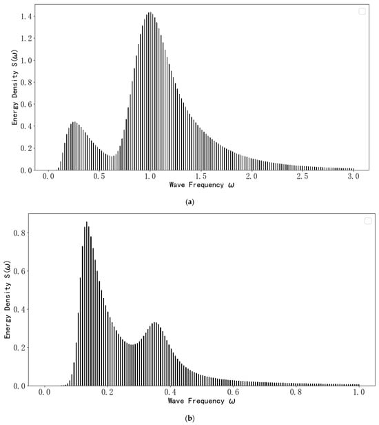
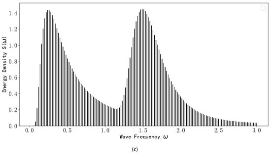
Figure 3.
Type chart of bimodal wave sample spectra. (a) The average dimensionless wave frequency spectrum dominated by wind waves. (b) The average dimensionless wave frequency spectrum dominated by swell waves. (c) The average dimensionless wave frequency spectrum with comparable energy of wind waves and swells.
3. Solving of Fitting Spectrum Parameters and Measurement of Fitting Effect
Firstly, by using the relationships between the parameters given in three types of unimodal wave spectra (the rational fraction unimodal spectrum, the Jonswap spectrum, and the Neumann spectrum) and the characteristic quantities of the sample spectrum (such as the zero-order moment m0 and the frequency corresponding to the peak value ωp, etc.), the parameters in the unimodal wave spectra are calculated, so as to obtain the specific expressions of the unimodal wave spectra.
Secondly, taking two unimodal wave spectra as the low-frequency sub-spectrum and the high-frequency sub-spectrum, respectively, a bimodal ocean wave spectrum is constructed by superimposing the low-frequency sub-spectrum and the high-frequency sub-spectrum, and the specific expression of the bimodal wave spectrum is obtained.
Finally, the bimodal wave spectrum and the sample spectrum are input into the improved particle swarm optimization (PSO) algorithm to optimize the parameters of the bimodal wave spectrum. After multiple rounds of iterative optimization, the parameter expressions of the bimodal wave spectrum with high accuracy are obtained.
3.1. Methods for Solving Parameters of Unimodal Wave Spectrum
- (1)
- Rational fractional single-peak spectrum:
- (2)
- Jonswap spectrum:
- (3)
- Neumann spectrum:
3.2. Construct Bimodal Wave Spectra
In this paper, the three wave spectra mentioned in Section 3.1 are selected as the basic components of the bimodal wave spectrum, and the bimodal wave spectrum is constructed by superimposing the low-frequency sub-spectrum and the high-frequency sub-spectrum:
where S(ω), S1(ω), S2(ω), and ω represent the bimodal wave spectrum, low-frequency sub-spectrum, high-frequency sub-spectrum, and frequency, respectively.
During the superposition process, the zero-order moments m01 and m02 of the low-frequency sub-spectrum and the high-frequency sub-spectrum are important parameters of the single-peak wave spectrum. However, the characteristic quantities of the sample spectrum cannot directly yield the values of m01 and m02; and when two single-peak wave spectra are superimposed to form a bimodal wave spectrum, there will be an issue where the energy of the high-frequency part of the bimodal wave spectrum is slightly higher than that of the sample spectrum. Therefore, the solving and iterative method proposed by [16] is employed to determine the values of m01 and m02 and to address the problem of excessive energy in the high-frequency part of the bimodal wave spectrum. The specific process is as follows:
Considering the narrow-spectrum [28,29] nature of the single-peak spectrum, some approximate assumptions can be made:
Among them, S01 and S02 represent the spectral peak energies of the low-frequency sub-spectrum and the high-frequency sub-spectrum, respectively, and m01 and m02 represent the zero-order moments of the low-frequency sub-spectrum and the high-frequency sub-spectrum, respectively. The establishment of Equation (6) needs to be based on an approximate assumption that the widths of the low-frequency sub-spectrum and the high-frequency sub-spectrum are approximately the same. The sample spectra in this study all meet this condition.
The following establishes the relationship between the characteristic quantities of the sample spectrum and the parameters of the sub-spectrum. First, Equation (7) naturally holds the following:
Among them, m01, m02, and m0 represent the zero-order moment of the low-frequency sub-spectrum, the zero-order moment of the high-frequency sub-spectrum, and the zero-order moment of the sample spectrum, respectively.
Secondly, considering the narrow-spectrum characteristics of the unimodal wave spectrum, if the two peak frequencies of the sample spectrum are far apart, then the peak frequencies of the bimodal wave spectrum have a minimal offset from the peak frequencies of the corresponding sample spectrum. Therefore, the following conclusions can be drawn:
Among them, ω01 and ω02 represent the low-frequency peak frequency and the high-frequency peak frequency of the bimodal wave spectrum, respectively, and ω1 and ω2 represent the low-frequency peak frequency and the high-frequency peak frequency of the sample spectrum, respectively.
By combining Equations (6) and (7), we can obtain
According to the fact that the low-frequency peak value of the sample spectrum is the sum of the spectral peak value of the low-frequency sub-spectrum and the spectral value of the high-frequency sub-spectrum at that position, S01 and S02 can be calculated, that is,
Similarly, for the high-frequency peak value, this should be as follows:
Since the energy of the single-peak wave spectrum is mainly concentrated around the peak frequency and S2(ω1) is close to zero, it can be assumed that S1 is contributed entirely by S01, i.e.,
However, Equation (13) should not be treated in the same way. The single-peak wave spectrum has a long tail, and when ω2 >> ω1, the contribution of S1(ω2) to S2 can be omitted, and it is sufficient to take S02 = S2; when ω2 does not differ much from ω1, S1(ω2) cannot be ignored, or else the high-frequency portion of the bimodal wave spectrum will be overestimated. Therefore, an iterative approach is used to solve this problem.
First assume that the initial iteration value is as follows:
Next, ω = ω2 is brought into S1(ω) to determine S1(ω2), which is then brought into Equation (13) to obtain the following:
According to Equation (17), this process is repeated until the desired accuracy is achieved. It is calculated that in the vast majority of cases, one iteration will satisfy the required accuracy.
Through the above method, this paper is able to accurately calculate the zero-order moments m01 and m02 of the low-frequency sub-spectrum and the high-frequency sub-spectrum based on the known characteristic quantities of the sample spectrum and properly solves the problem of the excessively high energy in the high-frequency part of the bimodal sea wave spectrum.
In addition, given that the single-peak spectrum exhibits narrow-spectrum characteristics, and according to the sample spectrum in this paper, the low-frequency peak frequency and the high-frequency peak frequency are far apart. Therefore, during the superposition process, we assume that all parameters of these two single-peak wave spectra are independent of each other. (The experimental results show that when the above two conditions are met, the fitting accuracy error of the bimodal sea wave spectrum with independent parameters is less than 5%).
3.3. Improved Particle Swarm Optimization (PSO) Algorithm
The particle swarm optimization (PSO) algorithm is an optimization algorithm based on swarm intelligence. By simulating the foraging behavior of bird flocks, it uses particles to search for optimal parameters in the solution space. Each particle represents a potential solution and has an initial position and velocity. The position and velocity of particles are updated based on individual and group experience. This paper improves the traditional PSO algorithm by adding an adaptive parameter adjustment module and a local search enhancement module to enhance the algorithm’s local search ability and the ability to explore potential optimal solutions. Moreover, in the update steps of particle positions and velocities, the overall average value is used to replace the single optimal value of each particle to prevent the particle swarm from prematurely converging around a local optimal solution. In the optimization of wave spectrum parameters, the spectrum model has multiple parameters (such as spectral peak frequency, sharpness factor, etc.). The improved PSO algorithm can iteratively adjust the parameters of the spectrum model to find a set of parameters that minimize the error between the fitted spectrum and the measured spectrum, so as to better fit the observed data.
First, initialize the PSO algorithm model. Randomly generate a set of particles (in this paper, 50 particles are generated), define the initial velocity of each particle, and set the value range of each parameter. Second, define the fitness function of the model. The fitness function measures the degree of fit between the fitted spectrum and the measured spectrum. In this paper, the mean squared error (MSE) is selected as the fitness function (the closer the MSE is to zero, the better the fitting effect):
Among them, S1(fi) represents the fitted spectrum, S2(fi) represents the sample spectrum, and fi represents the frequency. fi has the characteristic of a uniform grid distribution. That is to say, fi is uniformly distributed within a specific interval (fmin, fmax), and the frequency interval is fixed. The formula for the uniform grid distribution is as follows:
Among them, Δf represents the frequency interval and N represents the number of frequency points. In this paper, the parameters of the uniform grid distribution of fi for the three types of bimodal sample spectra are listed in Table 2.
Table 2.
Parameters of the uniform grid distribution.
Finally, update the position and velocity of the particles to obtain the final parameter values. The formulas are as follows:
where t is the number of iterations (set to 100 iterations in the text), the value of d depends on the number of parameters of the bimodal wave spectrum, and and are the velocity and position of particle i in the t-th iteration, respectively. ω is the inertia weight. (In this paper, the initial range of ω is set to be from 0.4 to 0.9. As the number of iterations increases, the value of ω will change dynamically through the adaptive parameter adjustment module during each iteration.) c1 and c2 are learning factors. (In this paper, the initial range of c1 and c2 is set to be from 0.5 to 2.5. As the number of iterations increases, the values of c1 and c2 are also dynamically adjusted through the adaptive parameter adjustment module during each iteration). γ1 and γ2 are random numbers. is the overall average value of the particle swarm, and is the historical optimal position of the swarm.
3.4. Measurement of Fitting Effect
In this study, the fitting effect of the bimodal wave spectrum is measured using three aspects, namely: the deviation index, negative correlation coefficient, and Taylor diagram.
3.4.1. Deviation Index (D.I)
The deviation index (D.I), as a measure of fitting effectiveness, is expressed as follows:
where S(ω) represents the bimodal wave spectrum, S0(ω) represents the sample spectrum, and m0 represents the zero-order moment of the sample spectrum. A D.I of 0 is a sufficient condition for the complete coincidence of the bimodal wave spectrum and the target spectrum, and the closer the D.I is to zero, the better the fitting effect.
3.4.2. Negative Correlation Coefficient R2
The negative correlation coefficient, R2, is an indicator of the degree of linear correlation between two variables, with a value between 0 and 1, expressed by the following formula:
where ŷi is the predicted value, yi is the measured value, and is the mean of the measured values.
In practical applications, the value of R2 can be used to evaluate the fitting degree of the wave model. The closer R2 is to 1, the better the wave model fits the sample data. On the contrary, the closer it is to 0, the poorer the wave model’s ability to explain the sample data.
3.4.3. Taylor Diagram
A Taylor diagram is a tool for evaluating the accuracy of a model by graphically displaying three important accuracy metrics: the correlation coefficient, the standard deviation, and the root mean square error. In a Taylor diagram, the horizontal and vertical axes indicate the standard deviation of the fitted and sample values, respectively. The radial line indicates the correlation coefficient. The dashed lines indicate the root mean square error. Taylor diagrams serve as an intuitive visualization tool to visualize the accuracy, bias, and uncertainty of model predictions. By comparing the positions of different models on the Taylor diagram, one can quickly identify which models perform better in the three areas mentioned above.
4. Comparison Results of the Fitted Spectra
In this paper, three types of bimodal wave spectra are constructed in the manner described in Section 3.2, which are the following, respectively:
Fitted Spectrum 1: Rational fractional single-peak spectrum + rational fractional single-peak spectrum:
Fitted Spectrum 2: Rational fractional single-peak spectrum + Jonswap spectrum:
Fitted Spectrum 3: Rational fractional single-peak spectrum + Neumann spectrum:
Fit the three types of sample spectra obtained in Section 2.2 with the above three fitting spectra, respectively. At the same time, use the Huang Peiji six-parameter spectrum, Shen Zhichun spectrum, and Ochi-Hubble spectrum, which have relatively good fitting effects in the South China Sea, as the comparative wave spectra, so as to observe the fitting effects and find the fitting spectrum with the best performance.
4.1. Fit the Bimodal Spectrum Dominated by Wind Waves
According to the parameter-solving methods proposed in Section 3.1, Section 3.2 and Section 3.3, the precise parameters of Fitted Spectrum 1, Fitted Spectrum 2, and Fitted Spectrum 3 are obtained. The parameter table is presented in Table 3.
Table 3.
Fitted spectrum parameters (bimodal spectrum dominated by wind waves).
The Fitted Spectra 1–3, Huang Peiji six-parameter spectrum, Shen Zhichun spectrum, and Ochi-Hubble spectrum are fitted with the bimodal sample spectrum dominated by wind waves. The observed effects are shown in Figure 4, and the fitting effects are presented in Table 4.
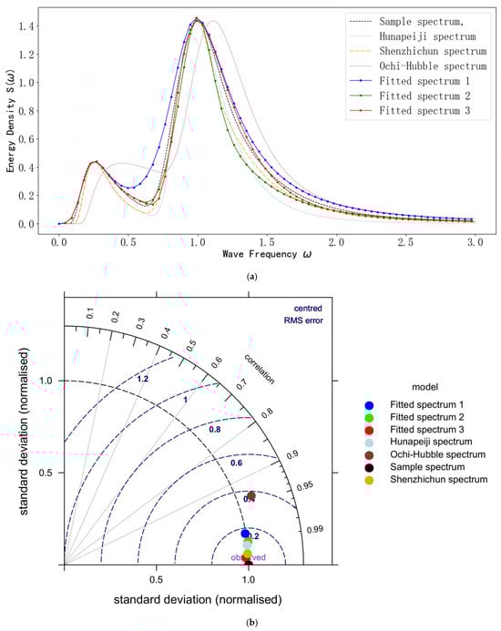
Figure 4.
Fitting effect diagram (dominated by wind waves). (a) Fitting diagram of the wind-wave-dominated bimodal spectrum. (b) Taylor chart for observing the fitting effect.
Table 4.
Comparison of fitting effects (bimodal spectrum dominated by wind waves).
As can be seen from Figure 4a, the energy in the low-frequency part, high-frequency part, and trough of the spectrum fitted by the Huang Peiji spectrum and the Shen Zhichun spectrum is less than that of the sample spectrum. The energy of the Ochi-Hubble spectrum is shifted to the right as a whole compared with the sample spectrum, and the energy of the trough is too large. Therefore, it is only used as a reference. When comparing Fitted Spectrum 1 with the sample spectrum, its fitting effect is good in the frequency range of 0–0.4, and the energy shape is close to that of the sample spectrum. However, when fitting the energy of the high-frequency part and the trough, the energy of Fitted Spectrum 1 is significantly greater than that of the sample spectrum. Therefore, Fitted Spectrum 1 is not applicable. When comparing Fitted Spectrum 2 with the sample spectrum, its fitting effect is good when fitting the energy of the low-frequency part, the trough, and the first half of the high-frequency part, and the energy shape is close to that of the sample spectrum. However, when fitting the energy of the second half of the high-frequency part, the energy of Fitted Spectrum 2 is too small compared with the sample spectrum. Therefore, it is not applicable. When comparing Fitted Spectrum 3 with the sample spectrum, the energies of its fitted low-frequency part, high-frequency part, and trough all show good results compared with the sample spectrum, and its energy shape basically coincides with that of the sample spectrum.
In the Taylor diagram, the closer the distance between the model point and the observation point (in the Taylor diagram of this paper, the black dot (sample spectrum) represents the observation point), the closer the standard deviation and root mean square error of the model are to the observed data and the lower the model error is, indicating a better fitting effect. The larger the angle between the model point and the polar axis (in the Taylor diagram of this paper, the polar axis is the positive direction of the y-axis), the higher the model correlation is. We will not elaborate on this property here.
As can be seen from Figure 4b, the distance between Fitted Spectrum 1 and the observation point (sample spectrum) is 0.17, and the angle with the polar axis is 0.98. The distance between Fitted Spectrum 2 and the observation point is 0.15, and the angle with the polar axis is 0.99. The distance between Fitted Spectrum 3 and the observation point is 0.025, and the angle with the polar axis is 0.998. The distance between the Huang Peiji spectrum and the observation point is 0.1, and the angle with the polar axis is 0.996. The distance between the Ochi-Hubble spectrum and the observation point is 0.38, and the angle with the polar axis is 0.94. The distance between the Shen Zhichun spectrum and the observation point is 0.05, and the angle with the polar axis is 0.996. Therefore, it can be concluded that the red dot representing Fitted Spectrum 3 is the closest to the observation point and has the largest angle with the polar axis, indicating that Fitted Spectrum 3 has the lowest model error, the highest correlation with the sample spectrum, and the best fitting effect.
As can be seen from Table 4, the D.I value of Fitted Spectrum 3 (the closer it is to 0, the better the fitting effect) is the smallest, with a value of 0.07, and the R2 value (the closer it is to 1, the better the fitting effect) is the largest, with a value of 0.99. Combining the D.I value and the R2 value, it can be concluded that Fitted Spectrum 3 has the best fitting effect.
In conclusion, based on the conclusions of Figure 4a,b and Table 4, when fitting the bimodal sample spectrum dominated by wind waves, the energy shape of Fitted Spectrum 3 is the closest to that of the sample spectrum, and in terms of standard deviation, D.I value, R2 value, etc., it is superior to Fitted Spectrum 1, Fitted Spectrum 2, the Huang Peiji spectrum, the Shen Zhichun spectrum, and the Ochi-Hubble spectrum. Therefore, Fitted Spectrum 3 has the best fitting effect.
4.2. Fit the Bimodal Spectrum Dominated by Swell Waves
Fit Fitted Spectra 1–3, the Huang Peiji six-parameter spectrum, the Shen Zhichun spectrum, and the Ochi-Hubble spectrum with the bimodal sample spectrum dominated by swell waves. The precise parameters of the Fitted Spectra 1–3 are shown in Table 5. The observation results are shown in Figure 5, and the fitting effects are shown in Table 6.
Table 5.
Fitted spectrum parameters (bimodal spectrum dominated by swell waves).
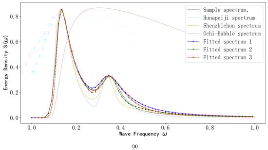
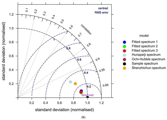
Figure 5.
Fitting effect diagram (dominated by swell waves). (a) Fitting diagram of the swell-wave-dominated bimodal spectrum. (b) Taylor chart for observing the fitting effect.
Table 6.
Comparison of fitting effects (bimodal spectrum dominated by swell waves).
As can be seen from Figure 5a, when the Huang Peiji spectrum and the Shen Zhichun spectrum are used to fit the bimodal sample spectrum dominated by swell waves, the energy fitting effect of the low-frequency part is good. However, the Huang Peiji spectrum again has the problem that the energy of the trough is much smaller than that of the sample spectrum, and the Shen Zhichun spectrum again has the problem that both the energy of the trough and the energy of the high-frequency part are smaller than those of the sample spectrum. When the Ochi-Hubble spectrum is used to fit the sample spectrum, its energy is completely out of control, so it is not taken into consideration. When comparing Fitted Spectrum 2 with the sample spectrum, the energies of its fitted low-frequency part, high-frequency part, and trough all show good results compared with the sample spectrum, and the energy shapes are basically consistent with that of the sample spectrum. The energy shapes of Fitted Spectrum 1 and Fitted Spectrum 3 are relatively close to that of the sample spectrum. However, the energy of the trough and the energy of the high-frequency part of Fitted Spectrum 1 are slightly greater than those of the sample spectrum. The energy of the trough of Fitted Spectrum 3 is slightly smaller than that of the sample spectrum, and the energy of the high-frequency part is slightly greater than that of the sample spectrum. Although the fitting effects of the two are relatively good, they are slightly inferior compared to Fitted Spectrum 2.
As can be seen from Figure 5b, the distance between Fitted Spectrum 1 and the observation point is 0.13, and the angle with the polar axis is 0.992. The distance between Fitted Spectrum 2 and the observation point is 0.08, and the angle with the polar axis is 0.996. The distance between Fitted Spectrum 3 and the observation point is 0.11, and the angle with the polar axis is 0.994. The distance between the Huang Peiji spectrum and the observation point is 0.33, and the angle with the polar axis is 0.96. The distance between the Shen Zhichun spectrum and the observation point is 0.26, and the angle with the polar axis is 0.97. Therefore, it can be concluded that the green dot representing Fitted Spectrum 2 is the closest to the observation point and has the largest angle with the polar axis, indicating that the Fitting Spectrum 2 has the lowest model error, the highest correlation with the sample spectrum, and the best fitting effect.
As can be seen from Table 6, the D.I value of Fitted Spectrum 2 is the smallest, with a value of 0.10, and the R2 value is the largest, with a value of 0.99. Combining the D.I value and the R2 value, it can be concluded that the fitting effect of Fitted Spectrum 2 is the best.
In summary, according to the conclusions of Figure 5a,b and Table 6, when Fitted Spectrum 2 is used to fit the bimodal sample spectrum dominated by swell waves, its energy shape is the closest to that of the sample spectrum, and in terms of the standard deviation, D.I value, R2 value, etc., it is superior to Fitted Spectrum 1, Fitted Spectrum 3, the Huang Peiji spectrum, the Shen Zhichun spectrum, and the Ochi-Hubble spectrum. Therefore, the fitting effect of Fitted Spectrum 2 is the best.
4.3. Fit the Bimodal Spectrum with Comparable Wind and Swell Energy
Fit Fitted Spectra 1–3, the Huang Peiji six-parameter spectrum, the Shen Zhichun spectrum, and the Ochi-Hubble spectrum with the bimodal sample spectrum with comparable wind and swell energy. The precise parameters of Fitted Spectra 1–3 are shown in Table 7. The observation results are shown in Figure 6, and the fitting effects are shown in Table 8.
Table 7.
Fitted spectrum parameters (the bimodal spectrum with comparable wind and swell energy).
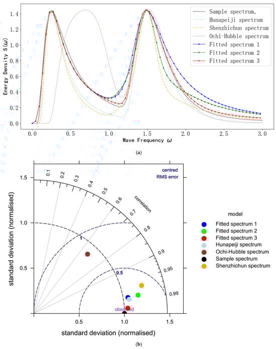
Figure 6.
Fitting effect diagram (with comparable wind and swell energy). (a) The fitting diagram of the bimodal spectrum with comparable wind and swell energy. (b) Taylor chart for observing the fitting effect.
Table 8.
Comparison of fitting effects (the bimodal spectrum with comparable wind and swell energy).
As can be seen from Figure 6a, when the Huang Peiji spectrum is used to fit the bimodal sample spectrum with comparable wind and swell energy, the energy in the second half of the low-frequency part, the energy of the trough, and the energy of the high-frequency part are all smaller than those of the sample spectrum. When comparing the Shen Zhichun spectrum with the sample spectrum, the energy in the second half of the low-frequency part and the high-frequency energy are much smaller than those of the sample spectrum, resulting in a poor fitting effect. When the Ochi-Hubble spectrum is used to fit the sample spectrum, the fitting effect of the high-frequency part is good, but the energy in the low-frequency part is out of control, so it is not taken into consideration. The energy shapes of the low-frequency parts of Fitted Spectrum 1 and Fitted Spectrum 2 are relatively close to that of the sample spectrum, but the energy of the trough and the energy of the high-frequency part of Fitted Spectrum 1 are both greater than those of the sample spectrum; the energy of the trough of Fitted Spectrum 2 is greater than that of the sample spectrum, and there is a large deviation in the energy of the second half of the high-frequency part compared with the sample spectrum. Therefore, Fitted Spectrum 1 and Fitted Spectrum 2 are not applicable. When comparing Fitted Spectrum 3 with the sample spectrum, the fitted energy of the low-frequency part, the energy of the high-frequency part, and the energy of the trough all show good results compared with the sample spectrum, and the energy shape is very close to that of the sample spectrum.
As can be seen from Figure 6b, the distance between Fitted Spectrum 1 and the observation point is 0.22, and the polar axis angle is 0.985. The distance between Fitted Spectrum 2 and the observation point is 0.27, and the polar axis angle is 0.987. The distance between Fitted Spectrum 3 and the observation point is 0.08, and the polar axis angle is 0.998. The distance between the Huang Peiji spectrum and the observation point is 0.21, and the polar axis angle is 0.99. The distance between the Ochi-Hubble spectrum and the observation point is 0.59, and the polar axis angle is 0.67. The distance between the Shen Zhichun spectrum and the observation point is 0.38, and the polar axis angle is 0.97. Therefore, it can be concluded that the red point representing Fitted Spectrum 3 is the closest to the observation point and has the largest polar axis angle, indicating that the model error of Fitted Spectrum 3 is the lowest, and it has the highest correlation with the sample spectrum and the best fitting effect.
As can be seen from Table 8, the D.I value of Fitted Spectrum 3 is the smallest, with a value of 0.09, and the R2 value is the largest, with a value of 0.99. Combining the D.I value and the R2 value, it can be concluded that Fitted Spectrum 3 has the best fitting effect.
In summary, according to the conclusions of Figure 6a,b and Table 8: When Fitted Spectrum 3 is used to fit the bimodal sample spectrum with comparable wind and swell energy, its energy shape is the closest to that of the sample spectrum, and in terms of standard deviation, D.I value, R2 value, etc., it is superior to Fitted Spectrum 1, Fitted Spectrum 2, the Huang Peiji spectrum, the Shen Zhichun spectrum and the Ochi-Hubble spectrum. Therefore, Fitted Spectrum 3 has the best fitting effect.
According to the research of this paper and combined with the above experimental results, it shows that when the Huang Peiji spectrum and the Shen Zhichun spectrum are used to fit the three types of sample spectra, their D.I values and R2 values are relatively good, but there is still a large gap between their energy shapes and those of the sample spectra. When fitting the bimodal spectrum dominated by wind waves and the bimodal spectrum with comparable wind and swell energy, Fitted Spectrum 3 proposed in this paper (that is, the rational fractional unimodal spectrum + Neumann spectrum) has achieved satisfactory fitting effects both in terms of the energy shape and numerical values such as the D.I value. When fitting the bimodal spectrum dominated by swell waves, Fitted Spectrum 2 proposed in this paper (that is, the rational fractional unimodal spectrum + Jonswap spectrum) has also achieved very satisfactory fitting effects in terms of the energy shape and numerical values such as the D.I value. After multiple calculations, it is found that in this study, when the Ochi-Hubble spectrum is used to fit the bimodal spectrum dominated by swell waves, a unimodal result is obtained. When fitting the other two types of bimodal spectra, there is a large difference between the energy shape of the Ochi-Hubble spectrum and that of the sample spectrum. This difference may be caused by the small value of the peak frequency of the low-frequency spectrum of the target spectrum. Therefore, the values of the Ochi-Hubble spectrum are for reference only.
5. Discussion
In this paper, the fitting method for double-peaked wave spectra is successfully constructed and validated based on the measured wave data from Jiangsu Ringshui station and Xisha sea area. The results show that the fitting spectrum model with rational fractional single-peak spectra, Neumann spectra, and Jonswap spectra superimposed performs well in fitting the double-peak wave spectra, and the fitting efficiency reaches up to 99%. This finding not only verifies the effectiveness of the proposed method but also provides important theoretical support for the reconstruction of bimodal wave spectra in domestic island regions.
5.1. Comments on Ochi-Hubble Spectrum
In comparison with other high-precision bimodal fitting spectra (Huang Peiji six-parameter spectra, Ochi-Hubble spectra, and Shen Zhichun fitting spectra), there are some limitations in the performance of Ochi-Hubble spectra. In this paper, it is found that the Ochi-Hubble spectrum tends to generate only single-peak spectra when fitting swell-dominated bimodal spectra and is unable to accurately capture the bimodal features. In addition, when fitting the other two types of bimodal spectra, the peak frequency of the low-frequency part has a large deviation from the theoretical value, especially when the low-frequency peak frequency is small. This deviation may be related to the parameterization method of the Ochi-Hubble spectrum and its sensitivity to the low-frequency energy distribution. Therefore, although the Ochi-Hubble spectrum has some reference value in some cases, its applicability in the complex sea state of the South China Sea islands and reefs is limited.
5.2. Combination of Rational Fraction Single-Peak Spectra and Neumann Spectra
The results show that when the rational fractional unimodal spectrum is used as the low-frequency component and combined with the Neumann spectrum as the high-frequency component, the fitting accuracy of the bimodal spectrum can be significantly improved. This combination can not only accurately capture the energy distribution of wind waves and swell waves, but also effectively fit the peak frequency and energy concentration region of the bimodal spectrum. Especially when fitting the bimodal spectrum dominated by wind waves and the bimodal spectrum with comparable wind and swell energy, this combination outperforms other models, with a fitting efficiency of up to 99%. However, in the bimodal spectrum dominated by swell waves, although the Neumann spectrum performs well, there is still a certain deviation in the fitting results, and its fitting ability in the high-frequency part still needs to be further optimized.
5.3. Applicability Analysis of the Jonswap Spectrum
When fitting the bimodal spectrum dominated by swell waves, the fitting effect of the Jonswap spectrum as a high-frequency component is better than that of the Neumann spectrum, and the fitting accuracy can reach 99%. However, when fitting the bimodal spectrum dominated by wind waves and the bimodal spectrum with comparable wind and swell energy, the fitting error of the Jonswap spectrum is relatively large, indicating its limited applicability. This limitation may be related to the spectral peak enhancement factor γ in the Jonswap spectrum. Therefore, when applying the Jonswap spectrum to the complex sea conditions of the islands and reefs in the South China Sea of China, further optimization is still needed.
5.4. Extension to Areas Beyond the Data Collection Point
The results of this study are applicable not only to the measured data in the offshore area of Rudong, Jiangsu Province, and the waters near the Xisha Islands, but also can serve as a reference for the research on bimodal wave spectra in other island–reef waters of the South China Sea. The South China Sea islands and reefs have complex terrains and diverse wave types. The fitting accuracy of bimodal wave spectra directly impacts the data support for aspects such as ocean engineering, weather forecasting, and navigation safety. August is a peak season for typhoon weather in the South China Sea. Due to practical constraints, this paper can only obtain the wave data of the South China Sea in August. The waters of Xiangshui, Jiangsu Province enjoy a relatively mild climate throughout the year, and their wave patterns are quite similar to those of the South China Sea during the non-typhoon period. Therefore, the sea conditions in the Xiangshui waters are regarded as typical sea conditions of the South China Sea during the non-typhoon period. There are numerous islands and reefs in the South China Sea region. Through analysis, it has been found that the characteristics of bimodal waves near these islands and reefs are highly similar to the wave data of the selected measurement points in the South China Sea. This discovery further validates the universality of the research results. By extending the combination method of the rational-fraction single-peak spectrum and the Neumann spectrum to other regions, the fitting accuracy of the bimodal wave spectrum can be further improved, providing a more reliable theoretical basis for marine scientific research in the South China Sea island and reef region.
5.5. Research Limitations and Future Perspectives
Although this study achieved good results in the fitting of bimodal wave spectra, there are still some limitations. For example, although Fitted Spectrum 2 performs well when fitting the bimodal spectrum dominated by swell waves, it is inferior to Fitted Spectrum 3 when fitting the bimodal spectrum dominated by wind waves and the bimodal spectrum with similar wind and swell energy. This indicates that the universality of Fitted Spectrum 2 still needs to be improved. In addition, the Ochi-Hubble and Jonswap spectra have limited applicability under specific conditions, and future studies can explore more flexible parameterization methods or introduce new machine learning algorithms to optimize the model performance. Meanwhile, further expanding the data collection scope to cover more measured data in the South China Sea islands and reefs will help to verify the generalizability of the model and improve its prediction accuracy.
6. Conclusions
Considering the complexity of the sea state in the island–reef region of the South China Sea, the island–reef waves are influenced by the topography, which imparts strong nonlinearity and weak dispersion. When wind waves and swells occur simultaneously, the waves often exhibit double-peak or even multi-peak characteristics. Currently, wave spectrum studies mainly focus on single-peak waves, while studies on double-peak wave spectrum are less researched. Therefore, researching double-peak wave spectrum is benefice for more accurately describing the complex sea state. This research provides new ideas and references for research and practice in the fields of wave theory and nearshore engineering.
In this paper, actual wave data collected near the Xisha Islands in August 2014 and at the Jiangsu Xiangshui station in 2017 are used. The waves are categorized into three spectral types based on their characteristics: the double-peak spectrum with the wind wave dominating, the double-peak spectrum with the swell wave dominating, and the double-peak spectrum with the strength of wind wave is close to that of the swell. According to the wave characteristics of the island–reef area, the rational fractional single-peak spectrum, Neumann spectrum, and Jonswap spectrum are used to fit the above three spectral types. These fits are then compared with the Huang Peiji six-parameter spectrum, Ochi-Hubble spectrum, and Shen Zhichun fitting spectrum. The fitting effects are observed through three aspects. The results show that when fitting the bimodal spectrum dominated by wind waves and the bimodal spectrum with comparable wind and swell energy, using the rational fractional single-peak spectrum as the low-frequency component and Neumann spectrum as the high-frequency component can achieve a more satisfactory fitting effect, with the fitting accuracy reaching 99%. Although the Jonswap spectrum, as a high-frequency component, performs well when fitting the bimodal spectrum dominated by swell waves, there is still a large error when fitting the bimodal spectrum dominated by wind waves and the bimodal spectrum where the strength of the wind wave is close to that of the swell. Therefore, it is not applicable to all spectral types. The research results of this paper lay the foundation for the accurate characterization of wave spectra in the island–reef waters of the South China Sea and provide valuable references for subsequent studies.
However, the interactions between the parameters of the wave spectrum lead to errors in the fitting of the two single-peak spectra in the overlapping region. Further research and improvements are needed to improve the accuracy of the model.
Author Contributions
Methodology, L.Q.; Software, W.S.; Formal analysis, W.S.; Investigation, X.W.; Resources, Y.P.; Data curation, X.W.; Writing—original draft, W.S.; Visualization, W.S.; Supervision, Y.P. and L.Q.; Funding acquisition, Y.P. and L.Q. All authors have read and agreed to the published version of the manuscript.
Funding
This research is supported by the Liaoning Provincial Education Department Basic Research Project (Project No. LJKMZ20221115), National Natural Science Foundation of China (Project No. 51975032), and National Natural Science Foundation of China Major Project (Project No. 51939003). The authors also express their deep gratitude to the editors and reviewers for their careful reading, suggestions, and comments on the manuscript.
Institutional Review Board Statement
Not applicable.
Informed Consent Statement
Not applicable.
Data Availability Statement
The data supporting the findings of this study are of a semi-confidential nature and cannot be made publicly available due to privacy and security concerns. Access to the data is restricted, and any requests for data sharing will be considered on a case-by-case basis, subject to approval by the relevant institutional review boards and data protection authorities.
Conflicts of Interest
The authors declare no conflicts of interest.
References
- Moskowitz, L. Estimates of the power spectrums for fully developed seas for wind speeds of 20 to 40 knots. J. Geophys. Res. Atmos. 1964, 69, 5161–5179. [Google Scholar] [CrossRef]
- Goda, Y. A comparative review on the functional forms of directional wave spectrum. Coast. Eng. J. 1999, 41, 9900002. [Google Scholar] [CrossRef]
- Tanaka, M. Report of Seakeeping Committee. In Proceedings of the 15th International Towing Tank Conference, The Hague, The Netherlands, 3–10 September 1978. [Google Scholar]
- Ochi, M.K.; Hubble, E.N. Six-parameter wave spectra. Coast. Eng. Proc. 1976, 1, 17. [Google Scholar] [CrossRef]
- Torsethaugen, K. Two-peak wave spectrum model. In Proceedings of the 12th OMAE Conference, Glasgow, UK, 20–24 June 1993. [Google Scholar]
- Torsethaugen, K.; Haver, S.; Norway, S. Simplified double peak spectral model for ocean waves. In Proceedings of the Fourteenth International Offshore and Polar Engineering Conference, Toulon, France, 23–28 May 2004; International Society of Offshore and Polar Engineers: Mountain View, CA, USA, 2004. [Google Scholar]
- Akbari, H.; Panahi, R.; Amani, L. A double-peaked spectrum for the northern parts of the gulf of oman: Revisiting extensive field measurement data by new calibration methods. Ocean Eng. 2019, 180, 187–198. [Google Scholar] [CrossRef]
- Garcia-Gabin, W. Wave bimodal spectrum based on swell and wind-sea components. Ifac Pap. 2015, 48, 223–228. [Google Scholar] [CrossRef]
- Rossi, G.B.; Crenna, F.; Berardengo, M.; Piscopo, V.; Scamardella, A. Investigation on Spectrum Estimation Methods for Bimodal Sea State Conditions. Sensors 2021, 21, 2995. [Google Scholar] [CrossRef]
- Welch, P.D. The Use of Fast Fourier Transform for the Estimation of Power Spectra: A Method Based on Time Averaging over Short Modified Periodograms. IEEE Trans. Audio Electroacoust. 1967, 15, 70–73. [Google Scholar] [CrossRef]
- Thomson, D.J. Spectrum Estimation and Harmonic Analysis. Proc. IEEE 1982, 70, 1055–1096. [Google Scholar] [CrossRef]
- Deng, F.; Wang, J.; Wang, J. Estimation of a five-parameter JONSWAP spectra with an improved particle swarm optimization. Appl. Ocean. Res. 2023, 136, 103580. [Google Scholar] [CrossRef]
- Kennedy, J.; Eberhart, R. Particle Swarm Optimization. In Proceedings of the IEEE International Conference on Neural Networks (ICNN), Perth, WA, Australia, 27 November–1 December 1995; pp. 1942–1948. [Google Scholar]
- Rueda-Bayona, J.G.; Guzmán, A.; Silva, R. Genetic algorithms to determine jonswap spectra parameters. Ocean Dyn. 2020, 70, 561–571. [Google Scholar] [CrossRef]
- Rueda-Bayona, J.G.; Guzmán, A.F.; Eras, J.J.C. Selection of jonswap spectra parameters during water-depth and sea-state transitions. J. Waterw. Port Coast. Ocean Eng. 2020, 146, 04020038. [Google Scholar] [CrossRef]
- Guan, C.; Zhang, D.; Guan, S. Repersentation of bimodal frequency spectra of sea waves. Ocean Lakes 1996, 27, 151–156. [Google Scholar]
- Liu, X. Numerical Simulation of Freak Waves in Three-Dimensional Waves Field. Master’s Thesis, Dalian University of Technology, Dalian, China, 2008. [Google Scholar]
- Huang, P.; Hu, J. A fitting model of frequency spectrum for wind-genera the waves in Jiaozhou Bar. Yellow Sea Bohai Sea 1987, 5, 1–7. [Google Scholar]
- Huang, P.; Hu, J. Representation of the bimodal wave spectrum in Jiaozhou Bay. J. Oceanol. 1988, 10, 531–537. [Google Scholar]
- Shen, Z.; Tao, A.; Li, X. Study on standard double-peak spectrum based on observed data. Mar. Lakes Bull. 2020, 1, 9–17. [Google Scholar] [CrossRef]
- Zong, Z.; Wang, Y.; Gu, X. Study on the rational form of wave spectrum near islands and reefs. J. Hydrodyn. A 2018, 33, 570–575. [Google Scholar] [CrossRef]
- Wang, Y.; Zong, Z. Study on rational fraction spectrum of random waves in waters near islands and reefs. Dalian Univ. Technol. 2022, 61, 89–102. [Google Scholar]
- Liu, X.; Chen, W.; Sun, Z.; Cai, Z.; Hou, Y. Investigation on the reconstruction of wave bimodal spectrum in the lagoon near islands and reefs. Ocean Eng. 2022, 45, 123–135. [Google Scholar] [CrossRef]
- Chen, J.; Liu, L.; Wang, X.; Li, J.; Yao, X. Numerical simulation of bimodal wave spectrum based on viscous cfd method. In Proceedings of the International Conference on Offshore Mechanics and Arctic Engineering-OMAE, Hamburg, Germany, 5–10 June 2022; Volume 7. [Google Scholar] [CrossRef]
- Ren, X.; Xie, B.; Song, Z. Statistical characteristics of the double-peakeed wave spectra in the deep area of the South China Sea. Adv. Ocean Sci. 2014, 32, 148–154. [Google Scholar]
- Hou, Y.; Wen, S. Wind wave spectra with three parameters. Ocean Lakes 1990, 21, 495–505. [Google Scholar]
- Hong, G.; Xia, Q. About the Jonswap spectrum of wind and wave. In Proceedings of the 7th National Symposium on Coastal Engineering, Zhuhai, China, 13 November 1993; Volume 2, pp. 979–989. [Google Scholar]
- Hong, G. Exploration of some issues on the statistical nature and statistical methods of shallow water wind and waves. J. East China Inst. Water Resour. 1978, 1, 15–45. [Google Scholar]
- Hong, G. Exploration of some issues on the statistical nature and statistical methods of shallow water wind and waves (continued). J. East China Inst. Water Resour. 1978, 2, 50–71. [Google Scholar]
Disclaimer/Publisher’s Note: The statements, opinions and data contained in all publications are solely those of the individual author(s) and contributor(s) and not of MDPI and/or the editor(s). MDPI and/or the editor(s) disclaim responsibility for any injury to people or property resulting from any ideas, methods, instructions or products referred to in the content. |
© 2025 by the authors. Licensee MDPI, Basel, Switzerland. This article is an open access article distributed under the terms and conditions of the Creative Commons Attribution (CC BY) license (https://creativecommons.org/licenses/by/4.0/).