Article

Prescribed-Time Formation Tracking Control for Underactuated USVs with Prescribed Performance

College of Weaponry Engineering, Naval University of Engineering, Wuhan 430033, China
*
Author to whom correspondence should be addressed.
J. Mar. Sci. Eng. 2025, 13(3), 480; https://doi.org/10.3390/jmse13030480
Submission received: 8 February 2025 / Revised: 20 February 2025 / Accepted: 27 February 2025 / Published: 28 February 2025

Abstract

:
This article proposes a prescribed-time formation tracking control scheme for USVs with prescribed performance constraints to address the issue of multiple underactuated USV formation tracking control with external environmental disturbances and input saturation. Initially, a prescribed-time extended state observer was constructed, capable of promptly estimating and compensating for speed and external disturbances within a certain timeframe. Additionally, a unique performance function was developed, enabling the performance function to converge to a predetermined accuracy within a specified time, while allowing for flexible adjustment of the performance constraint shape by parameter modification. Furthermore, a prescribed-time formation control algorithm was developed by combining graph theory and dynamic surface control, enabling the formation error to converge within preset performance constraints at a specified period of T = 10   s . It was proved that all signals in the closed-loop system are uniform, ultimately bounded by Lyapunov stability theory and the formation tracking errors display prescribed-time stability. Finally, the efficacy and superiority of the designed control scheme were evaluated by constructing numerical simulations.

1. Introduction

With the rapid advancement of technology, unmanned surface vessels (USVs), as a novel category of water platform, are assuming an increasingly significant role in ocean exploration, surveillance, rescue, and other fields [1,2,3]. However, when facing complex environments and diverse operational tasks, the operational capability of a single USV is extremely limited, and multiple USV collaborative control has gradually become a research hotspot owing to its significant efficiency, high adaptability, and excellent resilience [4]. In the field of multiple USV collaborative control, formation tracking control is one of the significant research hotspots, and its main strategies include consistency-based strategy [5,6], behavior-based strategy [7,8], leader–follower strategy [9,10], virtual structure strategy [11,12], etc. The leader–follower control technique is defined by a straightforward control structure and excellent scalability, which has led to its widespread use. In this strategy, the following USVs only require receiving dynamic information from the leading USV to achieve a stable formation.
The trajectory tracking control of USV formation is one of the key issues in multi-USV collaborative control. By controlling the preset formation layout or changing the expected formation maneuvering trajectory, individual movements in the USV cluster can be coordinated to adapt to different mission requirements [13]. However, in actual navigation, there are often disturbances from time-varying unknown factors, which will seriously affect the control accuracy and stability of USVs. Ref. [14] propose a nonlinear extended state observer that effectively mitigates the impact of model uncertainty and external disturbances on the control system. Ref. [15] designed a formation controller based on virtual structure strategy, which transforms the formation control problem into a problem of tracking the position of virtual structure points, reducing the complexity of the control algorithm. Ref. [16] examined the distributed formation control of USVs using input and state quantization, formulating a control rule within the quantized environment to facilitate the tracking of the specified kinematic guidance signal. To achieve autonomous collaborative formation control of underactuated USVs in complex marine environments, ref. [17] proposes a dual model predictive control (DMPC) method based on virtual trajectories, in which the stability of the proposed model predictive control method in finite time domain was demonstrated by constructing a Lyapunov function. A tracking controller for decentralized output-feedback formation was suggested by combining dynamic surface control technology, backstepping program, neural network-based observer, tan-type barrier Lyapunov function, and control Lyapunov function, achieving boundedness of closed-loop signals [18]. The previously mentioned control techniques may alone attain asymptotic stability of the controller, meaning the controller converges to zero exclusively as time approaches infinity. Consequently, ref. [19] presents a distributed bearing-based formation control strategy that ensures finite-time convergence, allowing formation tracking errors to diminish within a specified timeframe. For the multi-USV formation control task under directed communication, ref. [20] proposes an adaptive nonsingular finite-time formation controller to achieve formation tracking control in finite time. However, a significant drawback of finite-time control theory is that the convergence time of the system usually depends on the initial state of the system. This means that for different initial conditions, the system may need a different time to reach a stable state, which may lead to the uncertainty of the control effect in practical applications, especially when the initial state changes greatly. To solve the above issue, ref. [21] constructs a fixed-time adaptive output feedback fault-tolerant controller. The proposed formation control algorithm can guarantee that all signals in multiple USVs systems are bounded in a fixed time. Ref. [22] studied the fixed-time USV formation control algorithm with external disturbances, and integrated an event-triggered strategy into a controller to reduce the communication burden. The convergence time of the fixed-time algorithm still relies on control parameters even if it is independent of the system’s initial state. In addition, the convergence time of fixed time control algorithms cannot be predefined, which is not conducive to practical applications. Ref. [23] propose a prescribed-time control algorithm, the key of which is that it can make the system output converge to the desired trajectory within the prescribed time without relying on the initial state and design parameter parameters of the system.
Based on the above discussion, this paper proposes a distributed USV formation control scheme by integrating graph theory, dynamic surface control algorithm, a prescribed-time approach, and prescribed-performance technique. The main advantages lie in the following aspects: graph theory can accurately describe the communication topology and information transmission, thereby enhancing communication connectivity and coordination. The dynamic surface control algorithm can improve system stability and response capability. The combination of these two enables distributed control, thereby enhancing the adaptability of the mission and the reliability of the system. This article delineates its main contributions as follows:
(1)
A distributed prescribed-time control strategy is introduced for achieving formation among underactuated USVs. This scheme guarantees that, despite the presence of unknown USV velocities, the tracking errors converge to a preset range within a certain timeframe.
(2)
A unique performance function is intended to ensure guaranteed transient and steady-state performance within a certain timeframe.
(3)
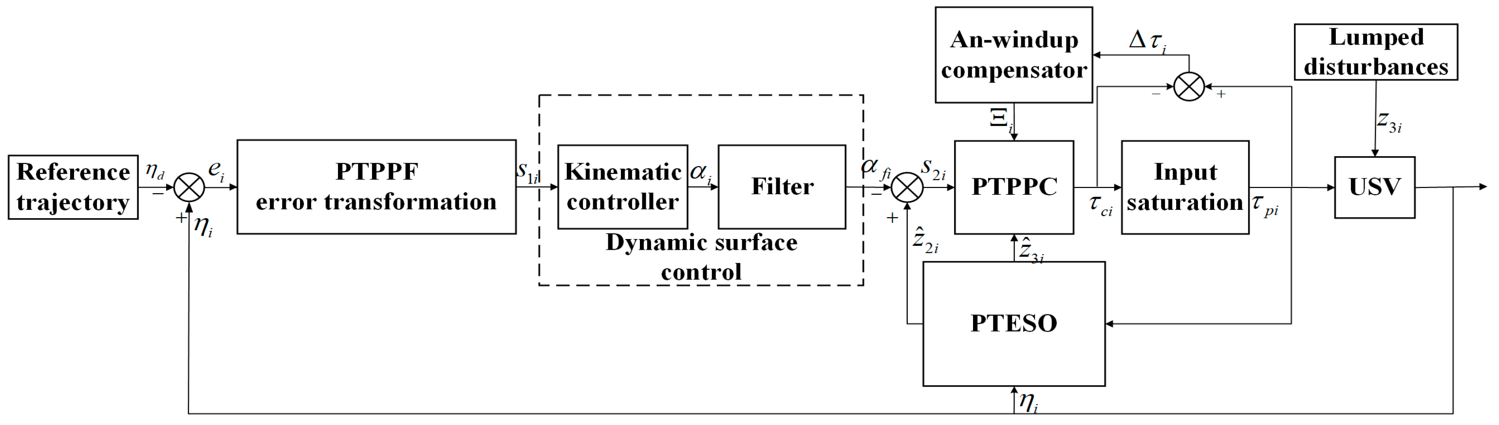
A suggested formation control strategy incorporates the observer, a prescribed performance technique, and a dynamic surface control algorithm. The designed approach guarantees accurate tracking control by allowing the formation tracking error to converge to a certain precision within a designated timeframe.

2. Preliminaries

2.1. Graph Theory

Suppose that a formation system of multiple USVs is composed of one leader USV and n follower USVs. A node is represented by each follower USV. A graph G = V , E with a collection of nodes V = 1 , 2 , , n and edges E = V × V is used to depict the communication across the formation system. If j is a neighbor of node i , then i , j E means that i th USV may receive the information sent by j th USV. N i = { j V | ( j , i ) E } represents the neighbor set of nodes i . The adjacency matrix A = a i , j R n × n associated with G is defined such that a i , j > 0 if ( i , j ) E , otherwise a i , j = 0 D = diag D 1 , D n R n × n is an in-degree matrix. Additionally, B = d i a g b 1 , , b n describes the communication interaction between n followers and leader. b i > 0 indicates i is able to obtain the information from leading USV; otherwise, b i = 0 .

2.2. USV Dynamics

Considering n underactuated USVs, the dynamics for the i th USV can be described as
η ˙ i = J i ( ψ i ) ν i M i ν ˙ i = τ c i + d i + g i
where η i = [ x , y , ψ ] T denotes the position vector ( x i , y i ) and the heading angle ψ i ; ν i = [ u i , v i , r i ] T denotes the velocity vector. J i ( ψ i ) is the rotation matrix, which is expressed as
J i ( ψ i ) = cos ( ψ i ) sin ( ψ i ) 0 sin ( ψ i ) cos ( ψ i ) 0 0 0 1
where g i = [ g u i , g v i , g r i ] T represents nonlinear dynamics with g u i ( u i , v i , r i ) = m 22 i v i r i d 11 i u i ; g v i ( u i , v i , r i ) = m 11 i u i r i d 22 i v i ; g r i ( u i , v i , r i ) = m 11 i m 22 i u i v i d 33 i r i , and M i = d i a g ( m 11 i , m 22 i , m 33 i ) is the inertial matrix, d 11 i , d 22 i and d 33 i are hydrodynamic coefficients. d i = [ d u i , d v i , d r i ] T is the external disturbances. τ c i = [ τ u i , 0 , τ r i ] T is the control input. The following equation describes the saturation limits
τ p i = s i g n ( τ c i ) τ M i , τ c i τ M i τ c i , τ c i < τ M i , i = u , r
where τ p i represents the actual control inputs. τ c i indicates the command control inputs. τ M i is the maximum value of saturation constraint.
To tackle the underactuation issue of unmanned surface vessels, the subsequent coordinate transformation is implemented,
η i = x i + L cos ( ψ i ) , y i + L sin ( ψ i ) T = x i , y i T
where L > 0 . Define ν i = [ u i , r i ] T , by deriving η i we have
η ˙ i = J i , 1 ν i + J i , 2 ( v i , ψ i ) ν ˙ i = M i 1 g i + τ i + d i
with J i , 1 = cos ( ψ i ) L sin ( ψ i ) sin ( ψ i ) L cos ( ψ i ) , J i , 2 = v i sin ( ψ i ) v i cos ( ψ i ) , M i = m 11 i 0 0 m 33 i , g i = g u i g r i , τ c i = τ u i τ r i , d i = d u i d r i .

2.3. Prescribed-Time Prescibed Performance Function (PTPPF)

The following performance constraint is developed to achieve the specified performance objectives,
λ 1 φ i ( t ) < z i ( t ) < λ 2 φ i ( t )
where z i ( t ) R 3 represents an auxiliary error. λ 1 and λ 2 are constants. φ i ( t ) is PTPPF function and its derivatives can be expressed as
φ ˙ i ( t ) = m + n γ ˙ φ γ φ φ i ( t ) φ i ( T f ) + ϑ i
where m and n are constants. φ ( T f ) is steady-state value of performance function. γ φ is constructed as
γ φ = T f h ( T f + t 0 t ) h ,   t [ t 0 , T f ) 1 , t [ T f , )
where T f is a user-defined time. ϑ is structured as
ϑ i = φ f ( m + n γ ˙ φ γ φ ) ( 1 ρ ( 1 cos ( π t T m ) ) ) , t [ 0 , T m ) φ f ( m + n γ ˙ φ γ φ ) ( 1 2 ρ ) ( 1 + cos ( π t π T m T f T m ) ) , t [ T m , T f ) 0 , t [ T f , )
where 0 < T m < T f , φ i f = φ ( 0 ) φ ( T f ) , ρ i = ρ i ρ i , γ ¯ φ = m n γ ˙ φ γ φ , k m = γ ¯ φ 2 + ( π T m ) 2 , k n = γ ¯ φ 2 + ( π T f T m ) 2 . Furthermore, ρ i and ρ i are designed as
ρ i = ( 1 2 γ ¯ φ γ ¯ φ 2 k n ) exp ( γ ¯ φ ( T f T m ) ) + 1 2 γ ¯ φ γ ¯ φ 2 k n
ρ i = ( γ ¯ φ k m 1 γ ¯ φ ) exp ( γ ¯ φ T f ) + ( 1 k m 1 k n ) exp ( γ ¯ φ ( T f T m ) ) + 1 γ ¯ φ γ ¯ φ k n

2.4. Lemma and Assumption

Initially, construct the subsequent time-varying function
γ ( t ) = T h ( T + t 0 t ) h , t [ t 0 , T ) 1 , t [ T , )
where T is the predefined time. Taking the derivative of γ ( t ) , we have
γ ˙ ( t ) = h T γ 1 + 1 h , t [ t 0 , T ) 0 , t [ T , )
Lemma 1 
([24]). For system x ˙ = p ( x ) + q ( x ) u , if there exists a continuous and differentiable Lyapunov function satisfying
V ˙ ( t ) k a ( t ) V ( t ) + a ( t ) Υ ( t )
where k R + , Υ ( t ) Υ ¯ , Υ ¯ R + . a ( t ) = T s / ( T s t ) satisfies a ( t ) : [ 0 , T s ) [ 1 , + ) , then the system is prescribed-time stable.
Assumption 1 
([25]). The external disturbances d i are bounded.
Assumption 2 
([26]).  η d = [ x d , y d , ψ d ] T is smooth and differentiable with bounded η ˙ d and η ¨ d .
Assumption 3 
([27]). The subsequent restriction is satisfied by the initial error
λ 1 φ i ( 0 ) < z i ( 0 ) < λ 2 φ i ( 0 )
Assumption 4 
([28]).  G has a spanning tree with the virtual leader being the root node.

3. Main Results

This research develops a prescribed-time prescribed performance control scheme (PTPPC) for underactuated multiple USV formation control, ensuring both the convergence accuracy and the convergence rate for the formation tracking errors. Figure 1 illustrates the schematic diagram of the designed control scheme.

3.1. Prescribed-Time Extended State Observer (PTESO)

Define an auxiliary vector ξ i = J i ( ψ i ) ν i = ξ i , 1 , ξ i , 2 , ξ i , 3 T , then Equation (1) can be transformed into
η ˙ i = ξ i ξ ˙ i = J i ( ψ i ) M i 1 τ p i + f i
where f i = [ f i , 1 , f i , 2 , f i , 3 ] = J i ( ψ i ) M i 1 ( g i + d i ) . Furthermore, let z 1 i = η i , z 2 i = η ˙ i , z 3 i = f i , and USV dynamics can be further described as
z ˙ 1 i = z 2 i z ˙ 2 i = z 3 i + J i ( ψ i ) M i 1 τ p i z ˙ 3 i = i ( t )
where i ( t ) is derivative of extended state.
Then, construct the following PTESO
z ^ ˙ 1 i = z ^ 2 i + k 1 χ i ( t ) ς i ( z 1 i z ^ 1 i ) z ^ ˙ 2 i = z ^ 3 i + J i ( ψ i ) M i 1 τ p i + k 2 χ i 2 ( t ) ς i 2 ( z 1 i z ^ 1 i ) z ^ ˙ 3 i = k 3 χ i 3 ( t ) ς i 3 ( z 1 i z ^ 1 i )
where z ^ 1 i , z ^ 2 i and z ^ 3 i denote the estimations of z 1 i , z 2 i and z 3 i , respectively. k 1 , k 2 and k 3 are observer gains. ς i denotes observer bandwidth. χ i ( t ) is a time-varying function
χ i ( t ) = T o + ϖ i T o + ϖ i t , 0 t < T o χ ¯ i , t T o
where χ ¯ i = 1 + T o / ϖ i , ϖ i R + . In the following content, for convenience, χ i ( t ) is represented as χ i .
Subsequently, design estimation errors z ˜ 1 i = z 1 i z ^ 1 i , z ˜ 2 i = z 2 i z ^ 2 i and z ˜ 3 i = z 3 i z ^ 3 i . By integrating (17) and (18), the subsequent error dynamics may be derived.
z ˜ ˙ 1 i = z ˜ 2 i k 1 χ i ς i z ˜ 1 i z ˜ ˙ 2 i = z ˜ 3 i k 2 χ i 2 ς i 2 z ˜ 1 i z ˜ ˙ 3 i = i ( t ) k 3 χ i 3 ς i 3 z ˜ 1 i
Additionally, by designing ϕ i = [ z ˜ 1 i T , χ i 1 ς i 1 z ˜ 2 i T , χ i 2 ς i 2 z ˜ 3 i T ] T , the vector representation of (20) is as follows:
ϕ ˙ i = χ i ς i P i I 3 ϕ + Q i I 3 i ( t ) / χ i 2 ς i 2 + Π i = χ i ς i P ¯ i ϕ i + Q ¯ i i ( t ) / χ i 2 ς i 2 + Π i
where Π i = χ i ϖ ¯ i ϕ i , ϖ ¯ i R 9 × 9 is a coefficient matrix. P ¯ i and Q ¯ i satisfy
P ¯ i = P i I 3 , Q ¯ i = Q i I 3 P i = [ k 1 , 1 , 0 ; k 2 , 0 , 1 ; k 3 , 0 , 0 ] Q i = [ 0 , 0 , 1 ]
According to (20), the transfer function between z ˜ 1 i and i ( t ) is
z ˜ 1 i L ( s ) i L 1 ( s ) = ( s 3 + k 1 χ i L 2 ( s ) ς i s 2 + k 2 χ i L 2 ( s ) ς i 2 s + k 3 χ i L 3 ( s ) ς i 3 ) 1
where x ˜ 1 i L ( s ) = L [ z ˜ 1 i ( t ) ] , which means z ˜ 1 i L ( s ) is obtained by the Laplace transformation of z ˜ 1 i ( t ) , so are i L ( s ) and χ i L ( s ) . To ensure P i is Hurwitz, choose the subsequent characteristic polynomial:
( s + χ i L ( s ) ς i ) 3 = s 3 + 3 χ i L ( s ) ς i s 2 + 3 χ 2 i L ( s ) ς i 2 s 1 + χ 3 i L ( s ) ς i 3
Therefore, it is reasonable that k 1 = k 2 = 3 and k 3 = 1 by combining (23) and (24).
Theorem 1.
For (17), based on Assumption 1, PTESO observer Equation (18) is designed and choose suitable gains k 1 , k 2 , k 3 , and χ i , so that the observer variables z 1 i , z 2 i , and z 3 i are accurately estimated within the predefined time T o .
Proof. 
By selecting suitable observer gains k 1 , k 2 , and k 3 such that P i is Hurwitz, then P ¯ i = P i I 3 is also Hurwitz, thus P ¯ i T A i + A i P ¯ i = I 9 holds, where I 9 R 9 × 9 is an identity matrix and A i R 9 × 9 is a positive definite matrix. Formulate the Lyapunov function as follows
V 0 = ϕ i T A i ϕ i
By integrating (21) and taking the derivative (25), we obtain
V ˙ 0 = ϕ ˙ i T A i ϕ i + ϕ i T A i ϕ ˙ i = χ i ς i ϕ i T P ¯ i T + i T ( t ) Q ¯ i T / χ i 2 ς i 2 + Π i T A i ϕ i + ϕ i T A i χ i ς i P ¯ i ϕ i + Q ¯ i i ( t ) / χ i 2 ς i 2 + Π i = χ i ς i ϕ i T ϕ i + 2 ϕ i T A i Q ¯ i i ( t ) / χ i 2 ς i 2 + A i Π i
Considering χ i [ 1 , 1 + T o / ϖ i ] and Yang’s inequality, we have
2 ϕ i T A i Q ¯ i i ( t ) / χ i 2 ς i 2 2 λ max A i ϕ i i ( t ) / ς i 2 ϕ i T ϕ i / χ i + χ i ε i 2 ϕ i T ϕ i + χ i ε i 2
where ε i = λ max A i ¯ i ( t ) / ς i 2 , i ( t ) < ¯ i , ¯ i R + ; λ max ( A i ) is the maximum eigenvalue of A i . Combining (27), (26) can be rephrased as
V ˙ 0 χ i ς i 2 λ max A i ϖ ¯ i ϕ i T ϕ i + ϕ i T ϕ i + χ i ε i 2 = χ i ς i 2 λ max A i ϖ ¯ i 1 ϕ i T ϕ i + χ i ε i 2 χ i K 0 V 0 + χ i Υ i
where K 0 = 2 ς i 2 λ max A i ϖ ¯ i 1 / λ max A i , Υ i = ε i 2 . Furthermore, ς i > 2 λ max A i ϖ ¯ i + 1 such that K 0 R + . In line with Lemma 1, the observation errors z ˜ 1 i , z ˜ 2 i and z ˜ 3 i satisfy
lim t T o z ˜ j i = Ω 0 ,   j = 1 , 2 , 3
The proof of Theorem 1 is complete. □

3.2. Controller Design and Stability Analysis

Initially, define the formation tracking errors e i , 1 = e 1 , x i , e 1 , y i T R 2 for i th USV
e i , 1 = j = 1 n a i , j η i η i , j + b i η i η i , d
where η i , d R 2 is designed as
η i , d = η d + J ( ψ d ) l i , d
where J ( ψ d ) = cos ( ψ d ) sin ( ψ d ) sin ( ψ d ) cos ( ψ d ) , l i , d = [ ρ i , d cos ( θ i , d ) , ρ i , d sin ( θ i , d ) ] T , and ψ d = a tan 2 ( y ˙ d , x ˙ d ) . Similarly, η i , j R 2 is designed according to η j = [ x j , y j ] T , J ( ψ j ) = cos ( ψ j ) sin ( ψ j ) sin ( ψ j ) cos ( ψ j ) , l i , j = ρ i , j cos ( θ i , j ) , ρ i , j sin ( θ i , j ) T .
Subsequently, define a time-varying function
γ i ( t ) = T h ( T + t 0 t ) h , t [ t 0 , T ) 1 , t [ T , )
where T is a user-defined time. Taking the derivative of Equation (32), we have
γ ˙ i ( t ) = h T γ i 1 + 1 h , t [ t 0 , T ) 0 , t [ T , )
To attain performance constraints and specified time convergence, the following auxiliary error vector is delineated.
μ i , 1 = k e + c e γ ˙ i γ i e i , 1
where k e and c e are positive constants.
Taking the derivative of Equation (34), we obtain
μ ˙ i , 1 = c e γ i γ ¨ i γ ˙ i 2 γ i 2 e i , 1 + k e + c e γ ˙ i γ i e ˙ i , 1
The subsequent intermediate vector is introduced to simplify the design of the formation controller:
μ i , 1 = λ 2 φ i t Γ i l i , ƛ
where ƛ = λ 1 λ 2 , Γ i l i , ƛ = e l i e l i e l i + ƛ 1 e l i is a monotonically increasing function.
By solving Γ i l i , ƛ , we obtain
l i = 1 2 ln λ 1 φ i + μ i , 1 1 2 ln λ 2 φ i μ i , 1
Then, define the following transformation errors
s i , 1 = l i 1 2 ln λ 1 λ 2
Calculating the derivative of (38), we have
s ˙ i , 1 = i μ ˙ i , 1 μ i , 1 φ ˙ i φ i 1
where i = 1 2 μ i , 1 + λ 1 φ i 1 2 μ i , 1 λ 2 φ i .
Choose the subsequent Lyapunov function
V i , 1 = 1 2 s i , 1 T s i , 1
Combined with the derivative of V i , 1 and Equation (39), we obtain
V ˙ i , 1 = s i , 1 T i μ ˙ i , 1 μ i , 1 φ ˙ i φ i 1
According to (30) and (34), design the following virtual control law
α i = 1 b i ζ i , e μ i , 1 φ ˙ i φ i 1 i 1 N i , 1 s i , 1 c e φ i φ ¨ i φ ˙ i 2 φ i 2 e i , 1 + ζ e j N i a i j ξ j + ζ e b i η d
where N i , 1 are positive definite matrix; ζ i , e = k e + c e φ ˙ i φ i .
Then, the velocity tracking errors is defined
s i , 2 = ν i α i , f
To reduce the computational complexity, the following first-order filter is introduced
ι α ˙ i , f + α i , f = α i ,   α i , f ( 0 ) = α i ( 0 )
where ι is filtering constant; α i , f are filter output.
Then, the filtering errors are defined
σ i = α i , f α i
The calculation of the derivative of (45) proceeds in the following manner:
σ ˙ i = 1 ι σ i α ˙ i
Next, the derivative of Equation (43) can be calculated
s ˙ i , 2 = 1 / m 11 i τ u i + f ^ i , 1 cos ( ψ i ) + f ^ i , 2 sin ( ψ i ) + r i v ^ i + 1 / m 33 i τ r i + f ^ i , 3 α ˙ i , f
In addition, to solve the issue of input saturation, the following anti-saturation compensator is introduced
Ξ ˙ i = K i , Ξ Ξ i + Δ τ i
where K i , Ξ are positive matrix; Ξ i are the state vector of compensator.
Define F i = f ^ i , 1 cos ( ψ i ) + f ^ i , 2 sin ( ψ i ) , f ^ i , 3 T , ω i 1 = d i a g 1 ω i , u , 1 ω i , r , the following prescribed-time formation controller is designed
τ i , p = ω i 1 M i N i , 2 s i , 2 + α ˙ i , f F i + κ i , 3 Ξ i
where N i , 2 are positive definite matrix. f ^ i is the estimations of lumped disturbances.
Theorem 2.
Considering the lumped disturbances and input saturation constraints of the underactuated USV formation tracking control system (5), under the condition of satisfying Assumptions 1–4, combined with the proposed PTESO observer (18), kinematic controller (42), dynamic controller (49), and anti-saturation compensator (48), a formation tracking control scheme is proposed to ensure that the formation tracking error converges to the predefined range within the prescribed time T .
Proof. 
Define the following Lyapunov function
V i , 2 = 1 2 s i , 1 T s i , 1 + 1 2 s i , 2 T s i , 2 + 1 2 Ξ i T Ξ i + 1 2 σ i T σ i
The derivative of V i , 2 is
V ˙ i , 2 = s i , 1 T s ˙ i , 1 + s i , 2 T s ˙ i , 2 + Ξ i T Ξ ˙ i + σ i T σ ˙ i
According to (39), (43) and (44), we obtain
s i , 1 T s ˙ i , 1 = s i , 1 T i ( μ ˙ i , 1 μ i , 1 φ ˙ φ 1 ) = s i , 1 T i c e ( γ i γ ¨ i γ ˙ i 2 ) γ i 2 e i + ( k e + c e γ ˙ i γ i ) ( ν i η ˙ d ) μ i , 1 φ ˙ i φ i 1 = s i , 1 T i c e ( γ i γ ¨ i γ ˙ i 2 ) γ i 2 e i + ( k e + c e γ ˙ i γ i ) ( s i , 2 + σ i + α i η ˙ d ) μ i , 1 φ ˙ i φ i 1
Then, substituting (30) and (42) into (52), we obtain
s i , 1 T s ˙ i , 1 = s i , 1 T i k e + c e γ ˙ i γ i s i , 2 + σ i κ i , 1 s i , 1 = i k e + c e γ ˙ i γ i s i , 1 T s i , 2 + i k e + c e γ ˙ i γ i s i , 1 T σ i κ i , 1 s i , 1 T s i , 1
Combined with Young’s inequality, we have
s i , 1 T s ˙ i , 1 = i k e + c e γ ˙ i γ i s i , 1 T s i , 2 + i k e + c e γ ˙ i γ i s i , 1 T σ i κ i , 1 s i , 1 T s i , 1 i k e + c e γ ˙ i γ i ( 1 2 s i , 1 T s i , 1 + 1 2 s i , 2 T s i , 2 ) + i k e + c e γ ˙ i γ i ( 1 2 s i , 1 T s i , 1 + 1 2 σ i T σ i ) κ i , 1 s i , 1 T s i , 1 κ i , 1 i k e + c e γ ˙ i γ i s i , 1 T s i , 1 + 1 2 i k e + c e γ ˙ i γ i s i , 2 T s i , 2 + 1 2 i k e + c e γ ˙ i γ i σ i T σ i
Furthermore, from (46) and (48), we have
σ i T σ ˙ i = σ i T 1 ι σ i α ˙ i
Ξ i T Ξ ˙ i = Ξ i T K Ξ Ξ i + Δ τ i
Combining (54)–(56), (50) can be rewritten as
V ˙ i , 2 κ i , 1 i k e + c e γ ˙ i γ i s i , 1 T s i , 1 + 1 2 i k e + c e γ ˙ i γ i s i , 2 T s i , 2 + 1 2 i k e + c e γ ˙ i γ i σ i T σ i 1 ι σ i T σ i + σ i T α ˙ i Ξ i T K i , Ξ Ξ i + Ξ i T Δ τ i κ i , 2 s i , 2 T s i , 2
From Young’s inequality, we obtain
σ i T α ˙ i a i σ i T σ i + N i 2 4 a i
Then, substituting (58) into (57) yields
V ˙ i , 2 κ i , 1 i k e + c e γ ˙ i γ i s i , 1 T s i , 1 κ i , 2 1 2 i k e + c e γ ˙ i γ i s i , 2 T s i , 2 + 1 2 i k e + c e γ ˙ i γ i σ i T σ i 1 ι σ i T σ i + a 1 σ i T σ i + N i 2 4 a i Ξ i T K i , Ξ Ξ i + Ξ i T Δ τ i
Let k i , Ξ = λ min ( K i , Ξ ) and combine Young’s inequality
V ˙ i , 2 κ i , 1 i k e + c e γ ˙ i γ i s i , 1 T s i , 1 κ i , 2 1 2 i k e + c e γ ˙ i γ i s i , 2 T s i , 2 1 ι 1 2 i a i k e + c e γ ˙ i γ i σ i T σ i k i , Ξ 1 2 Ξ i 2 + 1 2 Δ τ i 2 + N i 2 4 a i
By selecting appropriate parameters, Φ i , 1 = κ i , 1 i k e + c e γ ˙ i γ i > 0 , Φ i , 2 = κ i , 2 1 2 i k e + c e γ ˙ i γ i > 0 , Φ i , 3 = 1 ι 1 2 i a i k e + c e γ ˙ i γ i > 0 , Φ i , 4 = k i , Ξ 1 2 > 0 .
From the above analysis, we can deduce that
V ˙ i , 2 2 δ i V i , 2 + Ω i
where δ i = min Φ i , 1 , Φ i , 2 , Φ i , 3 , Φ i , 4 ; Ω i = 1 2 Δ τ i 2 + N i 2 4 a i . By selecting appropriate parameters such that δ i > Ω i 2 p i and V i , 2 < p i are invariant sets, i.e., when V i , 2 ( 0 ) p i has V i , 2 ( t ) p i for any t 0 .
Furthermore, solving (61) yields
V i , 2 ( t ) e 2 δ i t V ( 0 ) + Ω i 2 δ i 1 e 2 δ i t
Based on the above discussion, it can be concluded that all signals in a closed-loop system are uniformly ultimately bounded (UUB).
According to (32) and (34), we have
e i , 1 = k e + c e γ ˙ i γ i 1 μ i , 1 < φ i ( T + t 0 t ) k e ( T + t 0 t ) + c e h i , t [ t 0 , T ) φ i k e , t [ T , )
From Equation (63), tracking errors e i , 1 can converge to the prescribed performance constrain e i , 1 < φ i k e within the prescribed time T .□

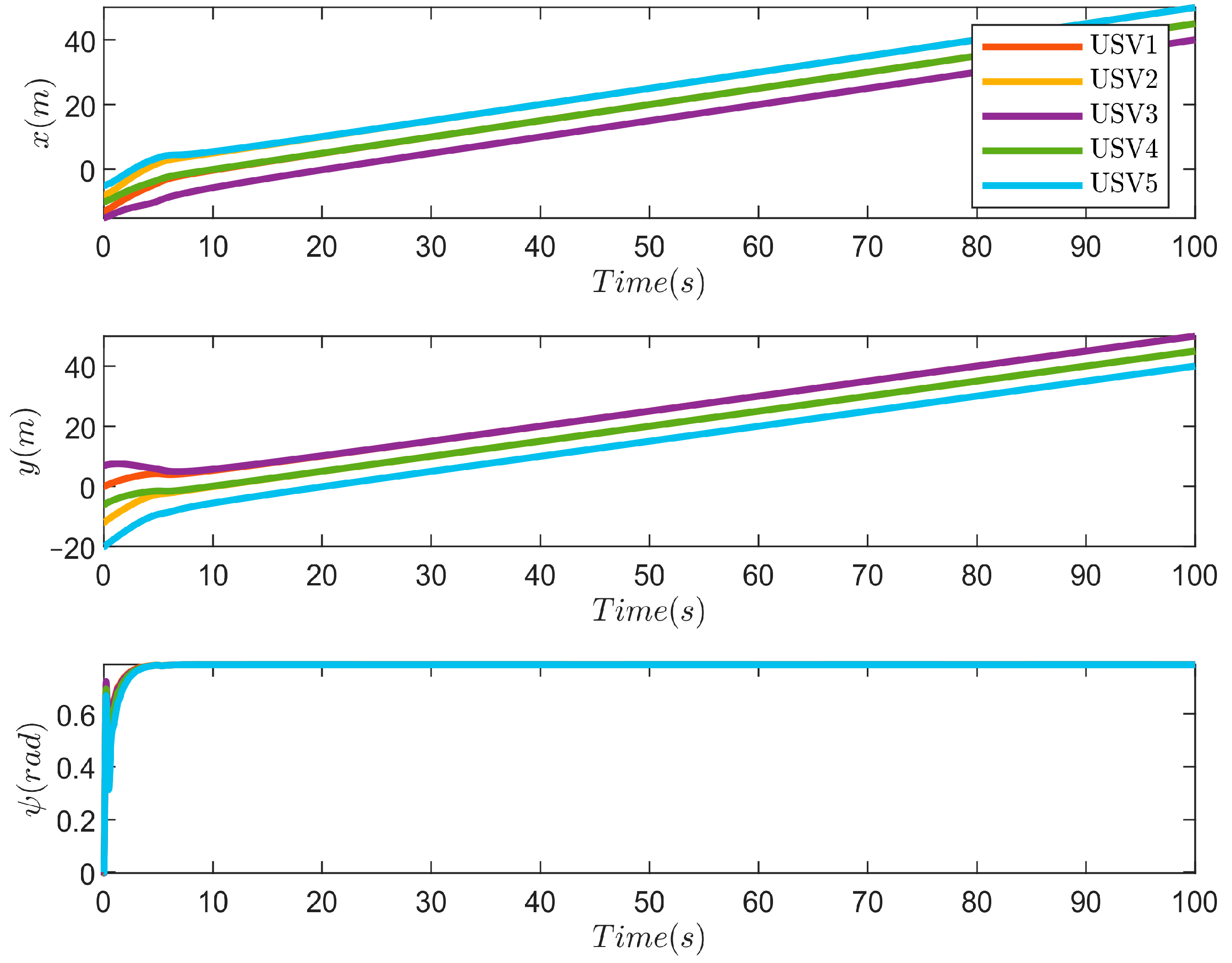
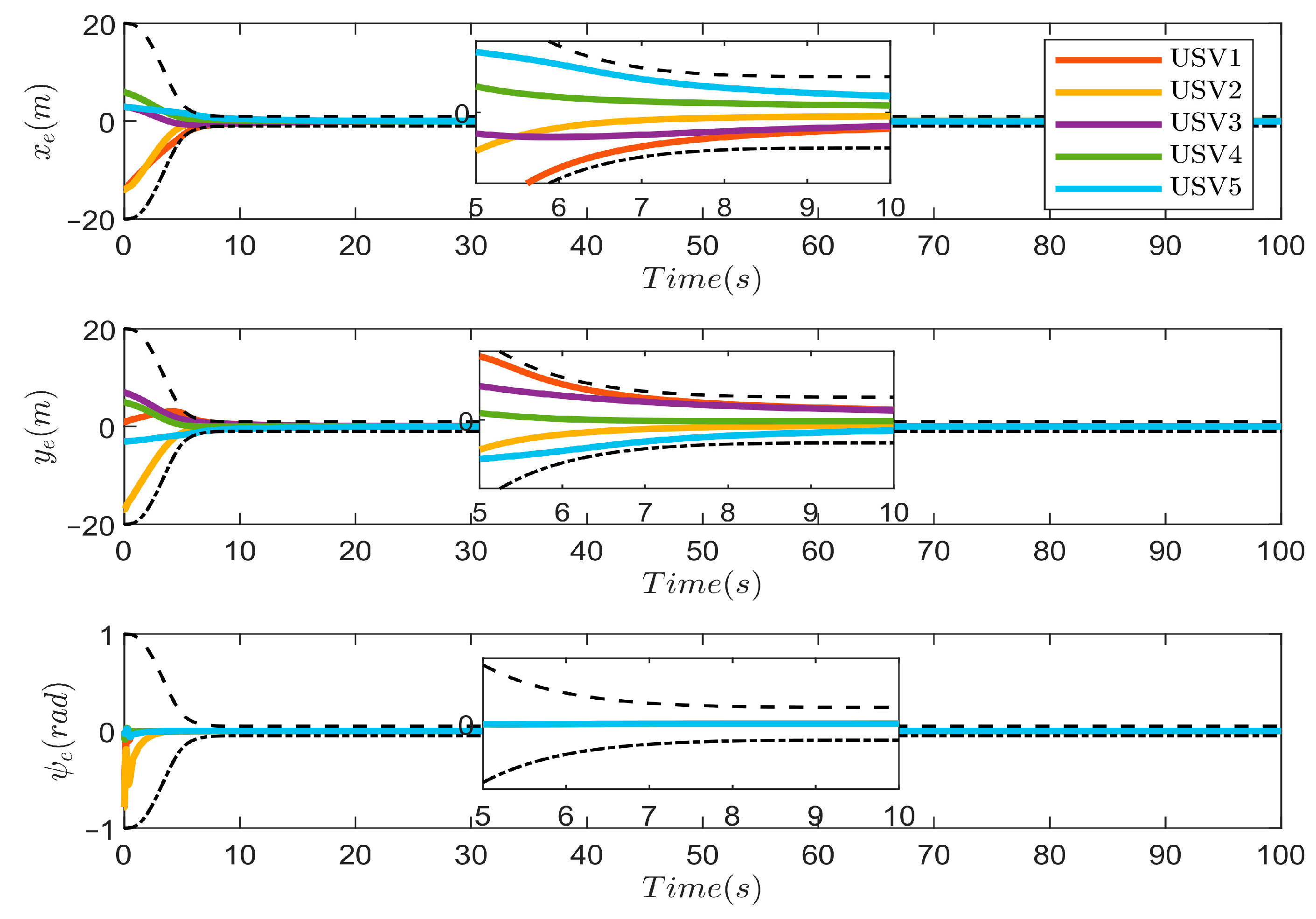
4. Simulation Results

To verify the effectiveness and superiority of the USV formation tracking control scheme proposed in this article, this paper takes Cybership II, developed by Norwegian University of Science and Technology, as the simulation object to verify the proposed formation tracking controller, and gives the result analysis. Detailed USV model parameters reference [29]. The formation parameters are set as ρ 1 , d = 5 2 , θ 1 , d = 0.75 π , ρ 2 , d = 5 2 , θ 2 , d = 0.75 π , ρ 3 , d = 10 2 , θ 3 , d = 0.75 π , ρ 4 , d = 10 , θ 4 , d = π , ρ 5 , d = 10 2 , θ 5 , d = 0.75 π . The desired trajectory η d of the leader USV is selected as follows
x d = 0.5 t y d = 0.5 t ψ d = a tan 2 ( y ˙ d , x ˙ d )
The external disturbances are set as
d u = 10 cos ( 0.15 t ) + 5 sin ( 0.3 t ) d v = 6 sin ( 0.25 t ) + 8 cos ( 0.2 t ) d r = 7 sin ( 0.35 t ) + 6 cos ( 0.1 t )
The initial states of USVs are selected as η 1 = [ 13 , 0 , 0 ] T , ν 1 = [ 0 , 0 , 0 ] T , η 2 = [ 8 , 12 , 0 ] T , ν 2 = [ 0 , 0 , 0 ] T , η 3 = [ 15 , 7 , 0 ] T , ν 3 = [ 0 , 0 , 0 ] T , η 4 = [ 10 , 6 , 0 ] T , ν 4 = [ 0 , 0 , 0 ] T , η 5 = [ 5 , 20 , 0 ] T , ν 5 = [ 0 , 0 , 0 ] T . The control parameters for the following USVs are k e = 1 , c e = 5 , N 1 i = d i a g ( 5 , 2 ) , N 2 i = d i a g ( 5 , 5 ) , ω i , u = ω i , r = 0.8 , T = 10   s . The parameters of prescribed performance are m = 1, n = 2, φ ( 0 ) = [ 20 , 20 , 1 ] T , φ ( T f ) = [ 1 , 1 , 0.05 ] T , Tf = 10, Tm = 5. The parameters of PTESO are given as k1 = 3, k2 = 5.5, k3 = 7, ς = 4, To = 5 s. The control input limits are designated as follows: τ u i [ 500 , 500 ] N , τ u i [ 200 , 200 ] N · m .
Figure 2 illustrates the communication topology among USVs. Figure 3 gives the trajectories of USV formation. It is evident that the five following USVs have effectively established and sustained the formation within the designated timeframe T = 10   s . The following USV positions and heading angles are shown in Figure 4. Figure 5 gives the formation tracking errors of the following USVs. According to Figure 5, the formation tracking errors can converge to preset range within the predefined time T = 10   s and always remain within the performance boundary. Figure 6 illustrates the control inputs of follower USVs. Under the action of the anti-saturation compensator, the control inputs are always within the predefined saturation constraints. Figure 7 and Figure 8, respectively, give the estimated values of the velocity and lumped disturbances with the proposed PTESO observer. It can be seen from the Figure 7 and Figure 8 that the observer can quickly estimate and compensate the system within the prescribed time T o = 5   s and improve the anti-interference ability of the system.
To fully verify the effectiveness and superiority of the proposed control scheme, it is compared with the USV formation control scheme based on disturbance observer in [30]. In addition, the proposed PTESO in this paper is compared with the finite-time extended state observer (FTESO) in [31] and the fixed-time extended state observer (FXESO) in [32]. The comparative simulation results are shown in Figure 9, Figure 10, Figure 11, Figure 12, Figure 13, Figure 14 and Figure 15. According to Figure 9, it can be seen that under the comparative control algorithm in [30], the USV trajectory exhibits oscillations during the initial formation stage, which will result in significant tracking errors. Figure 10 shows the position and heading curves of follower USVs. Figure 11 shows the formation tracking error curve under the comparative control algorithm in [30]. From Figure 11, under the action of the comparative control algorithm in [30], the heading tracking error cannot quickly converge to preset range within the prescribed time. In addition, according to Figure 12, the comparative control algorithm in [30] has a larger control input, resulting in more energy consumption. Figure 13 and Figure 14 show the velocity and lumped disturbance estimation curves under three kinds of observers, respectively. It can be seen that the proposed PTESO observer in this article has a faster convergence rate and accuracy, and the convergence time can be predefined regardless of the initial conditions. In addition, to quantify the control performance of the formation control scheme, the following comprehensive performance indicators (CPI) are defined
C P I = i = 1 5 e i , 1 2 1 / 2
The CPI values of the control algorithm in this paper and the control algorithm in [30] are shown in Figure 15. Compared with the comparison algorithm, the CPI value of the control algorithm proposed in this paper is smaller and has a faster convergence rate. This feature indicates that the control algorithm proposed in this paper has higher performance in terms of convergence rate and tracking accuracy. On the other hand, 0 t τ p i T ( s ) τ p i ( s ) 1 / 2 d s   ( i = 1 , 2 , 3 , 4 ) is used to quantitatively evaluate the energy consumption for each following USV. As shown in Figure 16, the energy consumption of the controller proposed in this paper is significantly lower than that of the comparison controller, thus showing high economic value and practicality.

5. Conclusions

This research studies a prescribed-time formation tracking control scheme for multiple underactuated USVs. A PTESO is used to estimate the unmeasured velocities and lumped disturbances. A PTPPF function is designed to achieve guaranteed performance. The formation controller is proposed by employing prescribed-time theory, prescribed performance constraints, and dynamic surface control. Ultimately, the Lyapunov stability theory analysis demonstrated that all signals in the control system are bounded and tracking errors exhibit prescribed-time stability. Comparative simulations showed that even with unknown velocities, the suggested technique may produce fewer steady state errors and quicker convergence. Nevertheless, the suggested control scheme permits multiple USVs to achieve formation within a certain timeframe; however, it does not provide active obstacle avoidance. Consequently, further research will concentrate on the formation control of multiple underactuated USVs, including anti-collision and obstacle avoidance characteristics to address the intricacies and variety of practical navigation situations.

Author Contributions

Methodology, B.S.; Software, B.S. and J.Z.; Validation, B.S.; Investigation, B.S.; Writing—original draft, B.S.; Writing—review & editing, J.Z.; Supervision, J.Z. and Z.L.; Project administration, Z.L. All authors have read and agreed to the published version of the manuscript.

Funding

This research was funded by the National Natural Science Foundation of China, grant number 62473373.

Institutional Review Board Statement

Not applicable.

Informed Consent Statement

Not applicable.

Data Availability Statement

The original contributions presented in the study are included in the article; further inquiries can be directed to the corresponding author.

Conflicts of Interest

The authors declare no conflicts of interest.

Abbreviations

The following symbols are used in this manuscript:
G 
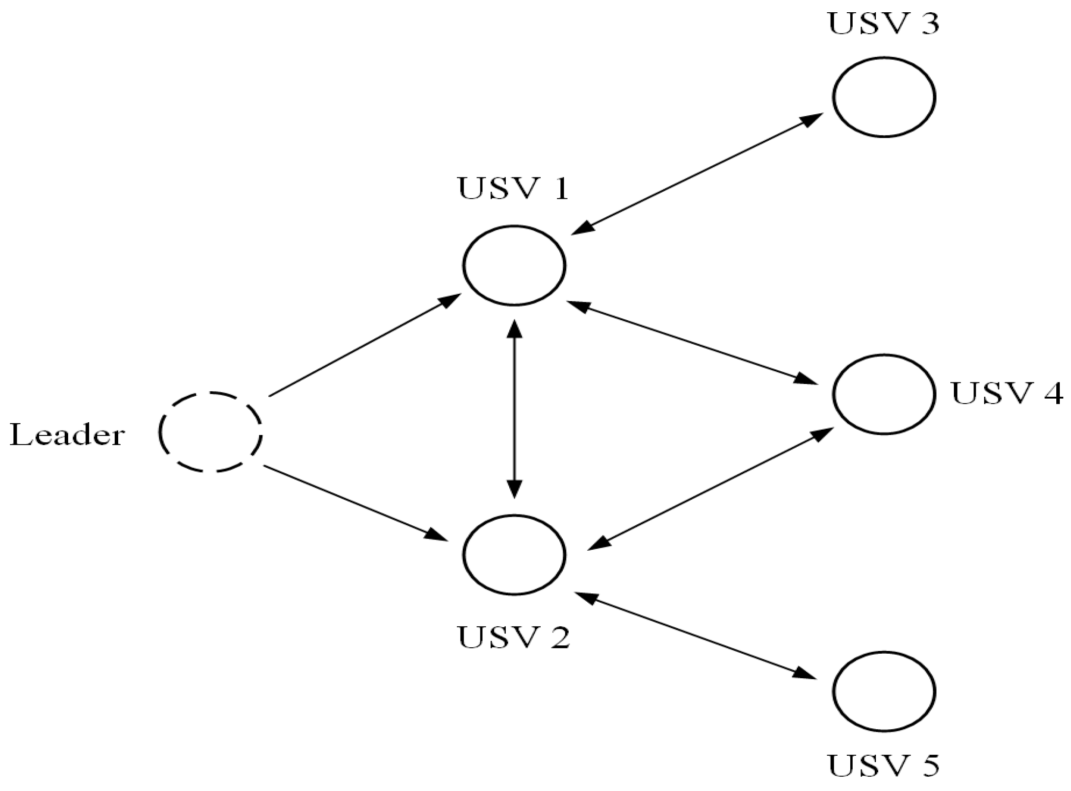
The communication topology diagram.
V The node of communication topology graph.
E The edge of communication topology graph.
N i The set of neighbors of the i th node.
A The adjacency matrix.
D The in-degree matrix.
L The Laplacian matrix.
B The incidence matrix.
J The rotation matrix.
M The inertial matrix.
φ The prescribed performance function
γ The nonlinear time-varying function.
z ^ i The observations of state observer.
σ The filtering error.
α i The kinematics control law.
τ i , p The dynamics control law.
Ξ The state of compensator.

References

  1. Chen, C.; Zou, W.; Xiang, Z. Event-Triggered Connectivity-Preserving Formation Control of Heterogeneous Multiple USVs. IEEE Trans. Syst. Man Cybern. Syst. 2024, 54, 7746–7755. [Google Scholar] [CrossRef]
  2. Fan, Y.; Li, Z.; Li, J.; Ma, G.; Bu, H. Fixed-time event-triggered distributed formation control for underactuated USVs considering actuator saturation. Ocean Eng. 2025, 316, 119829. [Google Scholar] [CrossRef]
  3. Wu, T.; Xue, K.; Wang, P. Leader-follower formation control of USVs using APF-based adaptive fuzzy logic nonsingular terminal sliding mode control method. J. Mech. Sci. Technol. 2022, 36, 2007–2018. [Google Scholar] [CrossRef]
  4. Chen, C.; Liao, Y.; Tang, X.; Sun, J.; Gu, J.; Li, H.; Ren, Z.; Zhai, Z.; Li, Y.; Wang, B.; et al. Research on double-USVs fuzzy-priority NSB behavior fusion formation control method for oil spill recovery. J. Field Robot. 2025, 42, 302–326. [Google Scholar] [CrossRef]
  5. Jiang, X.; Xia, G. Sliding mode formation control of leaderless unmanned surface vehicles with environmental disturbances. Ocean Eng. 2022, 244, 110301. [Google Scholar] [CrossRef]
  6. Fang, X.; Wen, G.; Yu, X.; Chen, G. Formation control for unmanned surface vessels: A game-theoretic approach. Asian J. Control 2022, 24, 498–509. [Google Scholar] [CrossRef]
  7. Tan, G.; Zhuang, J.; Zou, J.; Wan, L. Coordination control for multiple unmanned surface vehicles using hybrid behavior-based method. Ocean Eng. 2021, 232, 109147. [Google Scholar] [CrossRef]
  8. Fan, J.; Liao, Y.; Li, Y.; Jiang, Q.; Wang, L.; Jiang, W. Formation control of multiple unmanned surface vehicles using the adaptive null-space-based behavioral method. IEEE Access 2019, 7, 87647–87657. [Google Scholar] [CrossRef]
  9. Zhang, G.; Yu, W.; Li, J.; Zhang, X. A novel event-triggered robust neural formation control for USVs with the optimized leader–follower structure. Ocean Eng. 2021, 235, 109390. [Google Scholar] [CrossRef]
  10. Xie, M.; Wu, Z.; Huang, H. Low-complexity formation control of marine vehicle system based on prescribed performance. Nonlinear Dyn. 2024, 112, 18311–18332. [Google Scholar] [CrossRef]
  11. Liu, G.; Wen, N.; Long, F.; Zhang, R. A Formation Control and Obstacle Avoidance Method for Multiple Unmanned Surface Vehicles. J. Mar. Sci. Eng. 2023, 11, 2346. [Google Scholar] [CrossRef]
  12. Zhen, Q.; Wan, L.; Li, Y.; Jiang, D. Formation control of a multi-AUVs system based on virtual structure and artificial potential field on SE(3). Ocean Eng. 2022, 253, 111148. [Google Scholar] [CrossRef]
  13. Liu, C.; Wang, Y. Neural adaptive performance guaranteed formation control for USVs with event-triggered quantized inputs. Ships Offshore Struct. 2024, 1–13. [Google Scholar] [CrossRef]
  14. Xia, G.; Xia, X.; Zheng, Z. Formation tracking control for underactuated surface vehicles with actuator magnitude and rate saturations. Ocean Eng. 2022, 260, 111935. [Google Scholar] [CrossRef]
  15. Sun, Z.; Sun, H.; Li, P.; Zou, J. Formation control of multiple underactuated surface vessels with a disturbance observer. J. Mar. Sci. Eng. 2022, 10, 1016. [Google Scholar] [CrossRef]
  16. Ma, Y.; Ning, J.; Li, T.; Liu, L. Distributed extended state observer-based formation tracking control of under-actuated unmanned surface vehicles with input and state quantization. Ocean Eng. 2024, 311, 118872. [Google Scholar] [CrossRef]
  17. Dong, Z.; Zhang, Z.; Qi, S.; Zhang, H.; Li, J.; Liu, Y. Autonomous cooperative formation control of underactuated USVs based on improved MPC in complex ocean environment. Ocean Eng. 2023, 270, 113633. [Google Scholar] [CrossRef]
  18. Dong, C.; Ye, Q.; Dai, S.L. Neural-network-based adaptive output-feedback formation tracking control of USVs under collision avoidance and connectivity maintenance constraints. Neurocomputing 2020, 401, 101–112. [Google Scholar] [CrossRef]
  19. Peng, H.; Huang, B.; Jin, M.; Zhu, C.; Zhuang, J. Distributed finite-time bearing-based formation control for underactuated surface vessels with Levant differentiator. ISA Trans. 2024, 147, 239–251. [Google Scholar] [CrossRef]
  20. Jiang, Y.; Liu, Z.; Chen, F. Adaptive output-constrained finite-time formation control for multiple unmanned surface vessels with directed communication topology. Ocean Eng. 2024, 292, 116552. [Google Scholar] [CrossRef]
  21. Wu, W.; Tong, S. Fixed-time formation fault tolerant control for unmanned surface vehicle systems with intermittent actuator faults. Ocean Eng. 2023, 281, 114813. [Google Scholar] [CrossRef]
  22. An, S.; Liu, Y.; Wang, X.; Fan, Z.; Zhang, Q.; He, Y.; Wang, L. Distributed Event-Triggered Fixed-Time Leader–Follower Formation Tracking Control of Multiple Underwater Vehicles Based on an Adaptive Fixed-Time Observer. J. Mar. Sci. Eng. 2023, 11, 1522. [Google Scholar] [CrossRef]
  23. Song, Y.; Wang, Y.; Holloway, J.; Krstic, M. Time-varying feedback for regulation of normal-form nonlinear systems in prescribed finite time. Automatica 2017, 83, 243–251. [Google Scholar] [CrossRef]
  24. Li, J.; Song, S. Prescribed-time collision-free trajectory tracking control for spacecraft with position-only measurements. IEEE Trans. Aerosp. Electron. Syst. 2024, 60, 4035–4043. [Google Scholar] [CrossRef]
  25. Wu, G.X.; Ding, Y.; Tahsin, T.; Atilla, I. Adaptive neural network and extended state observer-based non-singular terminal sliding mode tracking control for an underactuated USV with unknown uncertainties. Appl. Ocean Res. 2023, 135, 103560. [Google Scholar] [CrossRef]
  26. Shen, Z.; Wang, Q.; Dong, S.; Yu, H. Dynamic surface control for tracking of unmanned surface vessel with prescribed performance and asymmetric time-varying full state constraints. Ocean Eng. 2022, 253, 111319. [Google Scholar] [CrossRef]
  27. Sui, B.; Zhang, J.; Liu, Z. Extended state observer based prescribed-time trajectory tracking control for USV with prescribed performance constraints and input saturation. Ocean Eng. 2025, 316, 120005. [Google Scholar] [CrossRef]
  28. Li, J.; Fan, Y.; Liu, J. Distributed fixed-time formation tracking control for multiple underactuated USVs with lumped uncertainties and input saturation. ISA Trans. 2024, 154, 186–198. [Google Scholar] [CrossRef]
  29. Skjetne, R.; Fossen, T.I.; Kokotović, P.V. Adaptive maneuvering, with experiments, for a model ship in a marine control laboratory. Automatica 2005, 41, 289–298. [Google Scholar] [CrossRef]
  30. Li, J.; Fu, M.; Wang, L. Formation control for underactuated surface vehicles in the presence of ocean current. In Proceedings of the OCEANS 2022, Hampton Roads, VA, USA, 17–20 October 2022; IEEE: Piscataway, NJ, USA, 2022; pp. 1–7. [Google Scholar]
  31. Fu, M.; Yu, L. Finite-time extended state observer-based distributed formation control for marine surface vehicles with input saturation and disturbances. Ocean Eng. 2018, 159, 219–227. [Google Scholar] [CrossRef]
  32. Wang, T.; Liu, Y.; Zhang, X. Extended state observer-based fixed-time trajectory tracking control of autonomous surface vessels with uncertainties and output constraints. ISA Trans. 2022, 128, 174–183. [Google Scholar] [CrossRef]
Figure 1. The schematic diagram of the proposed control scheme.
Jmse 13 00480 g001
Figure 2. The communication topology graph.
Jmse 13 00480 g002
Figure 3. Trajectories of USV formation.
Jmse 13 00480 g003
Figure 4. The position and heading of follower USVs.
Jmse 13 00480 g004
Figure 5. The USV formation tracking errors.
Jmse 13 00480 g005
Figure 6. The control inputs of follower USVs.
Jmse 13 00480 g006
Figure 7. The velocity estimation of the PTESO observer.
Jmse 13 00480 g007
Figure 8. The lumped disturbance estimations of the PTESO observer.
Jmse 13 00480 g008
Figure 9. Trajectories of USV formation under the control algorithm in [30].
Jmse 13 00480 g009
Figure 10. The position and heading of follower USVs under the control algorithm in [30].
Jmse 13 00480 g010
Figure 11. The USV formation tracking errors under the control algorithm in [30].
Jmse 13 00480 g011
Figure 12. The control inputs of follower USVs under the control algorithm in [30].
Jmse 13 00480 g012
Figure 13. The velocity estimations of different observers.
Jmse 13 00480 g013
Figure 14. The lumped disturbance estimations of different observers.
Jmse 13 00480 g014
Figure 15. The CPI values of two kinds of control schemes.
Jmse 13 00480 g015
Figure 16. The energy consumption of two kinds of control schemes.
Jmse 13 00480 g016
Disclaimer/Publisher’s Note: The statements, opinions and data contained in all publications are solely those of the individual author(s) and contributor(s) and not of MDPI and/or the editor(s). MDPI and/or the editor(s) disclaim responsibility for any injury to people or property resulting from any ideas, methods, instructions or products referred to in the content.

