Research on a Fully Parameterized Geometric Modeling Method for an Air Cavity Planing Hull

Abstract

An air-lubricated planing hull with integrated air channels presents a transformative approach for enhancing marine vessel performance by significantly reducing hydrodynamic resistance. Within the framework of air-layer drag reduction research, the precise definition and optimization of geometric design parameters are critical, as they directly influence the formation and stability of the air layer and the hydrodynamic characteristics of the hull. Applying a fully parameterized modeling approach to the air-lubricated planing hull is highly relevant and pivotal for advancing systematic, performance-driven hull design and optimization in modern naval architecture. This study proposes a fully parameterized modeling method specifically designed for such crafts. The method utilizes B-spline curves to represent the planar projections of the primary hull contours and the sectional lines of key hull surfaces. The hull surfaces are fitted using non-uniform rational B-Spline (NURBS) surfaces, and the design parameters are smoothed according to the principle of minimum strain energy, leading to fair and smooth hull surfaces. A dedicated program is developed based on this method. It facilitates the rapid generation of smooth hull forms for an air-lubricated planing hull solely from design parameters without depending on parent hull forms. This approach provides geometric hull samples for optimizing the hydrodynamic performance of the air-lubricated planing hull.

1. Introduction

During navigation, a ship is primarily influenced by three types of resistance: frictional resistance, viscous pressure resistance, and wave-making resistance. Injecting air beneath the hull during transit creates a uniform and stable gas–liquid two-phase flow. This approach effectively reduces the ship’s resistance by leveraging the differences in density and viscosity between water and air. Air lubrication drag reduction technology has long been of interest to researchers [1].

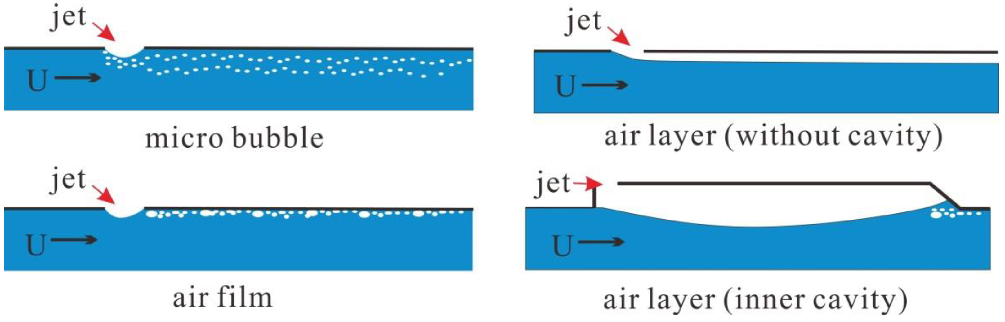
As illustrated in Figure 1, the methods of air lubrication drag reduction can be categorized into two main types based on their mechanisms and gas distribution forms: bubble drag reduction (BDR) and air-layer drag reduction (ALDR). BDR encompasses various techniques, including microbubble drag reduction, bubble drag reduction, transitional air-layer drag reduction, and air curtain drag reduction. A defining characteristic of BDR is the mixing of gas and liquid without a distinct interface, which typically requires minimal modifications to the hydrodynamic shape of the hull. The majority of vessels using the BDR technology do not need to set up extra cavity structures.

Elbing et al. [2] investigated the transition relationships between bubble, transitional, and air-layer drag reductions, revealing that at higher airflow rates, the drag reduction mechanism shifts to ALDR, which offers greater efficiency.

A hull bottom, designed with a proper cavity, can facilitate the development of a stable air layer. Typically, air cavities are introduced at the bottom of the hull to facilitate the generation of an air layer. In contrast, the sidewalls of these cavities help prevent airflow from escaping along the sides of the hull, thereby maintaining the stability of the air layer. This method, which employs air cavities for drag reduction in the air layer, is referred to by some researchers as partial cavity drag reduction (PCDR) or air cavity drag reduction (ACDR) [3,4]. Implementing this approach usually necessitates modifying the hull shape by adding cavity structures at its base.

As early as 1968, Butuzov [5] conducted theoretical studies on flat-plate air cavities. After 2000, many researchers began investigating the application of air-layer drag reduction (ALDR) technology for high-speed hulls. Matveev et al. [6,7] conducted experimental studies on air injection drag reduction and cavity length using a simplified flat-bottom ship model measuring 0.56 m long and featuring longitudinal grooves on its bottom. Their findings showed good agreement between the linear potential flow theoretical model and experimental results, indicating that hull geometry changes significantly influence the air-layer distribution. In 2022, Matveev [8] carried out research on the air cavity system of a planing hull with two steps in the bottom. Computational fluid dynamics was used to model an air cavity system. Simulations of the modified hull at various speeds and center of gravity positions were conducted, obtaining data on resistance, trim, heave, and air cavity shapes, and a favorable loading condition was identified. Shallow water simulation studies showed that in the steady state, the performance drops significantly near the critical speed, while the performance improves in the supercritical regime. Fang et al. [9] conducted a study on an air cavity ship derived from a 3 m long and 0.85 m wide planing hull, employing both CFD methods and experimental approaches. They analyzed how the ventilation rate and heel angle affected its performance. As the ventilation rate increased, the air cavity changed from meniscus growth to the stable, bottleneck type. Excessive ventilation changed the tail leakage opening size, not air coverage. Differences in air coverage and bottom pressure between the two types of air cavities influenced the ship’s trim, sinkage, and heeling stability, and the air cavity negatively affected heeling stability.

Vincenzo Sorrentino et al. [10] conducted a study on the application of the air lubrication system (ALS) to the planing hull equipped with the double interceptor system (DIS). They compared the situation without ventilation, analyzed the effectiveness of air lubrication on the DIS using natural and forced ventilation methods, and carried out experiments within a specific Froude number range and air flow rate range. The results showed that the ventilated DIS had better performance. The improvement of resistance using natural ventilation at low speeds was limited, and two key regions of hull resistance change under different air flow rates were identified, providing a basis for optimizing this type of hull.

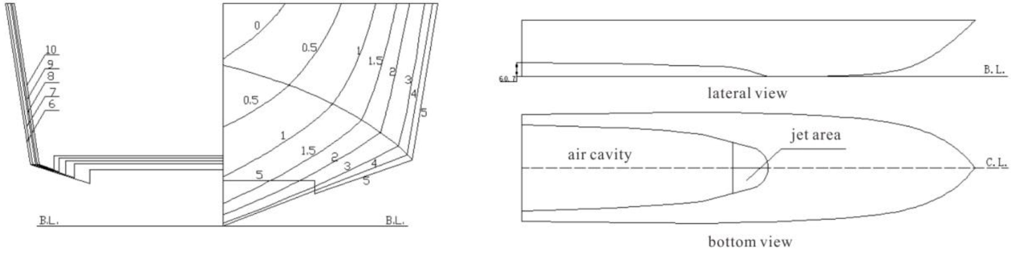
In China, Dong Wencai and Ou Yongpeng [11,12] from the Naval University of Engineering conducted experimental studies on air injection drag reduction for a B.H-type air-lubricated planing craft under calm water and wave conditions. As illustrated in Figure 2, the prototype vessel featured a non-stepped, deep-V planing hull designed with grooved regions extending from the midsection to the stern. The leading edge of the groove was arc-shaped when projected onto the horizontal plane, with the groove width gradually widening toward the stern. The groove bottom comprised either planar or folded planar surfaces, forming a developable surface. Their experiments examined the effects of speed, air injection rate, and waves on the hydrodynamic performance of the hull. Comparing two grooved hull designs with different groove depth transitions near the stepped region revealed that groove depth significantly affected navigation performance without air injection. The study concluded that the parameterized design of an air-lubricated planing craft is a promising and impactful avenue for future research in ALDR for planing vessels.

For low-speed, full-form ships, introducing localized air cavity structures generally has minimal impact on the navigation attitude of the vessel. Therefore, when implementing ALDR technology in these ships, the design and optimization of the air cavity structure can often be conducted independently. In contrast, adding air cavities in a planing craft significantly affects the flow field at the bottom of the hull. Additionally, since the air cavity substantially reduces the planing surface that provides dynamic lift, the craft’s running attitude is inevitably altered. Given the strong coupling effect between the air cavity and the hull, designing an air-lubricated planing craft from a hydrodynamic performance perspective requires not only the localized optimization of the air cavity structure but also a coordinated adjustment of the baseline planing hull’s lines based on air cavity parameters. Therefore, a holistic optimization approach that concurrently considers the design parameters of the air cavity and the planing hull is likely to enhance the overall optimal hydrodynamic performance of the air-lubricated planing craft.

With advancements in computational and CFD (computational fluid dynamics) technologies, integrating CFD-based numerical evaluation techniques with optimization theory and parameterized hull design methods has led to a new paradigm in hull design known as simulation-based design (SBD) [13]. This approach has been widely applied in the field of ship design. For air-lubricated planing hulls, SBD facilitates the exploration and optimization of the design space for vessel configurations through optimization techniques and geometric reconstruction methods, ultimately resulting in hydrodynamically optimal hull designs that operate under specific constraints. A key aspect of the SBD approach is hull parameterization.

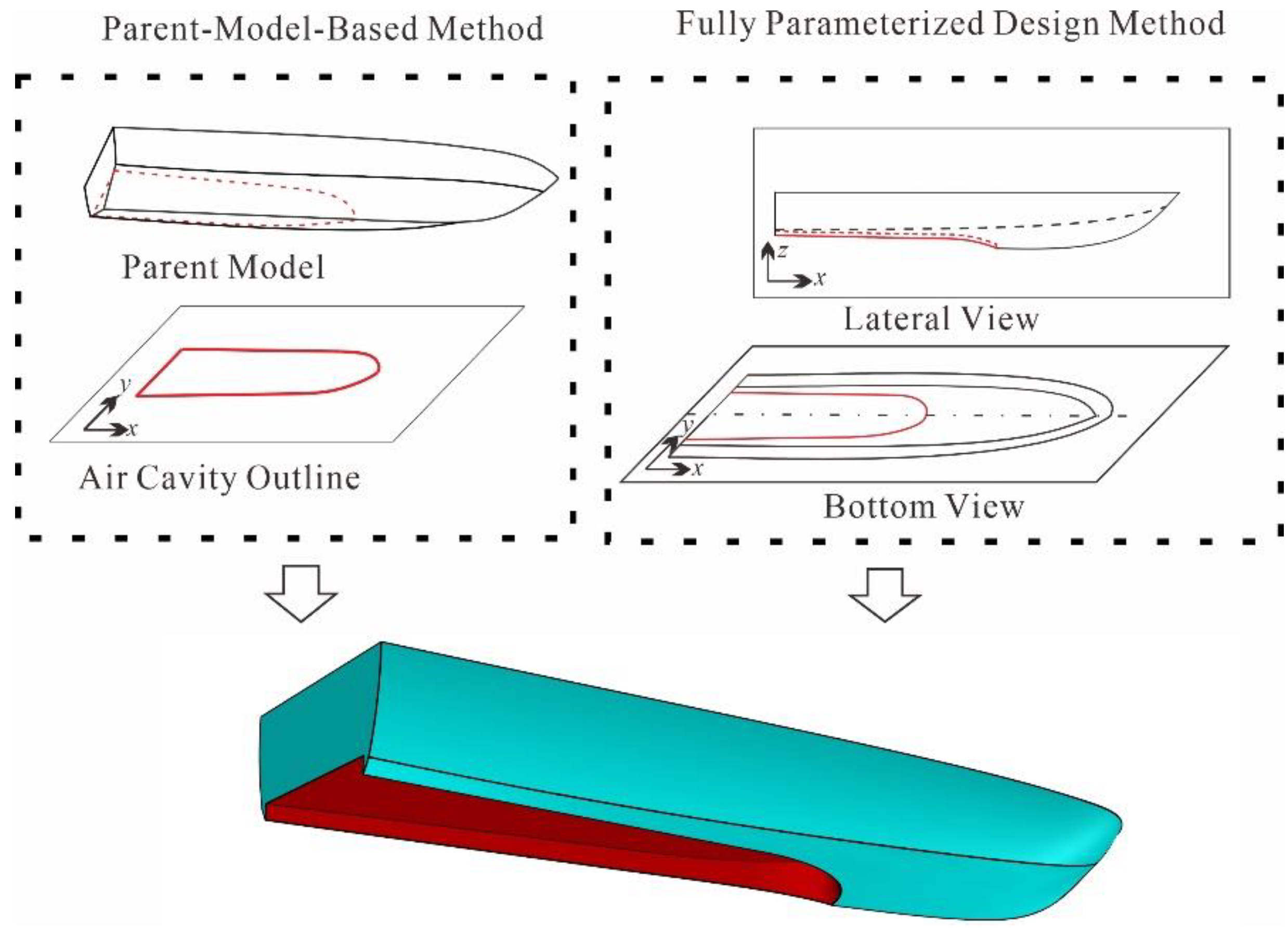
Rapid hull generation: In the SBD approach, many model samples must be computed. By developing an automated platform that integrates geometry generation, simulation, and optimization, the efficiency of the optimization process can be significantly enhanced [14]. As illustrated in Figure 3, the majority of air cavity planing hulls are derived through cutting and modification in the horizontal projection based on the parent model. When using this approach to generate a model for SBD, due to the extensive cutting of the running surface, a portion of the original design parameters becomes redundant. On the other hand, the spatial position of the air cavity edge line cannot be completely defined by the design parameters.

A fully parameterized modeling method entails sequentially defining and constructing the geometric model of the target vessel, from points to lines to surfaces, based on predetermined design parameter constraints. Notably, this method does not rely on an initial baseline hull and achieves a comprehensive definition of the vessel’s geometric features solely through design parameters. Consequently, a fully parameterized design of air-lubricated planing hulls offers several potential advantages.

Larger design space exploration: Traditional planing hulls, particularly those modified with air cavities, typically have design parameters confined to localized features associated with these cavities. In contrast, the fully parameterized design method allows for the direct definition of multiple geometric parameters of characteristic contour lines, including air cavity edge lines, across multiple sections. This enables the exploration and creation of a broader range of planing hull designs.

In the 1970s, Kuiper pioneered employing digital methods to represent hull surfaces [15]. From the 1990s onward, extensive research focused on parameterized hull modeling. Harries [16,17,18] proposed a parameterization method by developing F-spline curves and the corresponding design software CAESES. This software enables the deformation of hull lines based on specified parameters and has been extensively used to optimize hull hydrodynamic performance. Building on NURBS theory, Zhang et al. [19,20] identified longitudinal characteristic curves through feature parameters. They employed optimization methods to generate sectional station lines that were subsequently utilized to construct the hull surface.

Stemming from this representation, Lu [21] used NURBS functions to represent hull surfaces and explored critical issues in ship design. Kostas [22] employed T-splines in the Rhino modeling environment to develop hull surfaces with bulbous bows, achieving second-order continuity across the surface except at extraordinary points. Additionally, Mancuso [23] focused on a sailboat hull and establishing the keel and waterlines under parameter constraints while smoothing the hull surface using B-spline surfaces for parameterized modeling.

Zhou et al. [24] introduced a NURBS-based parameterization method for surface ships by using classifications of geometric feature parameters and designing characteristic curves to parameterize the hull surface. This method applied NURBS techniques to model hull curves and surfaces parametrically, enabling geometry-driven hull deformation and the development of the corresponding software.

Paérez-Arribas [25,26,27] adopted B-spline methods to parameterize various ship types, including surface ships, planing crafts, and small-waterplane-area twin hulls (SWATHs). Shahroz Khan [28] segmented yacht hulls into three regions and parameterized each section independently to produce a diverse array of hull designs. Ghassabzadeh [29] utilized three different geometric line types—parabolic, circular arcs, and NURBS curves—to design planing tunnel hulls.

Although substantial research has focused on the geometric parameterization of traditional hull types, studies focusing on fully parameterized modeling methods for air-lubricated planing crafts remain relatively scarce.

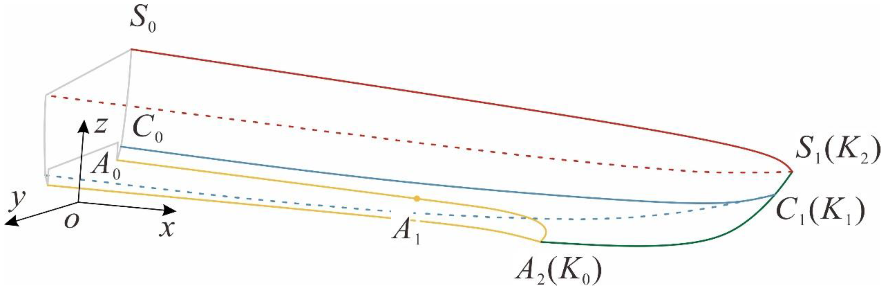
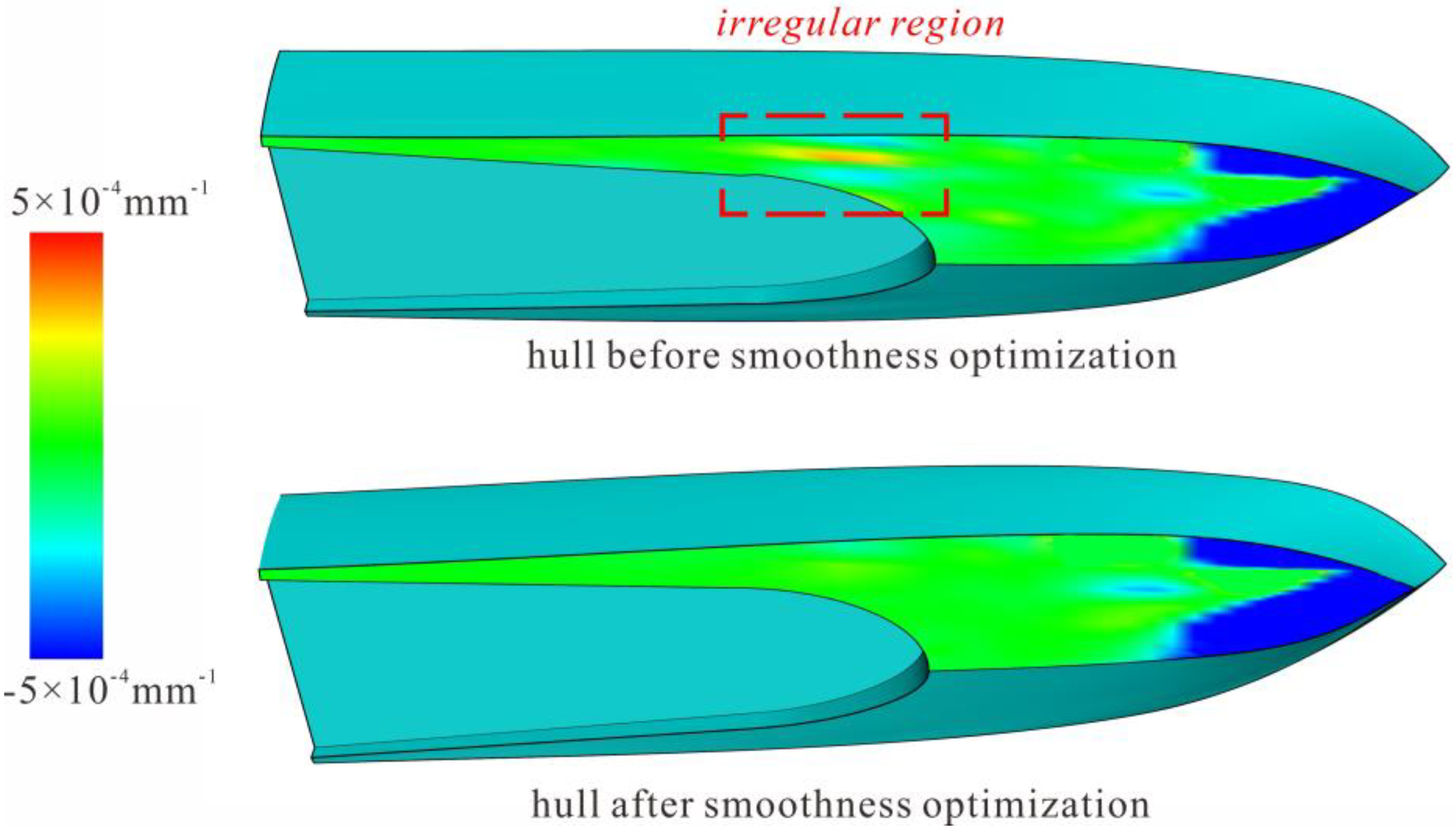
This study proposes a fully parameterized modeling method for air-lubricated planing crafts with air cavities. Unlike traditional techniques that involve adding grooves to traditional planing hulls to form an air-cavity hull, this approach defines a set of geometrically meaningful and mutually independent design parameters. These parameters are then utilized to construct the primary contour lines of the hull. Longitudinal functions associated with these design parameters generate sectional station lines for the major hull surfaces. Once the primary framework of the hull is established, an initial hull surface is fitted, followed by surface fairness optimization based on the principle of minimum strain energy.

As a demonstration, the proposed method is applied to the B.H-type air-lubricated planing hull [11,12] for modeling and deformation. The approach rapidly generates various smooth hull forms with distinct characteristics.

2. Modeling Methods

2.1. Fundamental Theory [30]

Non-uniform rational B-splines (NURBSs) are extensively utilized in ship geometric hull design due to their numerous advantages. They are considered the current industrial standard for representing, designing, and exchanging geometric models in computational applications. A NURBS curve of degree p can be defined as

$$C(u)={\displaystyle \frac{{\sum }_{i=0}^n{N}_{i,p}(u){\omega }_i{\mathit{P}}_i}{{\sum }_{i=0}^n{N}_{i,p}(u){\omega }_i}},0\le u\le 1$$

(1)

where P_i represents the control points, ω_i is the weight factor, and $N_{i,p}(u)$ is the p-degree B-spline basis function defined over a non-periodic knot vector U. The basis function $N_{i,p}(u)$ is calculated using the Cox–de Boor recursion formula.

A NURBS curve is an extension of a B-spline curve with the addition of weight functions. A B-spline curve is a special case of a NURBS curve when all weight coefficients are equal to 1. The normalized p-degree B-spline curve can be defined as

$$C(u)=\sum _{i=0}^n{N}_{i,p}(u){\mathit{P}}_i$$

(2)

A B-spline surface of degree p in the u-direction and degree q in the v-direction is a bivariate; the piecewise-defined rational function is expressed as

$$S(u)=\sum _{i=0}^n\sum _{j=0}^m{N}_{i,p}(u)N_{j,q}(v){\mathit{P}}_{i,j},0\le u,v\le 1$$

(3)

This paper collectively refers to Bézier curves as B-spline curves for simplicity in description. When the basic functions of a B-spline curve with p-degree and p + 1 control points are defined over the clamped knot vector ${\mathit{U}}_B=\{\underset{p+1}{\underbrace{0,0\dots ,0}},\underset{p+1}{\underbrace{1,1\dots 1}}\}$, the B-spline curve becomes equivalent to a Bézier curve:

$$C(u)=\sum _{i=0}^p{B}_{i,p}(u){\mathit{P}}_i$$

(4)

The corresponding first-order derivative equation is expressed as

$$C^{\prime }(u)=\sum _{i=0}^p{B}_{i,p}^{\prime }(u){\mathit{P}}_i$$

(5)

In this equation, $B_{i,p}^{\prime }(u)$ is obtained by taking the derivative of the corresponding basis function $B_{i,p}(u)$ with respect to u. The second- and third-degree Bézier curve basis functions and their first-order derivatives used in this study are shown in

Table 1. Second- and third-degree Bézier curve basis functions and their first-order derivatives.

i	${\mathit{B}}_{\mathit{i}}^3(\mathit{u})$	${{\mathit{B}}^{\mathit{\prime }}}_{\mathit{i}}^3(\mathit{u})$	${\mathit{B}}_{\mathit{i}}^2(\mathit{u})$	${{\mathit{B}}^{\mathit{\prime }}}_{\mathit{i}}^2(\mathit{u})$
0	$(1-u{)}^3$	$-3(1-u{)}^2$	$(1-u{)}^2$	$-2(1-u)$
1	$3u(1-u{)}^2$	$3(1-u{)}^2-6u(1-u)$	$2u(1-u)$	$2-4u$
2	$3u^2(1-u)$	$6u(1-u)-3u^2$	$u^2$	$2u$
3	$u^3$	$3u^2$

.

2.2. Types of Principal Hull Contour Lines

The hull of an air-lubricated planing craft featuring air cavities consists of several principal contour lines, including the sheer line S₀S₁, the chine line C₀C₁, the air cavity edge line A₀A₁A₂, and the keel line K₀K₁K₂, as illustrated in Figure 4. These lines define the boundaries of the primary hull surfaces and constitute the main framework of the hull. To achieve fully parameterized modeling of the air-lubricated planing hulls, selecting a suitable curve to represent the principal hull contour lines accurately is essential.

In the hull coordinate system used during the design phase, most characteristic contour lines are spatial curves that can be jointly defined by their projections onto two orthogonal planes. For the planar projection curves of these principal contour lines, it is important to choose appropriate curve types and their geometric constraints based on the design requirements, as outlined in

Table 2. Principal hull contour line projections and geometric constraints.

Contour Lines	Projection Plane	Curve Types	Geometric Constraint Conditions
A0A1	xoy	linear segment
A0A1	xoz	linear segment
A1A2	xoy	Cubic Bézier Curve	C1-Continuity with A0A1 at A1
A1A2	xoz	Cubic Bézier Curve	C1-Continuity with A0A1 at A1
K0K1	xoz	Cubic Bézier Curve	K0 = A2
K1K2	xoz	Quadratic Bézier Curve	C1-Continuity with K0K1 at K1
C0C1	xoy	Cubic Bézier Curve	C1 = K1
C0C1	xoz	Cubic Bézier Curve	x(C0) = x(A0)
S0S1	xoy	Cubic Bézier Curve	S1 = K2
S0S1	xoz	Linear Segment	x(S0) = x(A0)

. This selection process determines the independent design parameters needed for the characteristic contour lines and establishes the basis for selecting the design parameter set.

2.3. Design Parameters

The selection of appropriate design parameters is crucial for optimizing hull design methods. The approach to parameter selection must involve the careful evaluation of specific design objectives and application scenarios. In this paper, the design parameters are categorized into two types based on the design steps.

The first type of design parameters, shown in

Table 3. The first type of design parameters.

Location	Symbol	Parameter Description	Value
Air cavity	LA1	Straight segment longitudinal length of the air cavity.	1311 mm
	LA2	Overall longitudinal length of the air cavity.	1791 mm
	BA0	Stern-end width of the air cavity.	273.6 mm
	BA1	Curved segment width of the air cavity.	212.5 mm
	HA0	Stern-end height of the air cavity edge line.	91.1 mm
	HA1	Height of the air cavity edge line at the transition point.	65 mm
	HA2	Height of the step tip point.	0 mm
	λA1	Shape factor of the horizontal projection of the air cavity edge line’s curved segment.	0.63
	λA2	Shape factor of the horizontal projection of the air cavity edge line’s curved segment.	0.12
	ωA1	Shape factor of the side projection of the air cavity edge line’s curved segment.	0.6
	ωA2	Shape factor of the side projection of the air cavity edge line’s curved segment.	0.14
Chine	Lc1	Longitudinal length of the chine.	2764 mm
	Bcm	Maximum width of the chine.	622 mm
	BC0	Stern-end width of the chine.	300 mm
	Lcm	Longitudinal coordinate of the maximum width point of the chine.	1184 mm
	βc	Tangent angle at the end of the chine’s horizontal projection.	39.7°
	γA0	Stern-end transverse deadrise angle.	38°
	γA1	Transverse deadrise angle at A1.	37.2°
	γA2	Transverse deadrise angle at A2.	35°
	HC1	Bow-end height of the chine.	260.7 mm
Sheer	Ls1	Longitudinal length of the sheer.	2867 mm
	Hs1	Bow-end height of the sheer.	360 mm
	Hs0	Stern-end height of the sheer.	360 mm
	Lsm	Longitudinal coordinate of the maximum width point of the sheer.	1316 mm
	Bsm	Maximum width of the sheer.	702 mm
	BS0	Stern-end width of the sheer.	335 mm
	βS	Tangent angle at the end of the sheer’s horizontal projection.	51.1°
Keel	ωK1	Shape factor of the keel line curve’s lifting segment.	0.6
	ωK2	Shape factor of the keel line curve’s lifting segment.	0.27
	βk	Tangent angle at the K2 of the keel’s side projection.	44°

, consists of the primary dimensional parameters. The designer defines the parameters that possess intuitive geometric significance, such as hull length, hull width, and key point coordinates. The first type of design parameters directly and independently influences the characteristic contour lines of the hull, facilitating the control and modification of the hull’s overall primary dimensions and features.

The second type of design parameters consists of surface shape control parameters, a portion of which are expressed in the form of longitudinal functions. These parameters are independent of the first type of design parameters and are used to define the geometric characteristics of the hull’s sectional station lines based on the established hull contour lines. By defining the second type of design parameters, modifications to the shapes of the sectional station lines can be achieved, enabling further adjustments to the surface shape characteristics of the hull. The values of the second type of design parameters for the target hull form are presented in

Table 4. The second type of design parameters.

Location	Symbol	Parameter Description	Mathematical Representation
Air cavity	t	Depth distribution of the air cavity along the x-direction.	$t(x)=(H_{A0}-h_a(x))+45$
Side surface	ks1	Shape factor of the extreme position distribution for side surface station lines.	ks1 = 0.5
	ks2	Shape factor of the side surface station line curvature.	$k_{s2}(x)=0.04+0.02x/L{s}_1$
Planing surface	kp1	Shape factor of the extreme position distribution for planing surface station lines.	kp1 = 0.5
	kp2	Shape factor of the planing surface station line curvature.	$k_{p2}(x)=\left\{\begin{array}{l}-0.04(x-1500)/(L_{s1}-1500),x>1500\\ 0\hspace{1em}\hspace{1em}\hspace{1em}\hspace{1em}\hspace{1em}\hspace{1em}\hspace{1em}\hspace{1em}\hspace{1em}\hspace{1em} ,x\le 1500\end{array}\right.$

.

2.4. Principal Hull Contour Lines

2.4.1. Derivation of Control Points for Planar Projection Lines

In this study, B-spline curves are primarily employed to represent the planar projections of the primary hull contour lines. The design parameters determine the coordinates of the two endpoints of these curves. In contrast, the coordinates of the intermediate control points are typically treated as unknowns, defined by the first type of design parameters and various geometric continuity conditions. By utilizing Equations (4) and (5), corresponding constraint equations can be established, facilitating the construction of a system of equations for the curves on each projection plane. Once the values of the first type of design parameters are substituted, the unknown control point coordinates of the projection curves can be resolved.

The specific solving process is demonstrated using the cavity edge line of the cavity as an example. As illustrated in Figure 5, the cavity edge line consists of two segments. A₀A₁ is a linear segment, while A₁A₂ is a spatial curve segment, solved separately in the horizontal and side-view projection planes.

In the horizontal projection plane, the projection curve is defined as a cubic Bézier curve with four control points.

$${\mathit{S}}_{A-xy}(u)=B_0^3(u){\mathit{A}}_1+B_1^3(u){\mathit{C}}_1+B_2^3(u){\mathit{C}}_2+B_3^3(u){\mathit{A}}_2$$

(6)

The curve ${\mathit{S}}_{A-xy}(u)$ satisfies the following conditions: The curve passes through point A_m. At P_k2, the slope of the curve is equal to the slope of the chord. At A₁, the curve satisfies continuity with the straight line A₀A₁, and the slope ${\mathit{\eta }}_1$ at A₁ is derived directly from the slope of the straight line A₀A₁.

Based on these conditions, a system of linear equations can be established:

$$\begin{gathered} \left[\begin{array}{cccc}{B}_1^3\left(u_m\right)& 0& B_2^3\left(u_m\right)& 0\\ 0& B_1^3\left(u_m\right)& 0& B_2^3\left(u_m\right)\\ {\mathit{\eta }}_1{B^{\prime }}_1^3& -{B^{\prime }}_1^3\left(u_m\right)& {\mathit{\eta }}_1{B^{\prime }}_2^3\left(u_m\right)& -{B^{\prime }}_2^3\left(u_m\right)\\ {\mathit{\eta }}_m& -1& 0& 0\end{array}\right]\left[\begin{array}{c}{X}_{C1}\\ Y_{C1}\\ X_{C2}\\ Y_{C2}\end{array}\right]= \\ \left[\begin{array}{c}{X}_{Am}-B_0^3\left(u_m\right)L_{A1}-B_3^3\left(u_m\right)L_{A2}\\ Y_{Am}-B_0^3\left(u_m\right)B_{A1}-B_3^3\left(u_m\right)0\\ {B^{\prime }}_0^3\left(u_m\right)B_{A1}+{B^{\prime }}_3^3\left(u_m\right)0-{\mathit{\eta }}_1{B^{\prime }}_0^3\left(u_m\right)X_{A1}-{\mathit{\eta }}_1{B^{\prime }}_3^3\left(u_m\right)X_{A2}\\ {\mathit{\eta }}_m{L}_{A1}-B_{A1}\end{array}\right] \end{gathered}$$

(7)

In this equation, ${\mathit{\eta }}_1$ represents the tangential slope at A₁ with respect to the straight line A₀A₁; ${\mathit{\eta }}_m$ represents the slope of the chord A₁A₂; X_Am denotes the x-coordinate value of point A_m; u_m represents the curve parameter corresponding to point A_m, which can be calculated using the chord length parameterization method:

$$u_m={\displaystyle \frac{\left|A_m-A_1\right|}{\left|A_2-A_m\right|+\left|A_m-A_1\right|}}$$

(8)

By solving Equation (7), the coordinates of the unknown control points C₁ and C₂ for the curve can be obtained. In the side-view projection plane, the contour curve’s projection is defined as a cubic Bézier curve with four control points:

$${\mathit{S}}_{A-xz}(u)=B_0^3(u){\mathit{A}}_1+B_1^3(u){\mathit{C}}_3+B_2^3(u){\mathit{C}}_4+B_3^3(u){\mathit{A}}_2$$

(9)

The curve design parameters include H_A1, L_A1, and L_A2. Similar to the method used to solve for the control points C₁ and C₂ in the xoy-plane, a system of equations is established and solved to determine the coordinates of the control points C₃ and C₄.

2.4.2. Generating Spatial Curves from Planar Curves:

Along the longitudinal range of A₀A₁, n coordinate values are sampled equally. First, the value of the parameter u_i corresponding to Equation (9) is calculated. The parameter equation for the x-component of the lateral projection curve is as follows:

$$x_i={\left(1-u_i\right)}^3\cdot x_{A1}+3u_i{(1-u_i)}^2\cdot x_{C3}+3{u_i}^2(1-u_i)\cdot x_{C4}+{u_i}^3\cdot x_{A2}$$

(10)

Equation (10) can be solved numerically using Newton’s iteration method. After obtaining the value of the parameter u_i, the z-coordinate of the point can be calculated as

$$z_i={\left(1-u_i\right)}^3\cdot z_{A1}+3u_i{(1-u_i)}^2\cdot z_{C3}+3{u_i}^2(1-u_i)\cdot z_{C4}+{u_i}^3\cdot z_{A2}$$

(11)

Similarly, the corresponding coordinate y_i can be obtained, resulting in a set of discrete points, Q(x_i,y_i,z_i), of A₀A₁. By applying the least-squares method, the control point P_i of the spatial curve can been created.

$$S_A(u)={\displaystyle \sum _{i=0}^{n+2}{N}_{i,3}(u)P_i}$$

(12)

2.5. Sectional Station Lines

The primary characteristic contour lines of the hull serve as the boundaries of the hull surface, and sufficiently dense sectional station lines can act as the framework to define the shape of the hull surface. Based on the main surfaces of the hull, the sectional station lines can be categorized into three groups: air cavity surface sectional station lines, planing surface sectional station lines, and side surface sectional station lines. The discrete points corresponding to the contour lines are used as endpoints of the sectional station lines, and the second type of design parameters is utilized to define each sectional station line fully.

2.5.1. Design of Air Cavity Sectional Station Lines

The top and side surfaces of the air cavity are developable folded surfaces. In this study, the cross-sectional station lines of the air cavity are designed as right-angled polyline segments. For the i-th air cavity sectional station line, the required design parameter is the depth t_i, which can be calculated as a function of the longitudinal coordinate x of the i-th section using t(x):

$$t\left(x\right)=k_1\times \left(H_{A0}-h_a\left(x\right)\right)+k_2\times x+t_{a0}$$

(13)

where ha(x) is the z-coordinate value of the discrete point A_i on the air cavity edge line at x; t_a0 is the air cavity depth at point A₀.

Experimental results from [6] indicate that there exists an optimal longitudinal trim angle for planing crafts that maximize the steady-state air-layer area. Thus, the parameters k₁ and k₂ are introduced to modify the depth distribution of the air cavity’s inner wall and its overall slope.

Figure 6 shows the influence of the coefficients k₁ and k₂ on the air cavity depth distribution. k₁ controls the relative depth distribution of the air cavity. When k₁ = 0, the inner wall characteristic curve B₀B₁ is parallel to the edge line. As k₁ approaches 1, the curve B₀B₁ becomes straighter. k₂ controls the overall inclination of the top plate curve.

By adjusting the values of k₁ and k₂, it is possible to effectively define the longitudinal distribution of the air cavity cross-sectional area, the depth at the bow step, and the slope of the straight section.

In [12], two air cavity depth distribution schemes were studied for their effects on hydrodynamic performance: The first one corresponds to the depth design parameters of k₁ = 1 and k₂ = 0. The second one corresponds to the design parameters in this study, k₁ = 0 and k₂ = 0.

2.5.2. Side and Planing Surface Sectional Station Lines

As illustrates in Figure 7, the side sectional station lines are represented using a quadratic B-spline curve with three control points. For any given section j, the endpoints S_j and C_j are determined by discretizing and solving the contour lines. The intermediate control point D_j is defined to control the concave or convex shape of the side sectional station line. The construction method for the planing surface sectional station lines is similar.

The coordinates of the control point D_j are expressed relative to the endpoints S_j and C_j:.

$${\mathit{D}}_j={\mathit{S}}_j+k_{s1}{\overrightarrow{{\mathit{S}}_j\mathit{C}}}_j+k_{s2}\mathit{n}$$

(14)

where n is a vector perpendicular to the chord line S_jC_j with equal length on both sides.

2.6. Skinning

Upon completing the design of the sectional station lines, the primary surfaces of the hull, such as the side surface, planing surface, and inner wall surface of the air cavity, are generated based on these sectional station lines. For each hull surface, once the sectional station lines are established, discrete surface points can be generated from the equations of the sectional station lines. A (p,q)-degree B-spline tensor product surface is then created to interpolate these discrete points; they are expressed as

$${\mathit{Q}}_{k,l}=\mathit{F}\left(u_k,v_l\right)=\sum _{i=0}^n\sum _{j=0}^m{N}_{i,p}\left(u_k\right)N_{j,q}\left(v_l\right){\mathit{P}}_{i,j}=\sum _{i=0}^n{N}_{i,p}\left(u_k\right)\left(\sum _{j=0}^m{N}_{j,q}\left(v_l\right){\mathit{P}}_{i,j}\right)$$

(15)

Let ${\mathit{R}}_{i,l}={\sum }_{j=0}^m{N}_{j,q}\left(v_l\right){\mathit{P}}_{i,j}$ then:

$${\mathit{Q}}_{k,l}=\sum _{i=0}^n{N}_{i,p}\left(u_k\right){\mathit{R}}_{i,l}$$

(16)

At this point, the surface interpolation problem is reduced to one of curve interpolation. By applying curve interpolation n + 1 times, the control point ${\mathit{R}}_{i,l}$ for the curves can be solved. Similarly, by performing m + 1 interpolations on ${\mathit{R}}_{i,l}$, the control point ${\mathit{P}}_{i,j}$ of the surface can be obtained. Substituting ${\mathit{P}}_{i,j}$ into Equation (15) forms the interpolating surface.

2.7. Air Injection Holes

Air injection holes are generally distributed on the upper surface inside the air cavity, which is convenient for connection with the air injection device inside the hull. The shape and distribution form of the air holes can be designed in different ways according to different engineering requirements. Since the air flow rate is a more critical factor for the stability of the air layer, the air injection holes should be designed to have a large enough total area to ensure the air flow rate. Based on the experience of the air cavity planing hull experiment and CFD research, it is recommended to distribute them at the front part of the air cavity.

2.8. Design Process

The parametric generation process of the air cavity planing hull model is illustrated in Figure 8.

3. Smoothness Optimization

3.1. Smoothness Criteria

The smoothness of curves and surfaces in ship hull design is not only essential for the esthetic appearance of the vessel, but it also has a significant impact on manufacturing processes and hydrodynamic performance. Therefore, optimizing the smoothness of the hull during parametric design is a necessary and practically meaningful task.

Designing smooth curves and surfaces engages multiple disciplines, and subjective perceptions of smoothness can vary from person to person. As a result, there is no universally accepted standard for smoothness within academia. However, in ship surface design, the following criteria are widely acknowledged as fundamental requirements for smoothness [31]:

(1)

Continuity of Curves and Surfaces: curves and surfaces must maintain a certain degree of continuity;

(2)

Absence of Redundant Singularities and Inflection Points: no unnecessary singularities or inflection points should exist;

(3)

Uniform Curvature Variation: the curvature of curves and surfaces should change uniformly;

(4)

Minimized Strain Energy: the strain energy of the curves and surfaces should be as small as possible.

According to the modeling approach outlined in Section 2, the hull designed using the fully parameterized method is presented in Figure 9. Near the forward region of the slotted area at the bottom of the hull, noticeable non-smoothness irregularities can be observed along the edges, accompanied by an uneven surface curvature. While the cubic B-spline surfaces and curves employed in the modeling process maintain continuous second-order derivatives, local distortions occur due to an inappropriate selection of design parameters, leading to excessive curvature variations in the local curves and surfaces. To enhance surface smoothness, the original design parameters are optimized to minimize strain energy.

3.2. Objective Function and Selection of Optimization Parameters Based on the Minimum Strain Energy Principle

The goal of smoothness optimization is to coordinate local design variables to ensure that the planing surface and edge lines are as smooth as possible. Based on the curvature, the surface and curve strain energy are defined, as shown in Equations (17) and (18) [32].

$$E\mathrm{c}={\displaystyle \int {\kappa }^2}du$$

(17)

$$E\mathrm{s}={\displaystyle \iint \left({\kappa }_1^2+{\kappa }_2^2\right)}dudv$$

(18)

where κ represents the curvature of the curve, and κ₁ and κ₂ are the principal curvatures of the surface.

Taking the minimization of the planing surface strain energy and the minimization of the air cavity edge line strain energy as the optimization objectives, all design parameters of the hull are listed in Table 2. However, treating all design parameters as optimization variables is inappropriate. For instance, parameters such as hull length and hull width must be defined by the designer and cannot be altered. Instead, flexible parameters that locally influence the non-smooth regions can be selected as the optimization variables. In this study, the optimization parameters $X=({\lambda }_{A1},{\lambda }_{A2})$ are selected from the air cavity edge line.

According to the content in Section 2, a spatial curve of A₁A₂ is established with the parameters in Table 3, and the equation of the A₁A₂ curve is S_A(u), as shown in Equation (12). The curvature formula at an arbitrary point S_A(u_i) is

$$\kappa (u_i)={\displaystyle \frac{‖{\dot{S}}_A(u_i)\times {\ddot{S}}_A(u_i)‖}{{‖{\dot{S}}_A(u_i)‖}^3}}$$

(19)

where ${\dot{S}}_A(u_i)$ and ${\ddot{S}}_A(u_i)$ are, respectively, the first-order and second-order derivatives of $S_A(u)$ with respect to u at u_i. The strain energy of the curve at this time is calculated by substituting it into Equation (17) using the numerical integration method:

$$E\mathrm{c}={\displaystyle \sum _{i=1}^n\left[({\kappa }^2(u_{i-1})+{\kappa }^2(u_i))\cdot (u_i-u_{i-1})\right]}$$

(20)

Similarly, the planing surface is discretized in the u and v directions. As shown in Figure 10, Es can be calculated using numerical methods:

$$E\mathrm{s}={\displaystyle \sum _{j=1}^m{\displaystyle \sum _{i=1}^n\left[({{\kappa }_1}^2(u_i,v_j)+{{\kappa }_2}^2(u_i,v_j))\cdot (u_i-u_{i-1})(v_i-v_{i-1})\right]}}$$

(21)

This process enables the calculation of the curve strain energy Ec(X) and the surface strain energy Es(X) under the given parameter $X=({\lambda }_{A1},{\lambda }_{A2})$. The objective function is then defined as

$$\left\{\begin{array}{c}{f}_1=Es(X)\\ f_2=Ec(X)\end{array}\right.$$

(22)

The upper and lower bounds of the optimization parameters are constrained based on the geometric modeling feasibility, resulting in the following constraint conditions:

$$\left\{\begin{array}{c}0<{\lambda }_{A1}<1\\ 0<{\lambda }_{A2}<1\end{array}\right.$$

(23)

At this point, the hull smoothness optimization problem is transformed into a multi-objective optimization problem, with Equation (22) as the objective function and Equation (23) as the constraint condition.

3.3. Optimization Algorithm

The NSGA-II algorithm [33], proposed by Deb et al., is a multi-objective optimization algorithm based on Pareto optimality. It addresses the inefficiencies and poor convergence issues of the original NSGA and has been widely applied in fields such as machine learning and combinatorial optimization. The steps of the algorithm are as follows:

• Initialization: Randomly generate an initial population, P₀, of size N. Perform non-dominated sorting, and use the three basic genetic operations—selection, crossover, and mutation—to generate the first-generation offspring population Q₀ of size N;
• Population Combination and Sorting: From the second generation onward, combine the parent population P_n and the offspring population Q_n into a combined population, R_n, of size 2N. Perform fast non-dominated sorting to obtain the non-dominated fronts F₁,F₂, …;
• Crowding Distance and Selection: Calculate the crowding distance for each individual in the non-dominated fronts. Based on the non-dominated ranking and crowding distance, select N individuals to form the new parent population P_n+1;
• Offspring Generation: perform the basic genetic operations (selection, crossover, and mutation) to generate the new offspring population Q_n+1, thereby completing one evolutionary step;
• Termination: Repeat Steps 2–4 until the maximum number of generations is reached. At this point, the algorithm outputs the Pareto-optimal solutions for the optimization problem.

Parameter Settings:

Population size: 100

Crossover probability: 0.9

Mutation probability: 0.1

Maximum number of generations: 200

The Pareto-optimal solutions are obtained by iterating the optimization problem defined in Section 3.2, as shown in Figure 11.

3.4. Multi-Objective Decision-Making Method

Since achieving optimal solutions for all objective functions simultaneously is impossible, the Pareto-optimal solution set of the objective functions must be analyzed comprehensively based on actual requirements. A decision must be made to select the best solution that is closest to the optimal values of the objectives. The specific multi-objective decision-making method adopted in this study is as follows.

Step 1: Determine Subjective Weight Coefficients Using Expert Scoring

The expert scoring method is used to calculate the subjective weight coefficients. The experts include professors specializing in naval architecture from various universities, engineers from ship design institutes, and designers from ship production units. Based on their experiences in their respective fields, the experts evaluate the importance of smoothness in local curves and surfaces during the modeling process. The importance is scored on a scale from 1 to 5, with the results shown in

Table 5. The experts’ scoring result.

Target	Expert 1	Expert 2	Expert 3	Expert 4	Expert 5	Expert 6	Expert 7	Expert 8	Expert 9	Expert 10
Surface	5	4	5	3	5	4	4	4	5	5
Edge	3	3	5	4	2	3	2	2	3	2

.

Step 2: Calculate Objective Weights

Let the normalized Pareto solution set from Section 3.3 be S = (s_ij)_14×2. The objective weight ω_n for the two indicators is calculated using the COWA operator [34].

$${\omega }_n={\displaystyle \frac{{\omega }_n^{*}}{\sum {\omega }_n^{*}}}$$

(24)

Step 3: Combine Subjective and Objective Weights

Using the linear coefficients λ₁ and λ₂, the objective and subjective weights are combined to minimize the deviation between the resulting comprehensive weight and the original objective and subjective weights. The weights are applied to the elements of S = (s_ij)_14×2 to produce K = (k_ij)_14×2.:

Step 4: Select the Optimal Solution

Based on K, the proximity index of each individual in the Pareto solution set to the optimal level is calculated. The individual with the maximum proximity index is selected as the optimal solution. The optimal solution is calculated to be ${\lambda }_{A1}=0.7548 \mathrm{a}\mathrm{n}\mathrm{d}{ \lambda }_{A2}=0.0657$, where $Es\left(X\right)=37.229 \mathrm{a}\mathrm{n}\mathrm{d} Ec(X)=0.10301$. The hull shape optimized for smoothness is shown in Figure 12.

4. Modeling Example

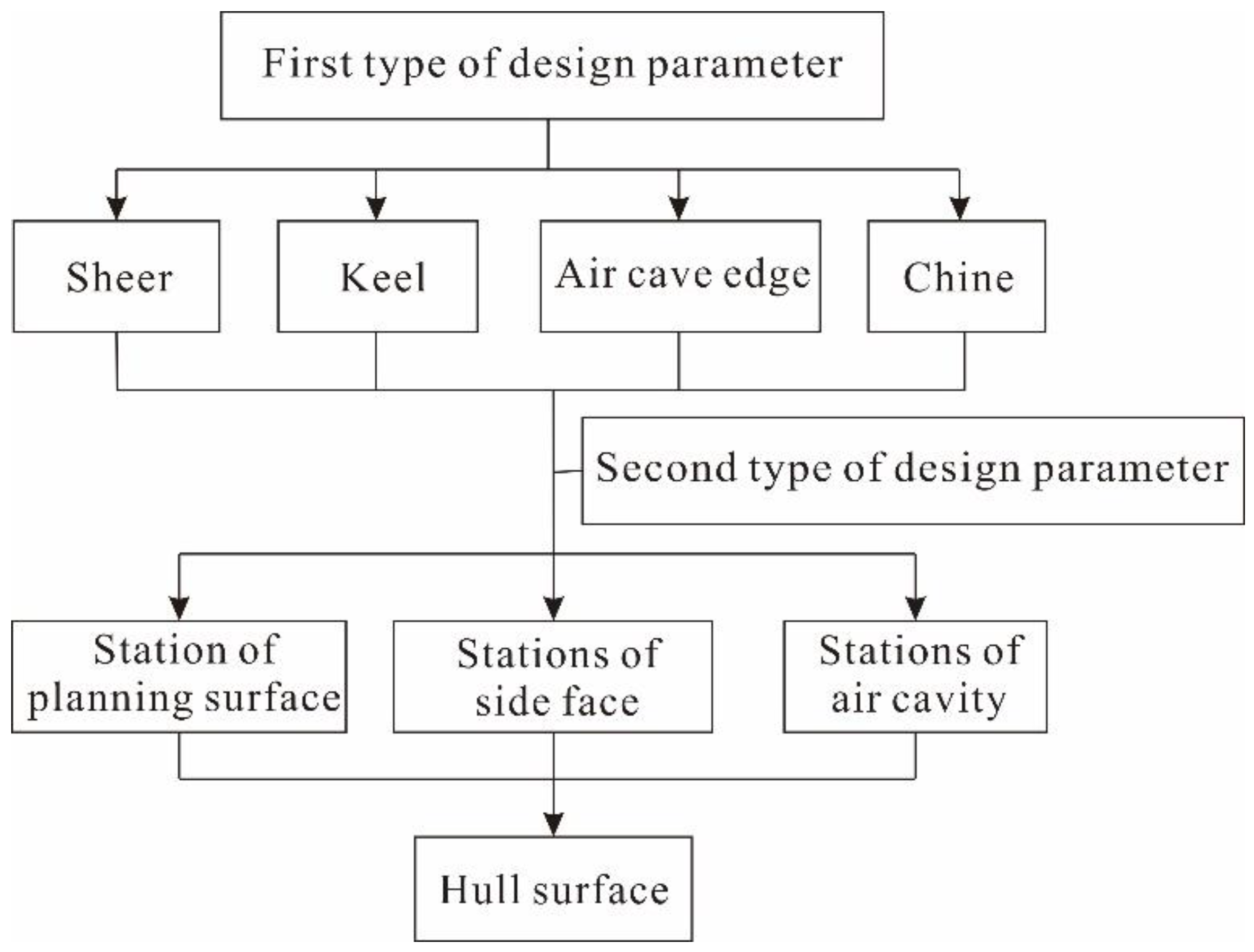
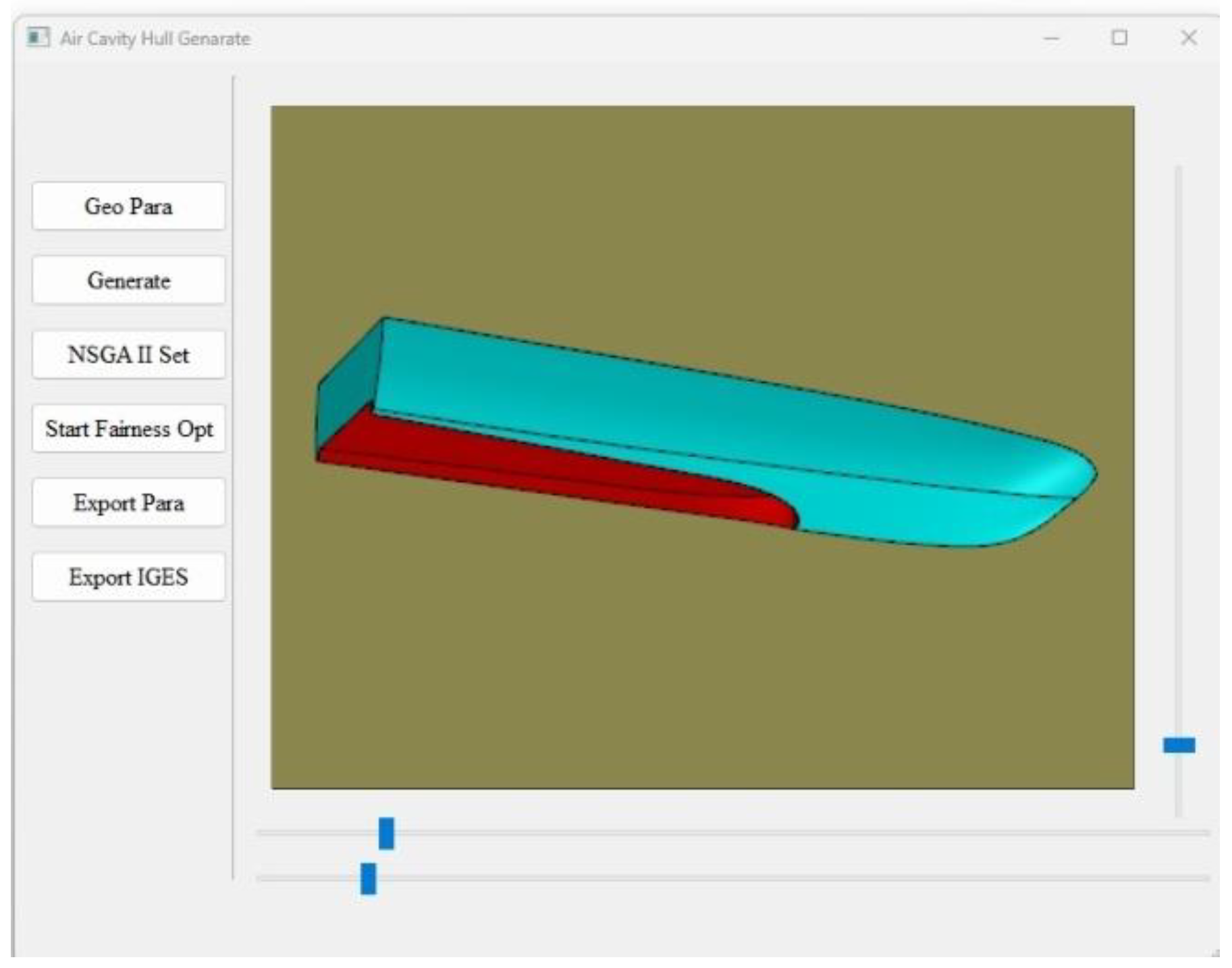
As illustrated in Figure 13, a modeling program for air-lubricated planing hull has been developed based on the methods described in this paper. The user interface (UI) is built on Qt, a cross-platform development framework, while the core modeling and smoothness optimization functions are implemented in backend C++ files. The program comprises two key functionalities: fully parameterized modeling and local parameter optimization.

Following the content in Section 2, users can define the first and second types of parameters to generate the initial hull form through the point-line-surface process sequentially. According to the content in Section 3, users can define the relevant parameter settings for the NSGA-II algorithm to achieve smoothness optimization for the hull.

The primary application of the parametric modeling of the air-lubricated planing hull lies in providing effective geometric models for the overall hull parameter optimization design, as illustrated in Figure 14. By adjusting specific geometric parameters, hull forms with different characteristics can be generated, validating the effectiveness of the proposed modeling method.

Model 1: this model closely resembles the original hull form, with its parameter values listed in Table 2 and Table 3.

Model 2: This design adopts a style similar to a flat-bottomed high-speed boat. The modified parameters are outlined in

Table 6. Modified parameters of Model 2.

HA0	HA1	γA0	γA1	γA2
20 mm	18 mm	17°	21°	23°	$15$

, while the other parameters remain the same as those in Model 1. The height of the air cavity edge line has been reduced, and the aft transverse deadrise angle is decreased, resulting in a lower side angle. The mid-to-aft section of the hull becomes lower and smoother, providing relatively more internal arrangement space. Additionally, the air cavity depth is smaller and uniformly distributed, which is expected to reduce the form drag resistance in non-air-lubricated conditions. Model 1 is modified into Model 2 with the parent-model-based method, as illustrated in Figure 14. Since there are only the parameters of the horizontal projection curve of the cavity edge, the parameters in the height direction such as H_A0, H_A1, and γ_A cannot be defined; that is, the parameters related to the side view of the air groove cannot be defined. On the other hand, since a considerable part of the planing surface will be cut off, many design parameters set for the original surface fail to be fully utilized. These redundant parameters not only augment the intricacy of the design process, but they also have the potential to impose unwarranted encumbrances on the optimization endeavors of the hydrodynamic performance.

Model 3: This model incorporates a longer air cavity design, with the significant modifications specified in

Table 7. Modified parameters of Model 3.

LA2	LA1	ωK1	ωK2	γA0	γA1	γA2	$\mathit{t}(\mathit{x})$
2159.2 mm	1573.2 mm	0.57	0.31°	17°	28°	36°	$t(x)=1\times (H_{A0}-h_a(x))+55$

, while $t(x)$ and other parameters remain the same as those in Model 1. Compared to Models 1 and 2, the step location is moved forward, and the keel design in the forward section is steeper. This configuration is expected to create a larger stable air-layer area.

5. Conclusions

This study proposes a fully parameterized modeling approach for an air-lubricated planing craft with air cavities. Using the B.H-type air-lubricated planing craft as the research object, the modeling process categorizes design parameters into two types:

• First-Type Parameters: These parameters are used to construct linear equation systems to establish planar projection curves of contour lines, such as the air cavitiy edge line. After solving these equations, the planar projection curves of the primary contour lines are obtained. These are then fitted to form spatial curves of the primary contour lines, which act as the main framework;
• Second-Type Parameters: This category defines a series of longitudinal functions that further delineate the principal geometric characteristics of sectional station lines for various surfaces. Once the hull framework of the sectional and contour lines is established, the complete hull surface is constructed using surface interpolation methods based on NURBS theory.

Certain parameters are redefined as optimization variables to tackle the local non-smoothness issues that arise from directly defining design parameters. Using the minimum strain energy principle, the multi-objective NSGA-II method is employed to minimize the local curve and surface strain energy, resulting in a Pareto solution set. This Pareto set selects the optimal solution, producing a smooth hull surface.

A program was developed based on the proposed method, generating multiple air-lubricated planing craft models. The generated hulls exhibit surface continuity and smooth appearance.

Here are conclusions and perspectives:

• Hull Design Framework: Based on NURBS and B-spline theories, a hull form can be designed sequentially from points to lines to surfaces by combining design parameters and constraints. This process enables the preliminary generation of models for air-lubricated planing crafts.
• Challenges in Direct Parameter Definition: when the designer directly defined all design parameters, particularly in the complex forward region of the air cavity, local non-smoothness is highly likely to occur.
• Smoothness Optimization: By treating local parameters as optimization variables and adopting the minimum strain energy principle, multi-objective optimization targeting minimal curves and surface strain energy can achieve smooth hull surfaces.
• Advantages of the Proposed Method: The modeling program based on this method demonstrates that design parameters can significantly influence the corresponding hull features. Compared with the traditional method of carving air cavities into a parent hull, this method eliminates the dependence on a parent hull, offering greater design space and higher design efficiency. Combined with experimental design methods, this approach can provide excellent geometric model samples for SBD optimization theory.

Based on this parameterized design method, future studies can focus on conducting parameter sensitivity analysis and optimizing resistance performance for planing crafts.