Abstract
Predicting the uncertain distribution of underwater acoustic fields, influenced by dynamic oceanic parameters, is critical for acoustic applications that rely on sound field characteristics to generate predictions. Traditional methods, such as the Monte Carlo method, are computationally intensive and thus unsuitable for applications requiring high real-time performance and flexibility. Current machine learning methods excel at improving computational efficiency but face limitations in predictive performance, especially in shadow areas. In response, a machine learning method is proposed in this paper that balances accuracy and efficiency for predicting uncertainties in deep ocean acoustics by decoupling the scene representation into two components: (a) a local radiance model related to environmental factors, and (b) a global representation of the overall scene context. Specifically, the internal relationships within the local radiance are first exploited, aiming to capture fine-grained details within the acoustic field. Subsequently, local clues are combined with receiver location information for joint learning. To verify the effectiveness of the proposed approach, a dataset of historical oceanographic data has been compiled. Extensive experiments validate the efficiency compared to traditional Monte Carlo techniques and the superior accuracy compared to existing learning method.
1. Introduction
The underwater acoustic environment, inherently intricate and constantly changing, is affected by variables like seasonal fluctuations, geographical positioning, and dynamic oceanic processes. In deep-sea long-range underwater acoustic communication, the transmitter often cannot receive feedback about channel conditions from the receiver. Consequently, existing systems typically rely on historical environmental parameters to set communication parameters. These approaches fail to account for environmental uncertainties that cause variability in transmission loss, leading to a mismatch between the designed communication parameters and the actual channel conditions, thereby significantly affecting the system’s effectiveness and reliability [1]. Similarly, environmental uncertainties can severely degrade the performance of sonar detection algorithms that depend on precise knowledge of environmental parameters [2,3]. Methods that predict sonar detection performance without considering these uncertainties may fail to capture the resulting performance degradation, leading to overestimation of detection capabilities. Understanding and quantifying the statistical properties of the acoustic field under these uncertainties are therefore crucial for advancing marine engineering and acoustic technology.
Previous research in marine acoustics has focused on predicting acoustic field uncertainties through simulations based on probabilistic environmental data. Traditional methods for analyzing the uncertainty of the acoustic field can be broadly categorized into three types: (1) The Monte Carlo method is a straightforward approach involving the sampling of numerous instances of uncertain environmental parameters, calculating the acoustic field for each scenario, and aggregating the results to obtain statistical characteristics. While conceptually simple, this method is computationally intensive and inefficient, particularly when precise estimations or large-scale problems are involved [4,5]. (2) Surrogate models, including methods like polynomial chaos expansion, aim to alleviate computational demands by combining Monte Carlo with other techniques. However, they still rely on multiple Monte Carlo experiments, limiting their practical applicability [6,7]. (3) The acoustic field shifts method, assuming linear relationships between field displacement and parameter uncertainties, falls short due to its stringent and unrealistic applicability conditions [8,9]. Traditional methods are challenging to apply in practice, particularly in scenarios requiring high real-time performance and flexibility. For instance, performing 1000 acoustic field calculations at a single frequency to estimate fluctuations in TL takes over two hours, which is unacceptable for time-sensitive underwater acoustic communication.
Recent advances have integrated machine learning techniques into underwater acoustics, revolutionizing domains like underwater signal processing [10,11,12], underwater detection and target localization [13,14,15,16], as well as underwater communication and networking [17,18]. Concerning the topic of this work, an effort has been made to address uncertainty in oceanic environmental parameters and statistical patterns of TL using a Multi-Layer Perceptron (MLP) [19]. It represents environmental parameters such as the receiver’s position and its surrounding TL field, facilitating the use of machine learning to predict the TL Probability Density Function (PDF) from the environmental parameter PDF. However, it overlooks subtle nuances within local radiances; local TL fields representing marine environment parameters such as the MLP primarily process data as flat vectors without leveraging the spatial intricacies inherent in acoustic data. The predictive performance of this method is not satisfactory, especially when the receiver is in the shadow zone.
In response to these limitations, this paper proposed an approach, namely, a Spatially Informed Convolutional Neural Network (SICNet) for the estimation of uncertainties in underwater acoustic fields in practical settings. On the one hand, a tailored backbone is proposed based on convolution, which is effective at capturing local information and identifying spatial patterns within data. The motivation stems from the observation that although the local TL fields exhibit significant similarities across various receivers, they also exhibit distinct structural characteristics. As convolutional layers by design are sensitive to local changes [20,21], with the help of sliding small filters over the input data, convolutional operations can focus on specific, localized features within the local radiance, allowing for precise analysis of these nuances [22].
On the other hand, the convolutional backbone is extended by incorporating multilayer semantic extraction through average pooling from each layer, aiming to extract and process meaningful information at various levels of abstraction. Such a design not only merges information from different scales but also transfers the local radiance into a tokenized presentation, making it possible to adaptively couple with the receiver location. Finally, both location information and environmental factors are jointly processed with a deeper MLP [23] to estimate the final TL field uncertainty.
A synthesized dataset that incorporates real-world environmental variables was constructed to assess the efficacy of the approach in this paper. Experimental results demonstrate that SICNet provides a lightweight, computationally efficient alternative to traditional Monte Carlo simulations, achieving superior real-time performance. Moreover, SICNet outperforms existing ML-based methods [19], particularly in shadow zones, underscoring its potential for advancing underwater acoustic applications in marine science and engineering.
The rest of this paper is organized as follows: Section 2 provides an overview of machine learning-based acoustic field uncertainty methods. The model specifically designed according to the proposed approach is introduced in Section 3. Section 4 details the dataset-construction process, and Section 5 discusses the experimental configuration and results. Finally, the conclusion is presented in Section 6.
2. Problem Setting
TL refers to the energy attenuation that occurs due to various factors as the sound wave travels from the source to the receiver, as illustrated in Equation (1).
where is the sound intensity at a point with a horizontal distance r from the sound source and a vertical depth z. is the sound intensity at a point 1 m away from the equivalent center of the sound source, is the sound pressure of a receiver at a certain position , and is the reference sound pressure of the sound source.
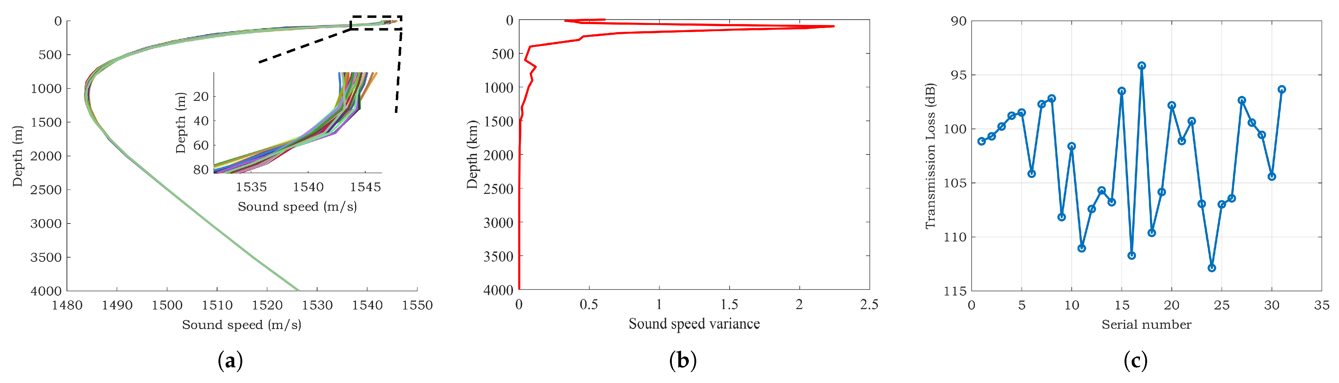
The TL is influenced by various factors, including actual oceanic environmental parameters, transmission depth, and reception depth. The variation of seawater properties across different temporal and spatial scales is substantial. For example, Figure 1a shows the average daily sound speed profile in a specific sea area during a particular month which was read from the HYCOM Global Ocean Forecasting System 3.1 [24] and Figure 1b is the variance in the sound speed at each depth. It illustrates significant disturbances in the surface layer of the deep-sea sound channel. This inherent complexity leads to an uncertain distribution of the underwater acoustic field. As shown in Figure 1c, the sound Transmission Loss (TL) values at a receiver 100 km away were obtained using the Range-dependent Acoustic Model–Parabolic Equation (RAM-PE) [25], based on the sound speed profile data shown in Figure 1a. The fluctuation in TL exceeds 20 dB, significantly impacting applications such as underwater communication performance prediction, sonar detection, and navigation [26]. In situations where environmental parameters change rapidly relative to the speed of sound propagation in water, such as long-range hydroacoustic communications, an underwater acoustic system that relies solely on deterministic environmental parameter models without considering environmental uncertainties may lead to significant disparities between predicted outcomes and actual results. This can compromise the accuracy and reliability of performance predictions. This paper primarily focuses on typical deep-sea environments, investigating the effects of uncertainties in marine environmental parameters such as sound speed profiles, seabed topography, and sediment layer properties on the TL. With the PDFs of marine environmental parameters, the objective is to calculate the TL PDF.
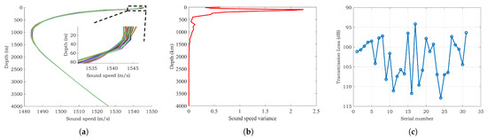
Figure 1.
(a) Perturbations in the sound speed profile. (b) The variance of the sound speed at each depth. (c) Fluctuations in transmission loss at 100 km due to perturbations in the sound speed profile.
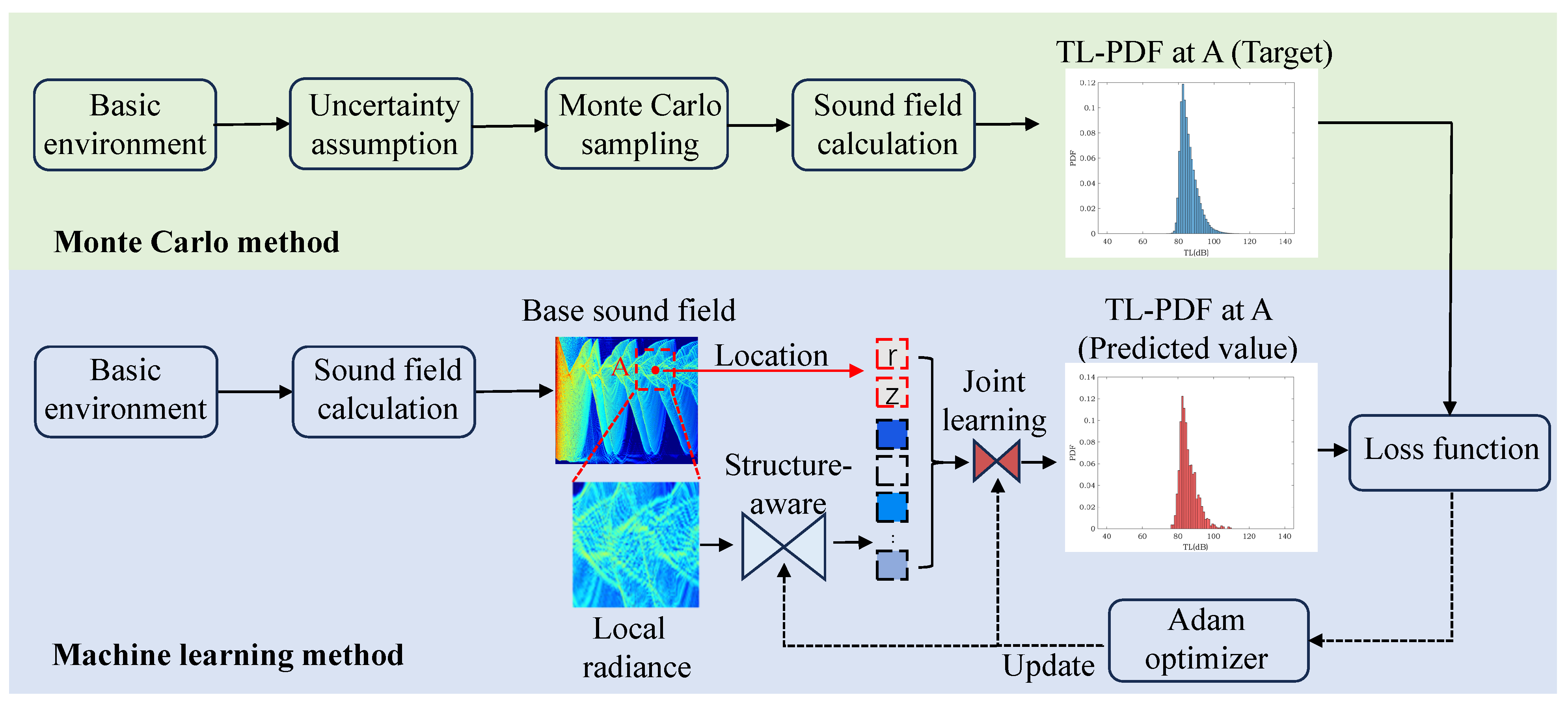
Figure 2 illustrates the proposed machine learning-based strategy for predicting TL’s uncertainty. In the proposed approach, the prediction problem of TL PDF is framed as a supervised regression task within the realm of machine learning. The proposed method has two key components: first, training labels are derived using the Monte Carlo method, and then a suitable machine learning model is designed to learn the correspondence between marine environment parameters obeying probability distributions and the TL PDF.
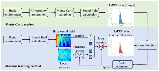
Figure 2.
Overall framework of the proposed machine learning method for estimating the TL PDF.
The Monte Carlo method, despite its computational intensity, serves as a valuable tool for algorithm validation due to its ease of implementation and inherent sampling randomness. The initial step involves using the Monte Carlo method to obtain the reference TL PDF, which is then employed as training labels. The specific procedure entails initially determining the best estimate of the true environmental characteristics for a given location and date from an available database, serving as the basic environment. Subsequently, the uncertainty in the marine environment is quantified, followed by the application of Monte Carlo principles to stochastically sample uncertain underwater acoustic parameters. This results in diverse parameter realizations. These realizations are then input into the acoustic field-propagation model, generating a range of acoustic field outcomes and facilitating the derivation of TL PDF.
In the design of neural networks, a sound field-calculation model is initially used to compute the TL field corresponding to the basic environment. For a given sound source parameter, the receiver and its associated local radiance can uniquely determine the oceanic environmental parameters in the basic environment, inspired by the matching field-processing technique [27]. Therefore, both the receiver and its corresponding local radiance are utilized as inputs to the neural network. The output of the neural network is the prediction of the TL PDF at that specific receiver. Subsequently, an appropriate loss function is devised to quantify the difference between the reference PDF and the PDF projected by the machine learning model. This difference will be diminished through an optimizer that updates the parameters within the machine learning model, narrowing the gap between the predicted PDF from the machine learning model and the reference PDF, until convergence is achieved.
3. Machine Learning Model
3.1. Specifics of the Model Input: The Position of the Receiver and Environmental Information
For a neural network to predict the TL PDF at a particular receiver, it is necessary to provide the following two pieces of information as inputs: marine environmental data and the position of the receiver. In this study, various oceanic environmental parameters are considered, including sound speed profile, seabed topography, and properties of sediment layer. These oceanic environmental parameters exhibit varying data formats under different measurement and spatial conditions. For instance, the quantity of sound speed profile data, which are composed of sound speed from different ocean depths, varies based on changes in maximum ocean depth and the measurement density of hydrographic databases. Similarly, the quantity of seafloor topography data, derived from the depths at various locations along a survey line, fluctuates with alterations in the maximum survey distance and the resolution of hydrographic databases.
Each input port of the neural network should correspond to an element in the prediction vector and maintain stability in its physical interpretation, remaining unaffected by changes in the input data. Consequently, if oceanic environmental parameters were to be directly utilized as the prediction vector for the neural network, the dimensionality of the prediction vector would need to adapt to the alterations in the data formats of these parameters. This would render it challenging to align the neural network’s input ports with a fixed physical interpretation. Directly incorporating oceanic environmental parameters as input ports for the neural network appears to be an impractical approach.
The approach undertaken in this study involves utilizing a sound field-calculation model to compute the TL field of the basic marine environment. Given sound source parameters, the basic marine environment is characterized by the position of the receiver, as well as the TL field surrounding that receiver, which is referred to as the local radiance. So our design diverges from directly utilizing marine environment parameters as model inputs. Instead, a sound field-computation model is employed to derive the sound field corresponding to the marine environment parameters. Subsequently, a local sound field around the receiver is selected. This local sound field is then employed as an indirect representation of marine environment parameters, serving as a part of the input for the machine learning model.
3.2. The Particular Structure of the Model
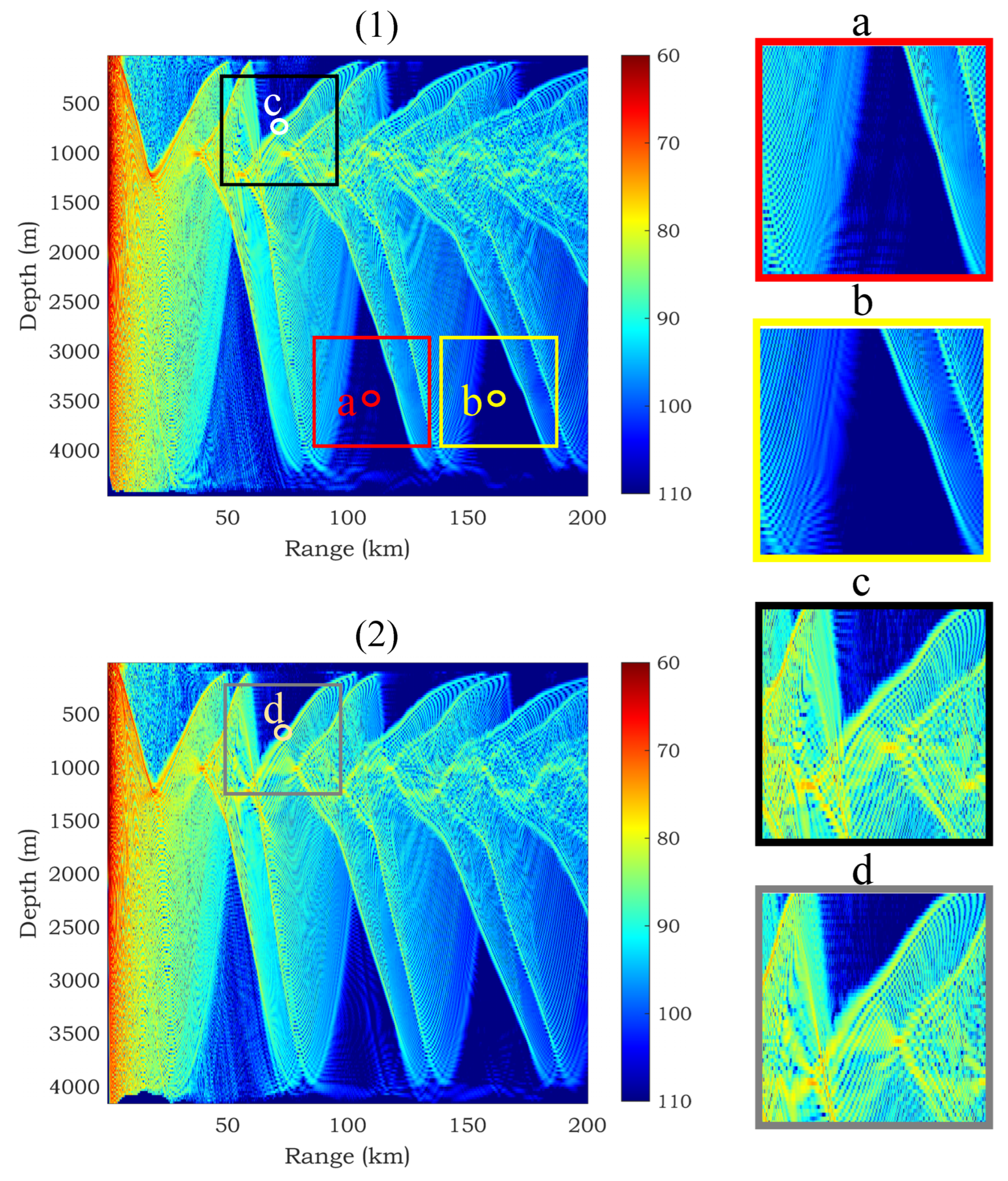
The schematic diagram of the local radiances of different receivers in the same basic environment and the local radiances of the same receiver in different basic environments is shown in Figure 3. While the local radiances of different receivers within the same basic environment or the local radiances of the same receiver in different basic environments exhibit significant numerical resemblance, there still exist structural discrepancies. The MLP network struggles to discern the subtle distinctions within these data structures, leading to diminished predictive performance in these specific regions. In light of this observation, a spatially informed network is developed in this paper to tackle this challenge. The comprehensive design of the network is illustrated in Figure 4.
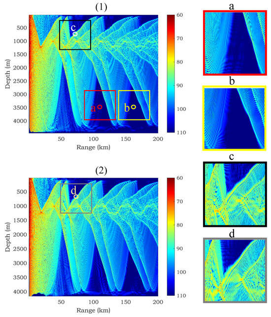
Figure 3.
Schematic diagram of different local radiances: (1) and (2) are the TL fields corresponding to two different basic environments; (a,b) two different receivers located in the TL field of the same basic environment; (c,d) the same receiver located in the TL fields of different basic environments.
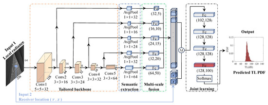
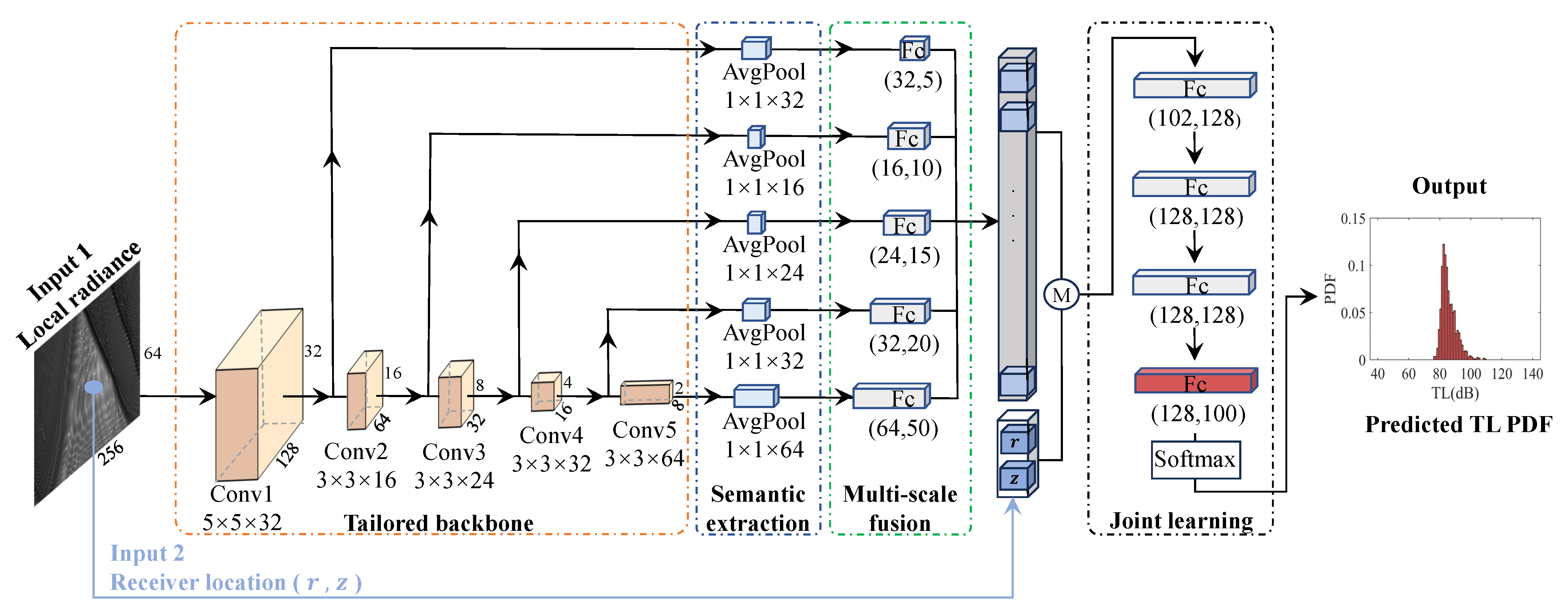
Figure 4.
Structure of the proposed machine learning model for prediction of a TL PDF.
Tailored backbone: Considering the exceptional capability of Convolutional Neural Networks (CNNs) in capturing local information and recognizing spatial patterns within data, a tailored backbone is proposed to capture the structural differences among different local radiances. These convolutional layers perform convolution operations on the input data by sliding convolution kernels across each position, effectively capturing local information within the local radiances. Subsequently, through the gradual stacking of multiple convolutional layers, feature information is progressively extracted and abstracted from the input data. This tailored backbone enhances the understanding of the data’s spatial structure within the local radiances, enabling a more precise analysis of subtle distinctions among different local radiances. The changing law of the number of channels of each convolutional layer refers to the architecture of MobileNet-Tiny [28].
Semantic extraction: Each convolutional layer possesses distinct receptive fields and channel numbers, enabling it to capture local information from the sound field-propagation image at various scales. The initial convolutional layer extracts fundamental features such as edges and textures from the original sound field-propagation image, while deeper convolutional layers progressively abstract higher-level semantic features. The feature maps obtained from each convolutional layer have varying spatial dimensions due to differences in the inputs and the sizes of receptive fields. Global average pooling (AvgPool) is primarily employed on the feature maps of each convolutional layer to reduce their spatial dimensions to 1 × 1 while preserving essential information from each channel [29]. This uniform spatial dimensionality facilitates subsequent multi-scale fusion, combining information from different scales for a more comprehensive understanding of the sound field-propagation image.
Multi-scale fusion: Finally, the integration of multiscale content from every semantic extraction layer is realized by employing a fully connected layer. Each convolutional layer specializes in distinct scales and intricate details. This process of multiscale fusion enables the global amalgamation of feature maps obtained from various scales across all convolutional layers, resulting in a comprehensive feature vector capable of depicting local radiance. Furthermore, this feature vector, in conjunction with the receiver’s location information, is processed through the subsequent layers of the neural network to accomplish specific tasks.
Joint learning: The features extracted through semantic extraction and multi-scale fusion from the local radiance are combined with the second part of the input information to implement joint learning. The second part of the input information pertains to the position of the receiver, including both the horizontal distance r of the receiver from the sound source and the vertical depth z of the receiver from the sea surface. The final regression task is performed by a deeper MLP to integrate and manipulate the advanced features extracted from the local radiance, along with the positional information of the receiver.
The output layer of the joint learning utilizes the softmax activation function to transform the model’s output into a probability distribution. This resulting probability distribution represents the predicted TL PDF obtained at a certain receiver by the model.
3.3. Loss Function
A loss function is utilized to quantify the dissimilarity between predictions generated by a machine learning model and the actual observations. Its primary function is to steer the adjustment of the machine learning model’s parameters in a manner that minimizes the loss function’s value. This iterative process assists the model in achieving a better fit with the training data and enhancing its ability to generalize to previously unseen data.
Denoting the PDF derived from the Monte Carlo method as y and the PDF predicted by the machine learning model as , Total Variation (TV) distance is employed to quantify the difference between the predicted PDF and the reference PDF [30].
where n is the length of the discrete PDF. The TV distance is used as a loss function, which quantifies the difference in area between two PDFs and is constrained within the range of 0 and 1. When , the PDF predicted by the machine learning precisely aligns with the reference PDF. Conversely, when , there is no overlap between the predicted and reference PDFs.
4. Dateset Construction and Division
The historical hydrographic environment of a certain sea area was utilized to construct a dataset through which the method and model proposed in this paper can be verified. When the application scope expands to include different descriptions of environmental properties or uncertainties, a new dataset can be created to retrain the machine learning model for deployment based on the new scenario.
4.1. The Process of Dataset Construction
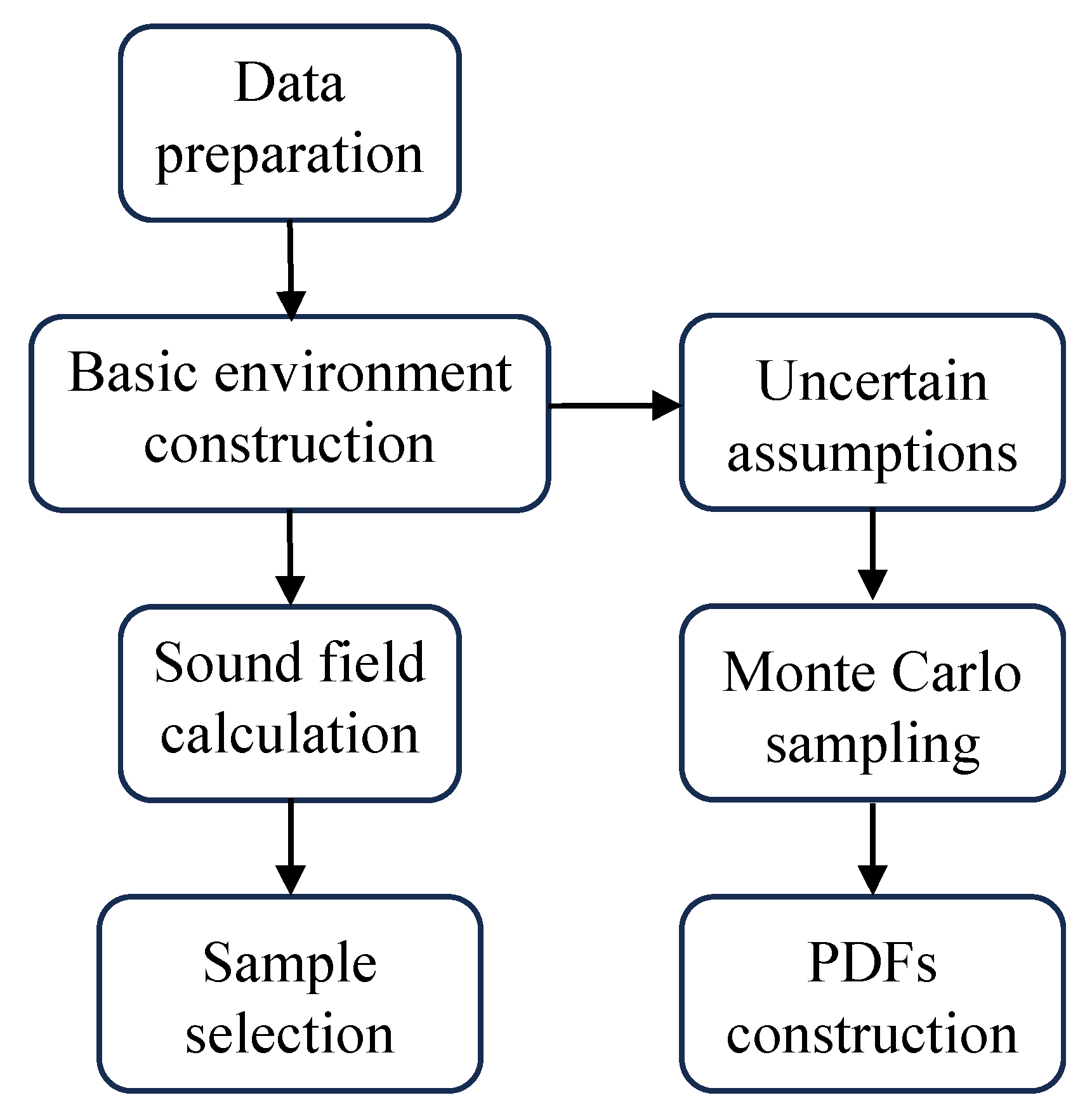
Figure 5 is a schematic diagram illustrating the steps involved in dataset construction. Initially, multiple sets of basic environment are selected from an available database. Subsequently, the obtained basic environmental data are used with a sound field-calculation model to derive the corresponding TL fields. By selecting specific sample receivers and their corresponding local radiances within the TL fields, the positions of these sample receivers and their local radiances are utilized as the input features for the machine learning samples. Simultaneously, by making uncertainty assumptions about the parameters in the basic environment and conducting Monte Carlo experiments, the TL PDFs at the receivers are obtained as the supervision label for the machine learning samples.
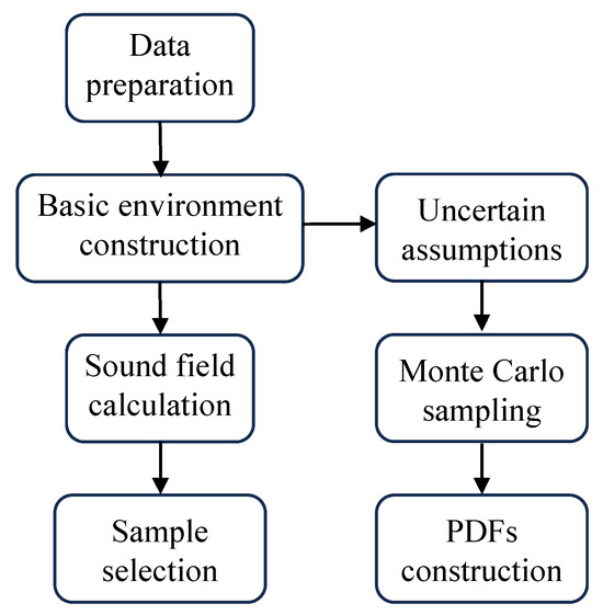
Figure 5.
Schematic diagram of the dataset-construction process.
Data preparation: The database used in this paper is the hydrological environment database of a typical deep-sea area in the South China Sea, which is approximately km2. This comprehensive database encompasses diverse parameters, including seabed topography, sediment layer characteristics, and seawater properties such as temperature and salinity. Seabed topography data boast a spatial resolution of in both latitude and longitude. Simultaneously, sediment layer data exhibit a resolution of in latitude and longitude. The temperature and salinity data are compiled as daily averages over the course of a specific month. These data points have a spatial resolution of in latitude and longitude. Within the database, values for temperature and salinity are assigned to various depths within the seawater column, where i represents the depth sequence number. Under general ocean conditions, Del Grosso proposed the following formula to convert temperature and salinity into a sound speed profile [31].
Basic environment construction: The process of selecting the basic environment from the database involves several steps. Firstly, a random set of latitude and longitude coordinates is assigned to the sound source. Based on the specified geographic coordinates, the average temperature and salinity data for the corresponding location are retrieved from the database. These values were then converted into the sound speed profile using Equation (3). Subsequently, a random azimuth angle is selected, and using the designated sound source as the starting point, a survey line is determined according to the chosen azimuth angle. Long-range sound fields are more significantly influenced by uncertain environmental characteristics compared to short-range ones, and the investigation of uncertainty in long-range sound fields holds great practical significance. Therefore, the maximum range for each survey line is assumed to be 200 km. From the database, the bathymetry along this survey line is extracted. Lastly, sediment layer parameters including sound speed c, density , and attenuation coefficients are obtained from the database at the geographic location in question. The derived sound speed profile, together with the bathymetry of the survey line and the parameters of the sediment layer, constitutes a comprehensive set of basic environment. This entire process is repeated 120 times to create a collection of 120 distinct basic environments. Figure 6 illustrates a representative example of a basic environment generated through the aforementioned methodology.
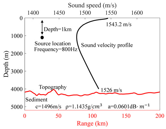
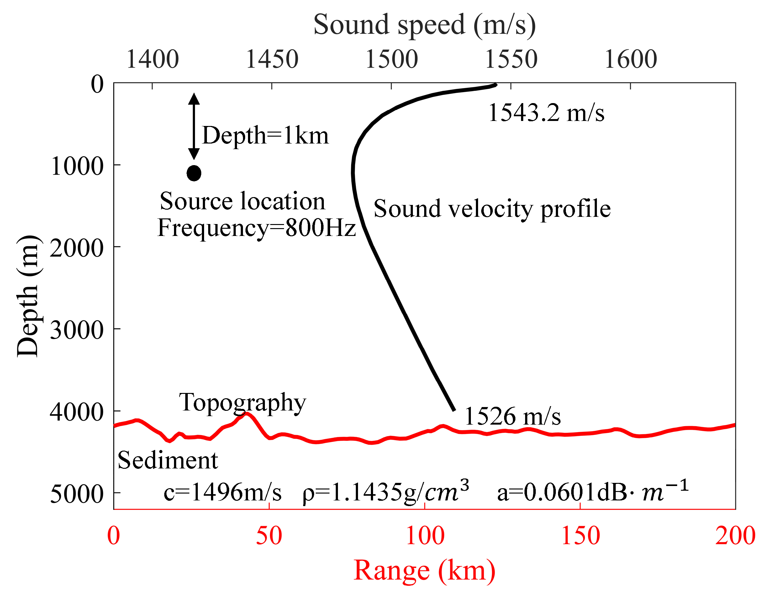
Figure 6.
A set of marine environmental parameters randomly selected from the available database.
Sound field calculation: The subsequent step involves the transformation of the basic environment into the receiver locations and the local radiance. The Range-dependent Acoustic Model-Parabolic Equation (RAM-PE) [25] serves as a commonly employed computational model for acoustic field simulations. Within the RAM-PE solver, the TL field corresponding to each basic environment is computed for a given consistent source frequency and source depth.
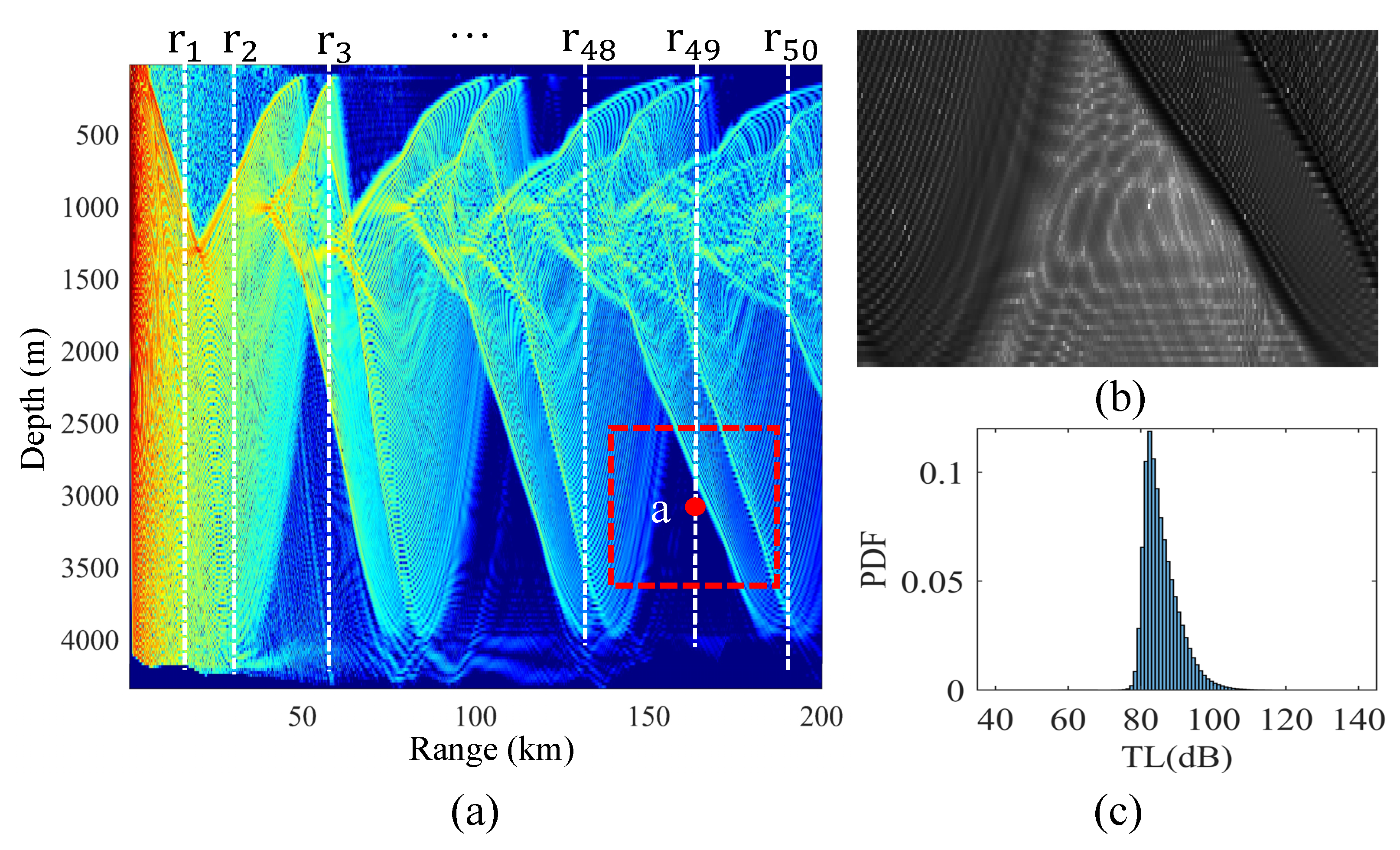
Sample selection: The first part of the input features of the sample is the location of the receiver. The selection process for these receivers is illustrated in Figure 7a. Fifty distances are randomly selected, with a sea depth resolution of 20 m at each distance. The horizontal distance r and vertical depth z of each sample receiver form a part of the sample input feature. The second component of the sample input feature is the local radiance associated with each receiver. The local radiance is composed of the TL values from neighboring receivers in the vicinity of the sample receiver. Figure 7b is the local radiance corresponding to the sample receiver a.
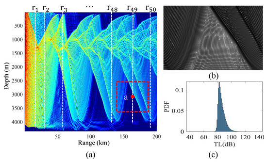
Figure 7.
The input features and label of one sample. (a) Method for selecting sample receivers (the White dotted line) and local radiances (the dotted box). (b) Local radiance represented as a grayscale image. (c) TL PDF at sample receiver a, obtained through the Monte Carlo method.
Uncertain assumptions: The sound speed profile is composed of the sound speeds at different depths of the sea water. The sound speeds at different depths within the sound speed profile exhibit a specific relationship. Consequently, when introducing uncertainty assumptions for the sound speed profile, it is inappropriate to treat the sound speed at each depth as independent and identically distributed. Following the methodology outlined in [32], an empirical orthogonal decomposition is first performed on the sound speed profiles at each geographic location. This process extracts the first few empirical orthogonal coefficients (EOCs) that account for 99% of the variance. Subsequently, the distribution of the EOCs is employed as a surrogate for the distribution of the sound speed profile.
The uncertainty in seafloor topography arises primarily from limitations in measurement technologies and algorithms. For deep-sea regions constrained by satellite altimetry, the estimated uncertainty of water depth within each grid unit is ±150 m [33]. The uncertainty in seafloor topography in this paper is modeled under the assumption that the error in each depth measurement follows a normal distribution with a mean of zero and a variance of 150.
The parameters of sedimentary layers are challenging to obtain directly through measurements and are typically derived via inversion using matched field-processing techniques. The primary source of uncertainty in sedimentary layer parameters arises from errors associated with matched field processing [34]. For uncertainty modeling, the error in sound velocity is assumed to follow a normal distribution with a mean of zero and a variance of 5% of the measured value. Similarly, the error in density is modeled as a normal distribution with a mean of zero and a variance of 5% of the measured value, while the error in the attenuation coefficient is described by a log-normal distribution with a mean of zero and a variance of 5% of the measured value [35].
Monte Carlo sampling: Once the uncertainties are assumed for each marine environmental parameter in the baseline environment, the next step involves utilizing the Monte Carlo Sampling (MCS) method to extract experimental sample points from the space of random marine environmental parameters.
PDF construction: Figure 7c depicts the TL PDF at sample receiver a, obtained using the Monte Carlo. The Monte Carlo experiments are performed to obtain the TL PDFs by sampling the distributions obeyed by the parameters in the baseline environment through the aforementioned MCS method. This leads to acquiring 1000 uncertainty realizations for each baseline environment. Subsequently, the RAM-PE solver is used to calculate the TL field corresponding to each uncertainty realization of the environment. This process yields 1000 TL values at each sample receiver within each baseline environment. These 1000 TL values at each sample receiver are then combined into histograms containing 100 bins.
4.2. Division of Training and Testing Datasets
As shown in Section 4.1, 120 groups of basic environments were randomly selected from the sea area of the available database. A number of receivers and their surrounding TL fields were then randomly selected among the sound fields corresponding to each group of basic environments computed by the sound field computational model RAM-PE. A receiver and its surrounding TL field then constitute the input features of a sample. The number of randomly selected sample receivers in the sound field corresponding to each group of basic environments is about , so a total of 1,285,863 samples are generated in 120 groups of basic environments. The dataset composed of the samples in the 120 groups of basic environments is divided into a training dataset and a test dataset. The training dataset contains 1,089,000 samples in the 100 groups of basic environments, and the training dataset contains 196,863 samples in the 20 groups of basic environments.
After completing the model training, its predictive performance is evaluated using the samples in the test dataset. The purpose of the test is to evaluate the model’s ability to predict TL PDFs of sample receivers in a sound field corresponding to a basic environment that has not been encountered before. Therefore, all sample receivers in each group of the basic environment are treated as a test subset, resulting in a total of 20 test subsets.
5. Experiments
5.1. Implementation
The neural network training process, implemented with PyTorch 2.0, involves adjusting parameters to minimize loss function by calculating gradients and using a optimizer. The local radiance uses a grid size of 256 × 64, covering a distance of 52.2 km and a depth of 1280 m, matching the acoustic shadow zone. During training, hyperparameter tuning was carried out. The number of convolutional layers and the size of each convolutional layer in the tailored backbone network, the parameters of the linear layers in the multi-scale fusion and the joint learning are all illustrated in Figure 4. Additional system parameters when training the SICNet can be found in Table 1. The process of training the SICNet model is shown in Algorithm 1.
| Algorithm 1 Training SICNet via Forward and Backward Propagation |
|

Table 1.
Some system parameters when training the SICNet.
The Monte Carlo-derived TL PDF was used as the reference benchmark. The following statistical methods designed for distribution comparison are applied to gauge the accuracy of the proposed machine learning-based TL PDF prediction model. These methods enable a comprehensive and precise analysis for effective comparison of the predicted TL PDF with the Monte Carlo-generated PDF to identify disparities. In addition to the TV distance introduced in Section 3.3, another statistical method is used to quantify the dissimilarity between two PDFs, denoted as and . These two metrics are applicable in different situations. It is necessary to select the appropriate metric based on the specific problem. This paper employs these metrics to not only ease the assessment of SICNet’s prediction accuracy, but also as a benchmark for comparing prediction performance among different methods.
Kolmogorov–Smirnov (KS) test: The KS test [36] assesses similarity between probability distributions by establishing a null hypothesis, calculating the maximum difference statistic D (also called the KS statistic), and determining the critical value p based on statistic D and sample size n. If at significance level , the null hypothesis is accepted, indicating identical probability density functions. Otherwise, it is rejected. A commonly accepted significance level in statistics is = 0.05 [37].
where and are the cumulative distribution functions of the first PDF and the second PDF , respectively. Designed to compare differences between two cumulative distributions, the KS test provides an accurate measure of the gap with the KS statistic (larger values indicate greater dissimilarity between the two distributions). Nonetheless, the approach solely indicates differences and does not provide an evaluation of the similarities between the distributions.
5.2. Experimental Results
5.2.1. Performance Analysis
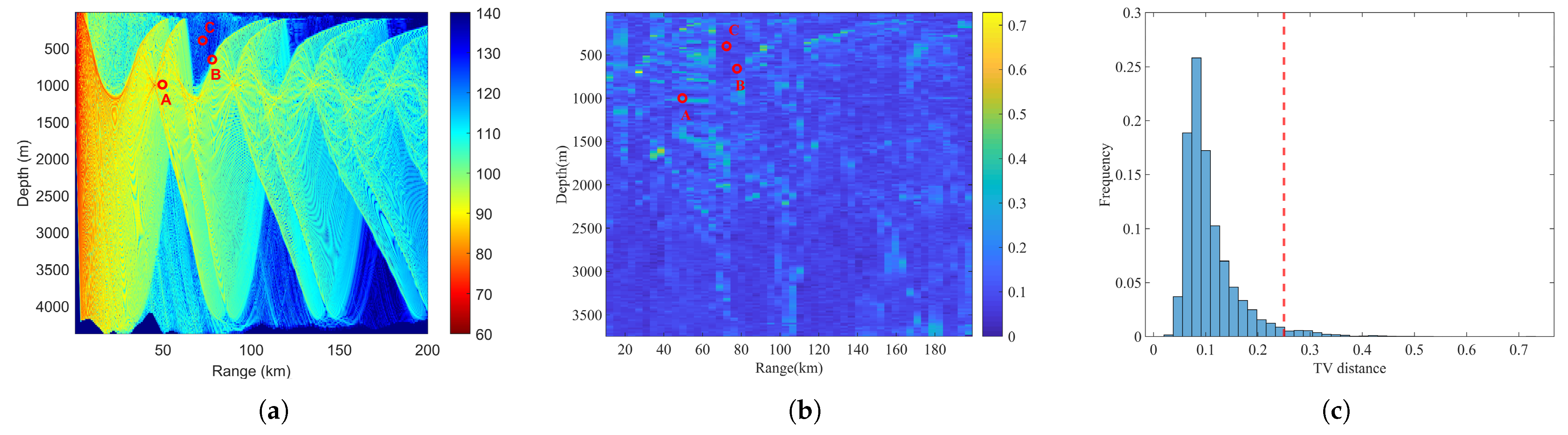
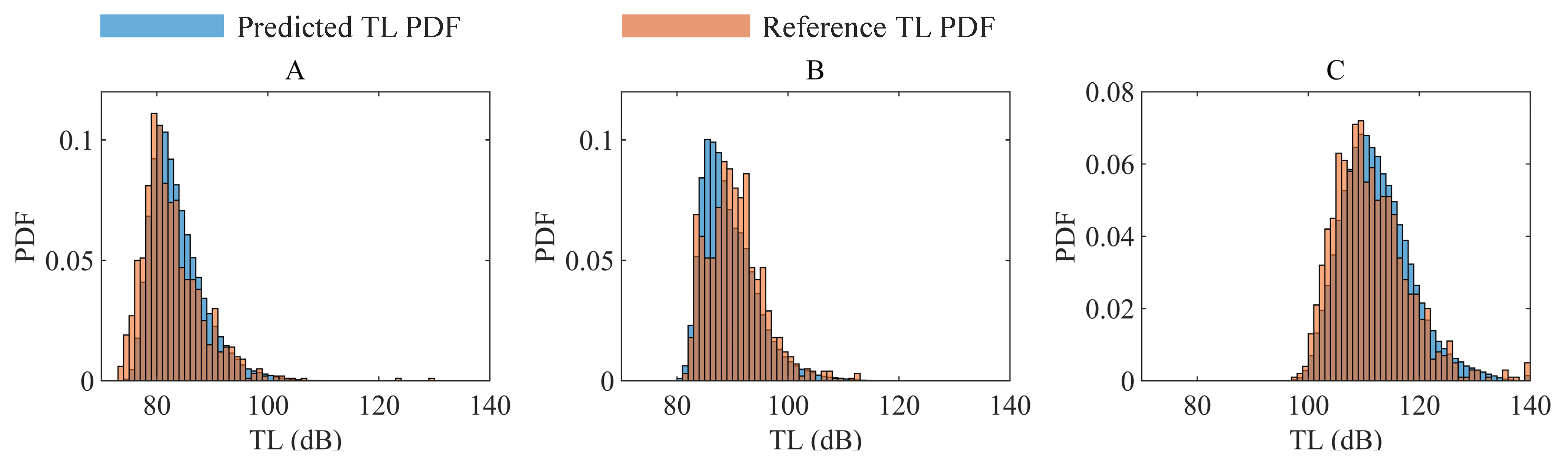
Accuracy assessment: Figure 8 presents the TV distance between predicted and reference TL PDFs in a specific test subset of 9984 samples. The average TV distance is 0.1018. The TV distance value up to 0.25 indicate converged-to-approximate PDF matching within engineering accuracy, as a TV distance of 0.25 typically corresponds to a standard deviation error of up to 2 dB [9]. The percentage of receivers that exceed this threshold 0.25 in this test subset is 97.11%. Figure 9 illustrates the predicted TL PDF and the TL PDF obtained through Monte Carlo simulations for the three receivers depicted in Figure 8a,b. Point A is located in the convergence area, point B in the transition area, and point C in the shadow area. It is observed that the TL at point A in the convergence area is the smallest and most concentrated, while the TL at point C in the shadow area is the largest and most dispersed. At all three points in these distinct regions, the PDF predicted by the SICNet model closely resembles the PDF obtained through Monte Carlo simulations. Moreover, at a 0.05 significance level, KS tests show that 97.63% of the samples confirm similarity between the proposed method’s TL PDF predictions and the traditional Monte Carlo method’s.

Figure 8.
(a) TL field corresponding to a basic environment and A, B, C are three different receivers. (b) The TV distance between the TL PDF at each receiver predicted by the SICNet model and the TL PDF obtained through Monte Carlo simulation, with uncertainty introduced into the parameters of the basic environment. (c) Statistical analysis of the TV distances for all sample receivers in the basic environment. The red dotted line shows the TV distance threshold of 0.25.
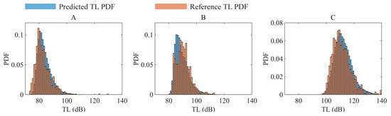
Figure 9.
TL PDFs predicted by the SICNet network and Monte Carlo simulation at three distinct receivers. The TV distances at the A, B, C receivers are 0.14, 0.16, 0.10, respectively.
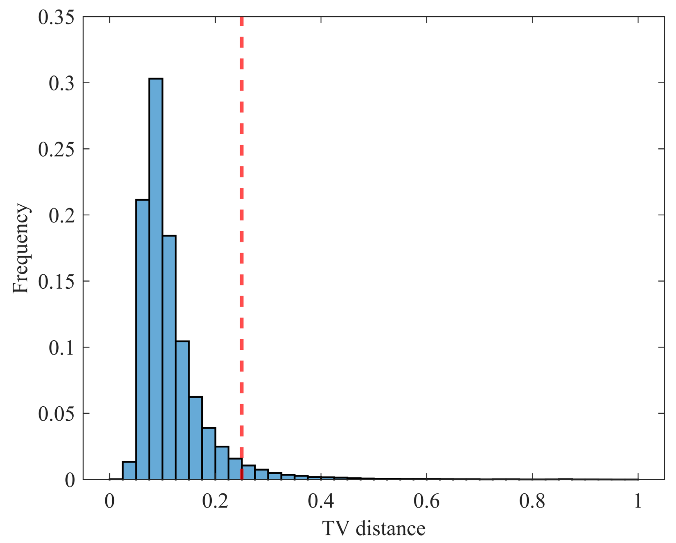
A statistical analysis is also performed on the TV distance for all testing samples, comprising a total of 196,863 test samples across 20 testing subsets. Figure 10 presents the statistical results of the TV distance for all samples. The average TV distance is 0.1166, and 95.92% of the samples exhibit a TV distance below 0.25. The overall average TV distance for all samples is 0.1948. The KS test is also conducted at the 0.05 significance level, with results indicating that 94.98% of the samples validate the similarity between the proposed method’s predicted TL PDF and the traditional Monte Carlo method’s TL PDF.

Figure 10.
Histogram statistics of TV distance for 196,863 test samples. The red dotted line shows the TV distance threshold of 0.25.
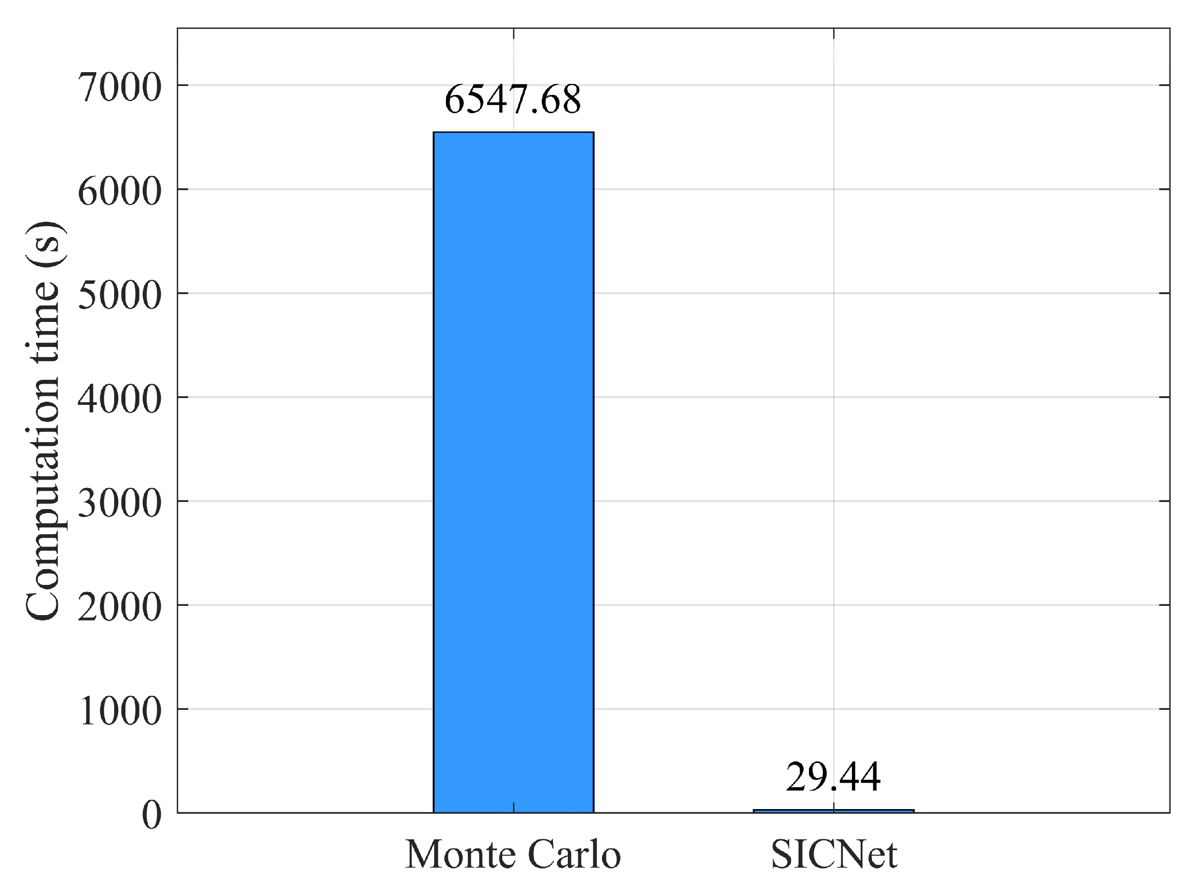
Efficiency comparison: When the offline training of the model is completed, a new baseline environment is obtained from the database, and then the TL PDFs at the receivers are obtained using the Monte Carlo method and the proposed method, respectively. The comparison of the time required for each of these two methods to predict TL PDFs online in practical applications is performed. Figure 11 compares the computational efficiency of the traditional method and the proposed method.
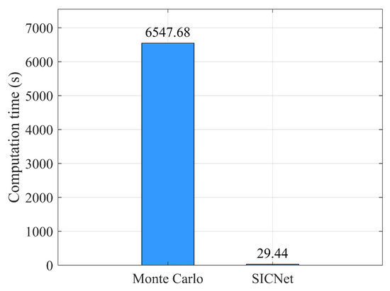
Figure 11.
The time required to calculate the PDF of TL in practical applications using the Monte Carlo method versus the proposed method.
The use of the Monte Carlo method requires iterative calls to the sound field computational model RAM-PE, which is a FORTRAN code based on the latest parabolic equation technique. TL PDFs at each receiver are obtained by calling the RAM-PE model 1000 times on MATLAB 2019a, and the whole process took 6547.68 s. In the proposed method, the RAM-PE model is first invoked once in MATLAB to acquire the sound field corresponding to the basic environment. This process takes 6.4 s. Next, the trained SICNet model is loaded on PyTorch 2.0 and tested to obtain the TL PDFs of the receivers, with this step taking 29.44 s. The total time for obtaining the TL PDFs at the receivers using the SICNet is 35.84 s, demonstrating a computational efficiency improvement of two orders of magnitude compared to the traditional Monte Carlo method. Both MATLAB and PyTorch 2.0 were run on the same Windows computer with an X64 processor.
Impact of data resolution: The ocean environment is modeled as the location of the receiver and the surrounding local TL field, which is used as the input to the SICNet model. As shown in Figure 4, the features in the local TL field are first extracted by the SICNet model, followed by joint learning with the location of the receiver. Three different data resolutions for the local TL image in terms of depth and distance are designed, namely 20 m × 200 m, 40 m × 400 m, and 80 m × 800 m. Figure 12 illustrates the changes in the local TL image, covering the same depth and distance range, under different data resolutions. Subsequently, the SICNet model was trained using datasets constructed under different data resolutions. The TV distance distribution diagram of the TL PDF, predicted by the model trained with datasets of different resolutions in the same set of basic environments, is shown in Figure 13. The average TV distances of the TL PDF predicted by the models at three different resolutions (20 m × 200 m, 40 m × 400 m, and 80 m × 800 m) for the same basic environment are 0.10, 0.14, and 0.17, respectively. It can be observed that a higher resolution in the local sound field leads to better prediction performance of the model. The resolution of the local sound field in distance and depth has a significant impact on the model’s performance. Higher resolution images of the local sound field contain richer features, which provide more structural information to the model, thereby facilitating the model’s feature extraction of the local sound field.
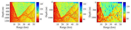
Figure 12.
Changes in the TL image of the same local sound field at different data resolutions. From left to right, the distance and depth resolution of TL are 20 m × 200 m, 40 m × 400 m, and 80 m × 800 m, respectively.
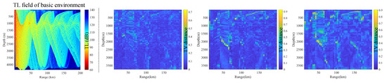
Figure 13.
TV distance distribution of the TL PDF predicted by the SICNet model after training with different resolution datasets under the same set of basic environments (the left of the dotted line). The right side of the dotted line corresponds to the prediction performance of the SICNet model at data resolutions 20 m × 200 m, 40 m × 400 m, and 80 m × 800 m from left to right.
Model scalability: In constructing the dataset, the basic environments used for both training and testing were randomly selected from the same sea area outlined by the red box in Figure 14a. The model’s prediction performance for environments outside this area, such as the survey line AB shown in Figure 14a, is presented in Figure 14d. The average TV distance predicted by the model for the TL PDF corresponding to this external environment is 0.1188. This value differs by only 0.017 from the average TV distance of 0.1018 predicted by the model within the training area, as depicted in Figure 8. When the model encounters an unfamiliar environment with hydrological conditions similar to those of the training sea area, it continues to demonstrate strong prediction performance. This indicates that the SICNet model exhibits a degree of scalability.
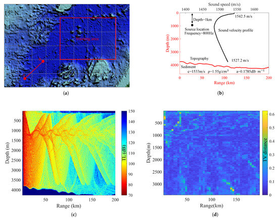
Figure 14.
(a) The sea area used for model training and the survey line AB for scalability testing. (b) Various parameters of the basic environment corresponding to the survey line AB. (c) TL field calculated based on the basic environment corresponding to the survey line AB. (d) TV distance distribution of the TL PDF predicted by the SICNet model on line AB.
5.2.2. Performance Comparison
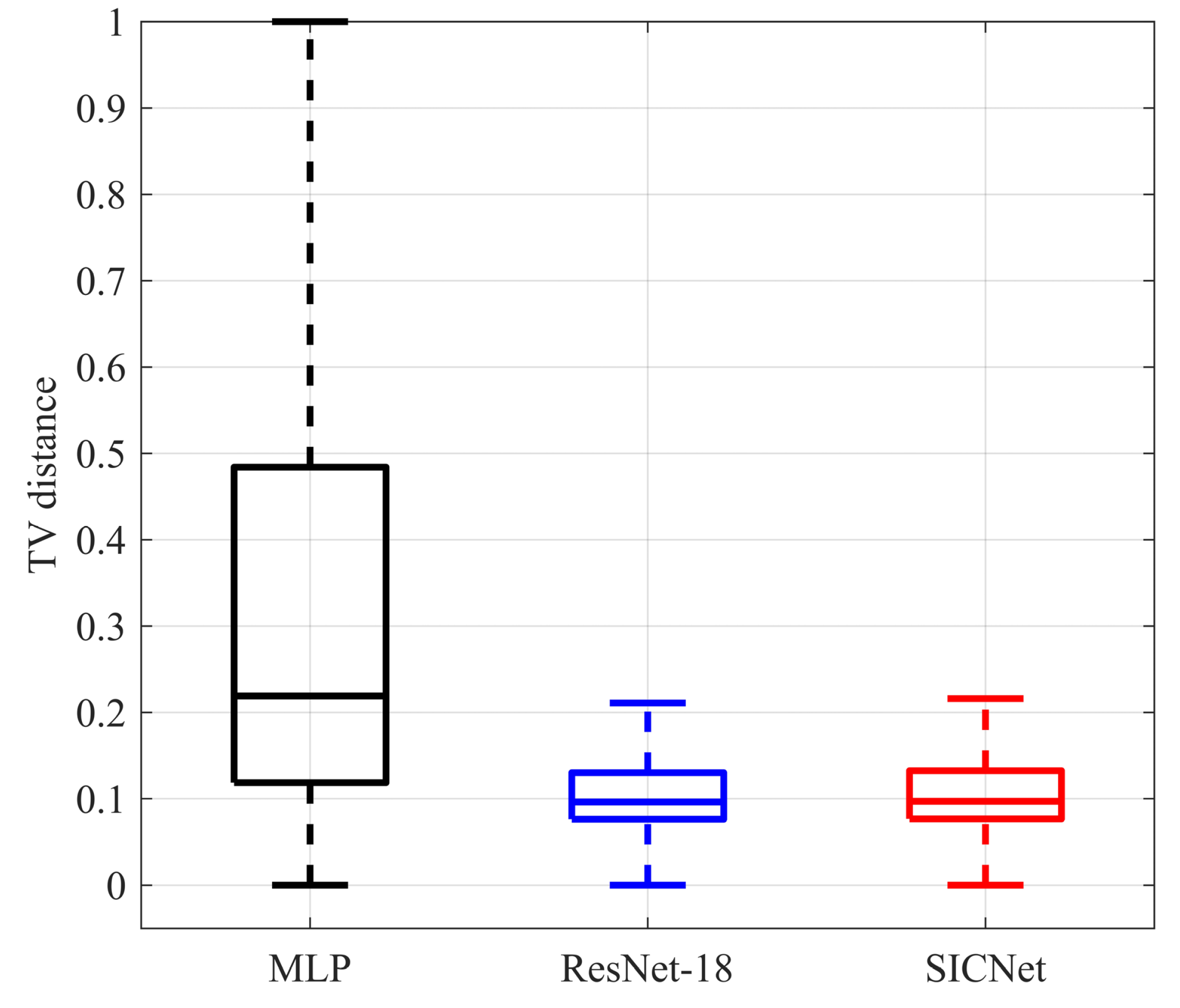
In contrast to prior work that employed a straightforward MLP network combining local radiance and receiver locations [19], SICNet takes a distinct approach by decoupling these elements. A convolutional neural network is initially employed to extract features from local radiance, and these features are subsequently integrated with receiver locations. To assess the efficacy of the tailored backbone network, semantic extraction, and multi-scale fusion components in SICNet, they are substituted with ResNet-18, a well-established deep CNN architecture [38]. Table 2 provides a comparative analysis of MLP, ResNet-18, and SICNet from two perspectives: first, in terms of KS test similarity and average TV distance for TL’s PDF prediction performance across all samples; and second, in terms of evaluating model parameters and sizes. Figure 15 presents a statistical analysis of TV distances for all samples across the three models, displayed in the form of box plots.
Table 2.
Comparison of prediction performance and model complexity of the three models.

Figure 15.
The statistical results of the TV distances of all samples in the test set predicted by the three models are displayed using box plots.
Table 2 and Figure 15 provide compelling evidence of the superior performance of SICNet and ResNet-18 when compared to MLP. This superiority is evident in terms of KS test similarity and TV distance. These results highlight the effectiveness of SICNet’s approach, which separates local radiation and receiver locations. By applying convolution to local radiance before jointly learning with receiver positions, it markedly enhances the model’s predictive capabilities for TL’s PDF. Moreover, in terms of model size, SICNet boasts model parameters and dimensions that are nearly half the size of MLP and two orders of magnitude smaller than ResNet-18. In summary, the study shows that SICNet not only delivers superior performance but also offers a more compact model size compared to ResNet-18 and MLP.
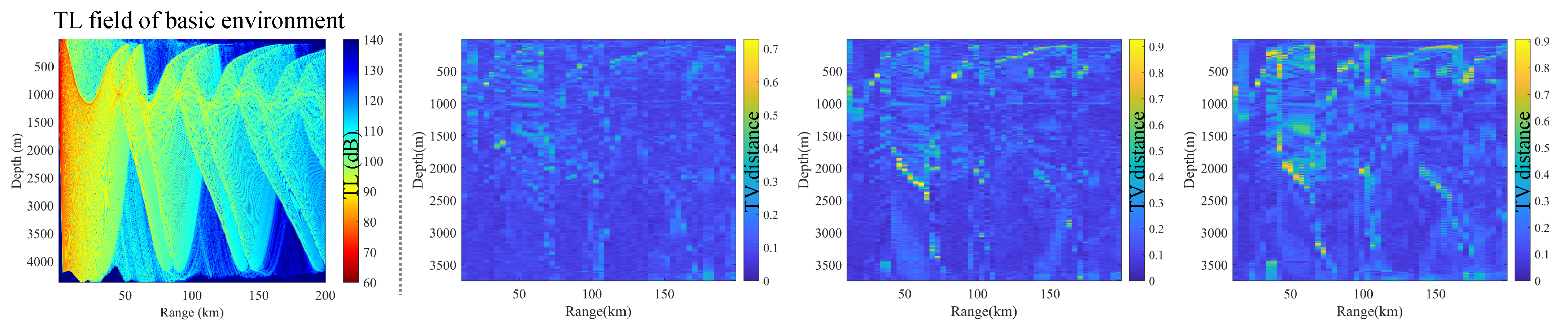
In Figure 16, the TV distance distribution on a test subsets reveals nuanced performance disparities. From the distribution of TV distances, the MLP network underperforms in shadow areas, while ResNet-18 and SICNet exhibit improved predictive performance. This improvement is attributed to their direct incorporation of local radiance as input to the convolutional neural network, facilitating effective extraction of local features within the radiance and superior discrimination of subtle differences among local radiances.
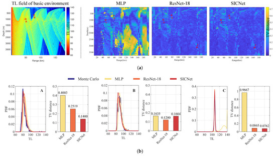
Figure 16.
(a) Predictive performance of three models on test subsets. (1) The TL field of a basic environment. (2) The TV distance between the TL PDFs predicted by the three models and that obtained using the Monte Carlo method. (b) Comparison of the TV distances between the TL PDFs predicted by each model and the TL PDF obtained using the Monte Carlo method at three distinct receivers A, B and C.
6. Conclusions
The dynamic ocean environment makes accurate sound-propagation prediction challenging. Rapid estimation of acoustic field uncertainty enhances underwater detection, communication reliability, marine resource exploration, and environmental monitoring. By providing probabilistic insights into TL, it enables optimized detection parameters, improving target recognition and signal processing. In environmental monitoring, it aids equipment deployment and informs monitoring strategies. A machine learning approach for assessing sound TL uncertainty is introduced in this paper. The intricate relationship between oceanic parameters and TL distribution is effectively modeled by the proposed spatially informed neural network. A specialized dataset was created using hydroacoustic data and the RAM-PE solver. Key findings, based on comprehensive experimental results, are summarized as follows:
(1) TL PDFs are effectively approximated by the proposed method compared to the Monte Carlo approach, offering significant computational efficiency. The proposed approach improves efficiency by two orders of magnitude compared to 1000 Monte Carlo simulations, demonstrating practical potential in various high real-time performance underwater acoustic applications.
(2) Addressing the challenge of modeling oceanic variables within machine learning, oceanic parameters are expressed as local radiances related to receivers. The proposed model overcomes limitations by employing convolution operations that effectively extract local features, significantly improving predictive performance, particularly within the shadow zone.
The effectiveness of the proposed method in deep-sea environments has been verified using the constructed dataset. Future research will focus on enhancing the applicability of the proposed method and improving model interpretability. Transferability will be improved through pre-training and data augmentation to address potential mismatches in more complex, unseen environments. The decision-making process will be analyzed by evaluating feature contributions and visualizing neural network focus areas, enhancing prediction transparency and reliability. Given the distinct sound-propagation characteristics and greater environmental variability of shallow waters, integrating physical acoustics with AI training strategies will help assess effectiveness in such conditions.
Author Contributions
Conceptualization, X.C. and H.W.; methodology, X.C.; software, X.C.; validation, X.C.; formal analysis, X.C.; investigation, C.L. and H.W.; resources, J.W., Y.T. and C.M.; data curation, C.L.; writing—original draft preparation, X.C.; writing—review and editing, C.L., Y.T., J.W., C.M. and H.W.; supervision, H.W. and C.M.; project administration, H.W.; funding acquisition, H.W. All authors have read and agreed to the published version of the manuscript.
Funding
The research was supported by the Chinese Academy of Sciences (XDB0700403) and the China Scholarship Council.
Institutional Review Board Statement
Not applicable.
Informed Consent Statement
Not applicable.
Data Availability Statement
The data that support the findings of this study are available from the Institute of Acoustics of the Chinese Academy of Sciences. Data are available from the authors upon request and with the permission of the Institute of Acoustics of the Chinese Academy of Sciences.
Acknowledgments
The authors would like to thank the editors and reviewers for their comments on the manuscript of this article.
Conflicts of Interest
The authors declare no conflicts of interest.
Abbreviations
The following abbreviations are used in this manuscript:
| TL | Transmission Loss |
| Probability Density Function | |
| SICNet | Spatially Informed Convolutional Neural Network |
| MLP | Multi-Layer Perceptron |
| ResNet-18 | Residual Network with 18 layers |
| TV distance | Total Variation distance |
| KS | Kolmogorov–Smirnov |
References
- Song, A.; Badiey, M.; Song, H.C.; Hodgkiss, W.S.; Porter, M.B. Impact of ocean variability on coherent underwater acoustic communications during the Kauai experiment (KauaiEx). J. Acoust. Soc. Am. 2008, 123, 856–865. [Google Scholar] [CrossRef] [PubMed]
- Sha, L.; Nolte, L.W. Effects of environmental uncertainties on sonar detection performance prediction. J. Acoust. Soc. Am. 2005, 117, 1942–1953. [Google Scholar] [CrossRef]
- Masetti, G.; Kelley, J.G.W.; Johnson, P.; Beaudoin, J. A ray-tracing uncertainty estimation tool for ocean mapping. IEEE Access 2017, 6, 2136–2144. [Google Scholar] [CrossRef]
- Kessel, R.T. A mode-based measure of field sensitivity to geoacoustic parameters in weakly range-dependent environments. J. Acoust. Soc. Am. 1999, 105, 122–129. [Google Scholar] [CrossRef]
- Metropolis, N. The beginning. Los Alamos Sci. 1987, 15, 125–130. [Google Scholar]
- Finette, S. A stochastic representation of environmental uncertainty and its coupling to acoustic wave propagation in ocean waveguides. J. Acoust. Soc. Am. 2006, 120, 2567–2579. [Google Scholar] [CrossRef]
- Hou, T.Y.; Luo, W.; Rozovskii, B.; Zhou, H.M. Wiener chaos expansions and numerical solutions of randomly forced equations of fluid mechanics. J. Comput. Phys. 2006, 216, 687–706. [Google Scholar] [CrossRef]
- Dosso, S.E.; Morley, M.G.; Giles, P.M.; Brooke, G.H.; McCammon, D.F.; Pecknold, S.; Hines, P.C. Spatial field shifts in ocean acoustic environmental sensitivity analysis. J. Acoust. Soc. Am. 2007, 122, 2560–2570. [Google Scholar] [CrossRef]
- James, K.R.; Dowling, D.R. A method for approximating acoustic-field-amplitude uncertainty caused by environmental uncertainties. J. Acoust. Soc. Am. 2008, 124, 1465–1476. [Google Scholar] [CrossRef]
- Roberts, P.L.; Jaffe, J.S.; Trivedi, M.M. Multiview, broadband acoustic classification of marine fish: A machine learning framework and comparative analysis. IEEE J. Ocean. Eng. 2011, 36, 90–104. [Google Scholar] [CrossRef]
- Lowell, K.; Hermann, J. Accuracy of bathymetric depth change maps using multi-temporal images and machine learning. J. Mar. Sci. Eng. 2024, 12, 1401. [Google Scholar] [CrossRef]
- O’Byrne, M.; Pakrashi, V.; Schoefs, F.; Ghosh, B. Semantic segmentation of underwater imagery using deep networks trained on synthetic imagery. J. Mar. Sci. Eng. 2018, 6, 93. [Google Scholar] [CrossRef]
- Niu, H.; Ozanich, E.; Gerstoft, P. Ship localization in Santa Barbara Channel using machine learning classifiers. J. Acoust. Soc. Am. 2017, 142, EL455–EL460. [Google Scholar] [CrossRef] [PubMed]
- Seo, D.; Lee, D.; Park, S.; Oh, S. Hyperspectral Image-Based Identification of Maritime Objects Using Convolutional Neural Networks and Classifier Models. J. Mar. Sci. Eng. 2024, 13, 6. [Google Scholar] [CrossRef]
- Shi, J.H.; Liu, Z.j. Deep learning in unmanned surface vehicles collision-avoidance pattern based on AIS big data with double GRU-RNN. J. Mar. Sci. Eng. 2020, 8, 682. [Google Scholar] [CrossRef]
- Niu, H.; Reeves, E.; Gerstoft, P. Source localization in an ocean waveguide using supervised machine learning. J. Acoust. Soc. Am. 2017, 142, 1176–1188. [Google Scholar] [CrossRef]
- Wang, D.; Zhang, Y.; Wu, L.; Tai, Y.; Wang, H.; Wang, J.; Meriaudeau, F.; Yang, F. Robust Underwater Acoustic Channel Estimation Method Based on Bias-Free Convolutional Neural Network. J. Mar. Sci. Eng. 2024, 12, 134. [Google Scholar] [CrossRef]
- Zhang, Y.; Wang, H.; Li, C.; Chen, D.; Meriaudeau, F. Meta-learning-aided orthogonal frequency division multiplexing for underwater acoustic communications. J. Acoust. Soc. Am. 2021, 149, 4596–4606. [Google Scholar] [CrossRef]
- Lee, B.M.; Johnson, J.R.; Dowling, D.R. Predicting Acoustic Transmission Loss Uncertainty in Ocean Environments with Neural Networks. J. Mar. Sci. Eng. 2022, 10, 1548. [Google Scholar] [CrossRef]
- Hu, J.; Shen, L.; Sun, G. Squeeze-and-excitation networks. In Proceedings of the IEEE Conference on Computer Vision and Pattern Recognition, Salt Lake City, UT, USA, 18–22 June 2018; pp. 7132–7141. [Google Scholar]
- Karpathy, A.; Toderici, G.; Shetty, S.; Leung, T.; Sukthankar, R.; Fei-Fei, L. Large-scale video classification with convolutional neural networks. In Proceedings of the IEEE Conference on Computer Vision and Pattern Recognition, Columbus, OH, USA, 23–28 June 2014; pp. 1725–1732. [Google Scholar]
- Krizhevsky, A.; Sutskever, I.; Hinton, G.E. Imagenet classification with deep convolutional neural networks. Adv. Neural Inf. Process. Syst. 2012, 25. [Google Scholar] [CrossRef]
- Gardner, M.W.; Dorling, S. Artificial neural networks (the multilayer perceptron)—A review of applications in the atmospheric sciences. Atmos. Environ. 1998, 32, 2627–2636. [Google Scholar] [CrossRef]
- Chassignet, E.P.; Hurlburt, H.E.; Smedstad, O.M.; Halliwell, G.R.; Hogan, P.J.; Wallcraft, A.J.; Baraille, R.; Bleck, R. The HYCOM (Hybrid Coordinate Ocean Model) Data Assimilative System. J. Mar. Syst. 2007, 65, 60–83. [Google Scholar] [CrossRef]
- Collins, M.D. A split-step Padé solution for the parabolic equation method. J. Acoust. Soc. Am. 1993, 93, 1736–1742. [Google Scholar] [CrossRef]
- Robinson, A.; Abbot, P.; Lermusiaux, P.; Dillman, L. Transfer of uncertainties through physical-acoustical-sonar end-to-end systems: A conceptual basis. In Impact of Littoral Environmental Variability of Acoustic Predictions and Sonar Performance; Springer: Berlin/Heidelberg, Germany, 2002; pp. 603–610. [Google Scholar]
- Baggeroer, A.B.; Kuperman, W.A.; Mikhalevsky, P.N. An overview of matched field methods in ocean acoustics. IEEE J. Ocean. Eng. 1993, 18, 401–424. [Google Scholar] [CrossRef]
- Sanjay, N.S.; Ahmadinia, A. MobileNet-Tiny: A deep neural network-based real-time object detection for rasberry Pi. In Proceedings of the 2019 18th IEEE International Conference On Machine Learning And Applications (ICMLA), Boca Raton, FL, USA, 16–19 December 2019; pp. 647–652. [Google Scholar]
- Lin, M.; Chen, Q.; Yan, S. Network in network. arXiv 2013, arXiv:1312.4400. [Google Scholar]
- Levin, D.A.; Peres, Y. Markov Chains and Mixing Times; American Mathematical Soc.: Washington, DA, USA, 2017; Volume 107. [Google Scholar]
- Del Grosso, V.A. New equation for the speed of sound in natural waters (with comparisons to other equations). J. Acoust. Soc. Am. 1974, 56, 1084–1091. [Google Scholar] [CrossRef]
- Ws, H.C.P. Validation of statistical estimation of transmission loss in the presence of geoacoustic inversion uncertainty. J. Acoust. Soc. Am. 2006, 120, 1932–1941. [Google Scholar]
- Tozer, B.; Sandwell, D.T.; Smith, W.H.F.; Olson, C.; Beale, J.R.; Wessel, P. Global Bathymetry and Topography at 15 Arc Sec: SRTM15+. Earth Space Sci. 2019, 6, 1847–1864. [Google Scholar] [CrossRef]
- Huang, C.F.; Gerstoft, P.; Hodgkiss, W.S. Uncertainty analysis in matched-field geoacoustic inversions. J. Acoust. Soc. Am. 2006, 119, 197–207. [Google Scholar] [CrossRef]
- Run, L.; Chunmei, Y.; Peng, S.; Guanbao, L.; Zongwei, L.; Ying, J.; Liangang, L. Sensitivity Analysis of Geo-Acoustic Parameters in the South China Sea Based on Acoustic Transmission Loss. Adv. Mar. Sci. 2024, 42, 590–601. [Google Scholar]
- Massey Jr, F.J. The Kolmogorov–Smirnov test for goodness of fit. J. Am. Stat. Assoc. 1951, 46, 68–78. [Google Scholar] [CrossRef]
- Rice, J.A. Mathematical Statistics and Data Analysis; Cengage Learning; Thomson/Brooks/Cole: Belmont, CA, USA, 2006. [Google Scholar]
- He, K.; Zhang, X.; Ren, S.; Sun, J. Deep residual learning for image recognition. In Proceedings of the IEEE Conference on Computer Vision and Pattern Recognition, Las Vegas, NV, USA, 26 June–1 July 2016; pp. 770–778. [Google Scholar]


Disclaimer/Publisher’s Note: The statements, opinions and data contained in all publications are solely those of the individual author(s) and contributor(s) and not of MDPI and/or the editor(s). MDPI and/or the editor(s) disclaim responsibility for any injury to people or property resulting from any ideas, methods, instructions or products referred to in the content. |
© 2025 by the authors. Licensee MDPI, Basel, Switzerland. This article is an open access article distributed under the terms and conditions of the Creative Commons Attribution (CC BY) license (https://creativecommons.org/licenses/by/4.0/).