Novel Load Forecasting and Optimal Dispatching Methods Considering Demand Response for Integrated Port Energy System

Abstract

The optimal dispatching of integrated energy systems can effectively reduce energy costs and decrease carbon emissions. The accuracy of the load forecasting method directly determines the dispatching outcomes, yet considering the stochastic and non-periodic characteristics of port electricity load, traditional load forecasting methods may not be suitable due to the weak historical regularity of the load data themselves. Therefore, this paper proposes a method for forecasting the electricity load of container ports based on ship arrival and departure schedules as well as port handling tasks. By finely modeling the electricity consumption behavior of port machinery, effective prediction of the main electricity load of ports is achieved. On this basis, the overall structure of an integrated port energy system (IPES) including renewable energy systems, electricity/thermal/cooling/hydrogen energy storage systems, integrated energy dispatching equipment, and integrated loads is studied. Furthermore, a dispatching model considering demand response for the optimal operation of the IPES is established, and the day-ahead optimal dispatching of the IPES is achieved based on the forecasted load. The experimental results indicate that the developed method can ensure the operational efficiency of IPES, reduce port energy costs, and decrease carbon emissions.

1. Introduction

Ports serve as the connection between land and sea, handling almost 80–90% of global trade [1,2], which makes them typical high-energy-consuming and concentrated load areas [3,4]. However, they are also significant sources of environmental pollution [5]. To meet the increasing energy demands of ports and address environmental pollution issues, the energy supply for ports is gradually shifting from traditional fuel- and coal-based power to integrated energy supply methods [6].

As shown in Figure 1, integrated port energy systems (IPESs) can achieve multi-energy complementarity by coupling dispatching equipment, renewable energy systems (RESs), and energy storage systems (ESSs) [7]. These systems effectively enhance energy efficiency and reduce environmental pollution while meeting different kinds of load demands and various constraints. The special working environment in ports and the working approach of IPESs differ from the typical integrated energy system (IES). Considering these situations, there are also many open research issues with respect to the load forecasting and dispatching of IPESs.

The symbols mentioned in this paper are listed in

Table A1. List of symbols.

Abbreviations
IPES	Integrated port energy system	CCHP	Combined cooling, heating and power
RES	Renewable energy system	WT	Wind turbine
ESS	Energy storage system	PV	Photovoltaic generation system
IES	Integrated energy system	GT	Gas turbine
SADS	Ship arrival and departure schedule	WHB	Waste heat boiler
GP	General purpose	AC	Absorption chiller
TEU	Twenty-foot equivalent unit	EB	Electric boiler
FEU	Forty-foot equivalent unit	EL	Electrolyzer
CC	Compression chiller	ESD	Energy storage system
FC	Fuel cell	TSD	Thermal storage system
LIB	Lithium battery	HSD	Hydrogen storage system
CSD	Cooling storage device

.

As a prerequisite for system optimization and dispatching, the accuracy of load forecasting has a significant impact on the dispatching results. In order to achieve better system optimization and dispatching, many methods have been proposed by researchers to predict future data by utilizing historical data and combining them with neural networks. However, the unique working environment and the operation mode of port machinery and equipment lead to the randomness and non-periodicity of port energy consumption load. The historical patterns of the load have weak inherent regularities and are strongly correlated with factors such as ship arrivals and port handling tasks. Therefore, data-driven forecasting models are not suitable for this special situation.

Wang et al. proposed a novel multi-energy load prediction model based on a deep multi-task learning and ensemble approach for integrated regional energy systems. The model utilized a hybrid network based on convolutional neural networks and gated recurrent units and designed three gated recurrent unit networks with different structures. Numerical example showed that the proposed model had higher prediction accuracy and better prediction applicability than other current advanced models [8]. Fan et al. proposed a bidirectional memory feature hybrid model based on a new intelligent optimization method. The results showed that the proposed model had smaller errors than several commonly used models, and had higher prediction accuracy [9]. Tan et al. proposed a combined forecasting model of electricity, thermal, cooling, and gas loads based on the multi-task learning and least square support vector machine. The results showed that, compared with other models, the average forecasting accuracy of the proposed model increased by 18.60% [10]. Kim et al. proposed a long short-term memory model trained using electric power consumption and throughput data from the last 10 years to forecast the future electric power consumption of Busan New Port [11].

For demand response, existing research mainly focuses on establishing economic compensation standards. However, most demand response studies are based on land-based power grid systems, with relatively few studies focusing on port power grid systems. In reality, port power grid systems are closely linked to the behavior of ships docking at the port. Factors such as ship loading and unloading operations, docking duration, volume of cargo, and the willingness of ships to use shore power all have an impact on the electricity consumption behavior in ports. Therefore, traditional demand response research is not applicable to the demand response behavior of port power grid systems.

Duan et al. proposed an optimized operation strategy for an integrated electricity–gas energy system considering a step incentive demand response. A demand response model based on step incentives is created, and it is combined with price-based and substitution-based demand responses to form an integrated demand response strategy. The simulation results demonstrated that the dynamic incentive mechanism was conducive to mobilizing the users to participate in the demand response and helped improve the system economy [12]. Zhang et al. proposed an optimization scheduling strategy for the community-integrated energy system combined with integrated demand response. The results indicated that application integration demand response can effectively reduce 20.26% of the total system operating costs by shifting both the peak load of electricity and heating or cooling [13]. Wang et al. proposed a distributional robust optimization approach for multi-park integrated energy systems, considering shared energy storage and the uncertainty of the demand response. The results showed that considering shared energy storage and demand response individually can reduce total system costs by 4.86% and 26.46%, respectively. After accounting for the uncertainty in demand response, the total system cost increased only slightly by 4.36%, but this improved the system’s robustness [14].

For the research on IPES, the main focus lies in establishing the system framework and addressing the integration of RESs. Traditional integrated energy system (IES) research has primarily focused on the coupling behavior of electrical and thermal energy in buildings or land-based power systems. However, ports possess abundant renewable energy resources and have a complex load composition, including daily electricity use, shore power for ships, power for port machinery, hydrogen energy, and container refrigeration, among others. This complexity means that traditional IES research is insufficient to cover the energy needs of integrated port energy systems.

Iris et al. proposed a mixed-integer linear programming model to solve the integrated operation planning and energy management problem for seaports with smart grids (e.g., port microgrids) considering uncertain renewable energy generation. The results indicated that significant cost savings can be achieved with smart grids (port microgrids) compared to conventional settings. Energy consumption was dominated by QCs, cold-ironing and reefer containers. Finally, ports harnessing renewable energy obtained significant cost savings in the total cost [15]. Song et al. proposed a framework for modeling an IPES, in which the integrated demand response and energy interconnection were considered, and a configuration and sizing model of the energy hub was built for the port area. Based on the proposed methods, numerical simulation results showed the effectiveness of the energy hubs with multiple energy infrastructures in the IPES. In addition, after considering the integrated demand response and energy interconnection, the total planning cost was significantly decreased [7]. Moreover, existing research on the dispatching of IPESs mainly focuses on the cost minimization and carbon emission reduction of the systems. Zhang et al. studied the optimization of IESs considering multi-energy collaboration in carbon-free hydrogen ports. A mixed-integer linear programming model was constructed to minimize the operating cost, and a customized enhanced particle swarm optimization algorithm was designed to solve the security-constrained unit commitment optimization problem. Extensive numerical experiments were conducted, and the results demonstrated the applicability and efficiency of the developed algorithm [16]. Iris et al. reviewed the literature on operational strategies and technologies for enhancing energy efficiency and environmental performance in ports. They highlighted the potential of renewable energy, alternative fuels (e.g., LNG, hydrogen), and smart energy management systems to transition ports from carbon-intensive models to low-carbon operations. The study identified key research gaps and future directions, emphasizing significant opportunities for further research to improve port sustainability [17]. Shen et al. investigated the multi-timescale rolling optimization of an IES with hybrid ESS. A basic framework of an IES with a hybrid ESS (consisting of battery and hydrogen storage) was proposed [18]. Zhao et al. developed a two-stage low-carbon planning optimization model for an IES, which could reduce carbon emissions and realize feasible greenhouse gas payback [19]. This paper provides an overview of integrating microgrids into seaport power systems to address growing energy demands and imbalances in maritime logistics. Microgrids offer sustainable, eco-friendly, and cost-effective energy solutions but face challenges in incorporating heavy loads like all-electric ships, cranes, and infrastructure. The study explores the concepts and operation management of seaport microgrids from both shore and sea perspectives, highlighting the potential for green port initiatives and identifying future research directions to develop more efficient marine power systems. Baker et al. provided an overview of integrating microgrids into seaport power systems to address growing energy demands and imbalances in maritime logistics. Microgrids offered sustainable, eco-friendly, and cost-effective energy solutions but faced challenges in incorporating heavy loads like all-electric ships, cranes, and infrastructure. The study explored concepts and operation management of seaport microgrids from both shore and sea perspectives, highlighted the potential for green port initiatives, and identified future research directions to develop more efficient marine power systems [20].

In summary, the existing studies mostly employ data-driven methods for electric load forecasting. Considering the stochastic and non-periodic characteristics of port electric load, which exhibits weak inherent regularities in its historical patterns and strong correlations with ship arrivals and departures, port handling tasks, and other factors, data-driven forecasting models are not suitable for this unique context. Furthermore, previous research on optimizing the operation of port energy systems mainly focuses on traditional port electrical systems, without considering the integration of high-capacity RESs and ESSs. Additionally, further refinement is needed for the research on IPES optimization models and algorithms.

Considering the aforementioned research gap, this paper proposes a container port electricity load forecasting method based on ship arrival and departure schedules, as well as port handling tasks. By finely modeling the electricity consumption behavior of container ships, effective prediction of the port’s primary electricity load is achieved. An optimization and dispatching model for IPES is established, and day-ahead optimization dispatching for IPES is implemented based on the electricity load forecasting curve. The remainder of this study is organized as follows. In Section 2, the refined model for the power consumption behavior of container ships is established, and the load forecasting method for the container port is also discussed in this section. Then, the coupling relationship of integrated energy in the port is comprehensively analyzed in Section 3, the framework of the IPES is developed, and the optimal dispatching model for the IPES is proposed. In addition, simulation experiments and detailed analysis are conducted in Section 4. Finally, this study is concluded in Section 5.

2. Port Load Forecasting Based on SADSs

Traditional load forecasting methods exhibit a strong dependence on the historical data of loads. However, the electricity load data in ports possess characteristics such as randomness and non-periodicity. The correlation between the electricity load data and historical data is weak, while it is strong between ship arrival and departure schedules (SADSs), port handling tasks, and other related factors. Therefore, traditional methods are not suitable for port load forecasting. In this regard, this section proposes a port machinery load forecasting method based on the SADS.

2.1. The Operation Model of Port Machinery

As crucial handling equipment in container ports, cranes (including quay cranes, yard cranes, and gantry cranes) account for approximately 71.8% of the total energy consumption in the port [21]. Therefore, the accurate prediction of the electricity load for cranes is paramount for the forecasting of port machinery load.

These cranes are equipped with two hoists that utilize dual-lift technology [22]. Dual hoists refer to the use of separate hoists within a single crane structure. One of the cranes is responsible for moving containers between the ship and the crane platform, while the other lifts containers between the platform and the ground. Note that the dual hoists used in these cranes differ from dual cranes. With dual-lift cranes, it is possible to lift two containers simultaneously, resulting in faster operation and improved productivity.

As discussed above, the crane load forecasting model is established by decomposing the single crane’s operation process into eight steps. The main operating procedures are shown in

Table 1. The operating procedures of the dual-lift cranes.

Sequence Number	Operating Procedures	Transport Direction
1	Main cranes lift and translate containers	Ship to platform
2	Main cranes lower and translate containers	Ship to platform
3	Vice cranes lift and translate containers	Platform to shore
4	Vice cranes lower and translate containers	Platform to shore
5	Empty main cranes lift and translate themselves	Platform to ship
6	Empty main cranes lower and translate themselves	Platform to ship
7	Empty vice cranes lift and translate themselves	Shore to platform
8	Empty vice cranes lower and translate themselves	Shore to platform

.

2.2. Port Load Forecasting Model

Typically, each ship should provide detailed information to the port before arrival, which includes various ship-related attributes such as length, draft, estimated arrival and departure times, the number of containers, and so on. Obviously, the electricity load for port machinery equipment can be modeled based on the aforementioned information.

The power load of the port is mainly composed of port machineries (i.e., the cranes for loading and unloading containers at the waterfront as well as in the yard) [23], cold-ironing power (i.e., port power system for replacing auxiliary power of ships when docked), refrigerated containers (i.e., a container used for insulating cargo that requires periodic refrigeration during storage), and other components. Based on the specific information from the SADS, the total power of container ships at the t-th moment in the port (i.e., P^all(t)) is defined as the sum of quay crane power (i.e., $P_b^{all}\left(t\right)$), cold-ironing power (i.e., $P_{sp}^{all}\left(t\right)$), refrigerated container power (i.e., $P_{reefers}^{all}\left(t\right)$), yard gantry crane power (i.e., $P_{fb}^{all}\left(t\right)$), and other load power (i.e., $P_{others}^{all}\left(t\right)$), as shown in Equation (1):

$$P^{all}\left(t\right)=P_b^{all}\left(t\right)+P_{sp}^{all}\left(t\right)+P_{reefers}^{all}\left(t\right)+P_{fb}^{all}\left(t\right)+P_{others}^{all}\left(t\right)$$

(1)

In the developed model, the quay crane power is calculated based on the SADS, as specified in Equation (2):

$$P_b^{all}\left(t\right)={\displaystyle \sum _{j=1}^{N_j}{\displaystyle \sum _{k=1}^{N_k}{\displaystyle \sum _{i=1}^{N_i}{P}_{j-k-i}\left(t\right)}}}$$

(2)

where N_j, N_k and N_i denote the number of berthed ships, the number of work cycles for the quay crane on each ship, and the number of steps in one operation cycle, respectively; P_j−k−i (t) denotes the power for a single step of the quay crane operation.

Equipped with twin lift technology, the crane can lift two 20-foot equivalent unit (TEU) GP (i.e., general purpose, one of the most common containers) containers or one 40-foot equivalent unit (FEU) general-purpose container in a single lifting operation. Therefore, the accounting method for N_k can be formulized as shown in Equation (3):

$$N_k=N_f+{\displaystyle \frac{N_t}{2}}$$

(3)

where N_f and N_t denote the quantity of 40 GP and 20 GP containers, respectively.

Furthermore, the power values of P_j−k−i (t) are calculated in segments based on the operational steps of the quay crane. The first step of quay crane operation causes a significant positive fluctuation in load, creating an impact on the grid side. The second step results in a notable reverse fluctuation, and if this portion of electrical energy cannot be absorbed within a short time, it will lead to energy waste. The positive and negative impacts caused by other steps are within an acceptable range. In modernized port areas, when scheduling electrical energy, supercapacitors and other peak-shaving devices are commonly integrated into the IPES to address the aforementioned issues. When modeling the load of quay crane operations, the peak-shaving rate and efficiency are introduced for representation, and a segmented power accounting model is established in Equation (4):

$$P_{j-k-i}\left(t\right)=\left\{\begin{array}{l}\left(P_i^{aver}+r_i\right)\left(1-E_x\right),\hspace{1em}\hspace{1em}\hspace{1em} \mathrm{if} i=1\\ \left(P_i^{aver}+r_i\right)+P_1^{aver}\cdot E_x\cdot E_e,\hspace{1em} \mathrm{if} i=2\\ P_i^{aver}+r_i,\hspace{1em}\hspace{1em}\hspace{1em}\hspace{1em}\hspace{1em}\hspace{1em}\hspace{1em} \mathrm{if} i\in \{3,\dots ,8\}\end{array}\right.$$

(4)

where $P_i^{aver}$ denotes the rated power of the i-th step of quay crane operation, so $P_1^{aver}$ denotes the first step; E_x and E_e denote the peak-shaving rate and efficiency, respectively; r_i denotes the random deviation of power in the i-th step. In this model, r_i follows a normal distribution, that is r_i ~ N(μ,σ). The probability density function f (r_i) can be formulized as shown in Equation (5):

$$f\left(r_i\right)={\displaystyle \frac{1}{\sqrt{2\pi }\sigma }}{e}^{-{\displaystyle \frac{{\left(r_i-\mu \right)}^2}{2{\sigma }^2}}}$$

(5)

where μ denotes the distribution mean of the power random deviation, and σ denotes the distribution variance of the power random deviation.

The other kind of power can be proportionally converted [21], which is formulized as shown in Equation (6):

$$\left\{\begin{array}{l}{P}_{sp}^{all}\left(t\right)={\eta }_{sp}{P}_b^{all}\left(t\right)\\ P_{reefers}^{all}\left(t\right)={\eta }_{reefers}{P}_b^{all}\left(t\right)\\ P_{fb}^{all}\left(t\right)={\eta }_{fb}{P}_b^{all}\left(t\right)\\ P_{others}^{all}\left(t\right)={\eta }_{others}{P}_b^{all}\left(t\right)\end{array}\right.$$

(6)

where η_sp, η_reefers, η_fb, and η_others denote the conversion coefficient of cold-ironing power, port refrigerated container power, yard gantry crane power, and other load power relative to quay crane power, respectively.

2.3. Simulation Results and Analysis

This section selects a specific container port as the research subject to calculate the electricity load for all the berthed ships in a certain day. The specific SADS data utilized in the forecasting experiment are listed in

Table A2. The SADS data for the evaluated port.

Arrival Time	Departure Time	Purpose	Shipload
00:30	22:00	Load/Unload	Load: 54 20 GP Full Containers Unload: 25 20 GP Empty Containers/5 40 GP Empty Containers/33 40 GP Full Containers/3 20 GP Full Containers
01:00	09:00	Load/Unload	Load: 41 20 GP Empty Containers/116 40 GP Empty Containers Unload: 96 40 GP Empty Containers/115 20 GP Empty Containers
03:00	08:00	Load/Unload	Load: 7 20 GP Full Containers/22 40 GP Full Containers Unload: 60 20 GP Empty Containers/30 40 GP Empty Containers
04:00	16:00	Load/Unload	Load: 10 20 GP Full Containers/150 20 GP Empty Containers/5 40 GP Full Containers/50 40 GP Empty Containers Unload: 144 20 GP Full Containers
05:30	16:00	Load/Unload	Load: 107 20 GP Full Containers/20 20 GP Empty Containers Unload: 115 20 GP Empty Containers/146 20 GP Full Containers/38 40 GP Full Containers
06:30	14:00	Load/Unload	Load: 20 20 GP Full Containers/90 40 GP Empty Containers Unload: 10 40 GP Full Containers/20 20 GP Empty Containers/40 40 GP Empty Containers
07:00	19:30	Load/Unload	Load: 84 20 GP Full Containers/121 40 GP Full Containers Unload: 43 20 GP Empty Containers Unload: 25 40 GP Full Containers/120 20 GP Full Containers/50 40 GP Empty Containers
07:30	--	Load/Unload	Load: 44 20 GP Full Containers/74 40 GP Full Containers Unload: 54 20 GP Empty Containers/16 20 GP Full Containers/27 40 GP Full Containers/71 40 GP Empty Containers
08:30	23:45	Load/Unload	Load: 100 20 GP Full Containers/185 40 GP Full Containers Unload: 37 20 GP Full Containers/18 40 GP Full Containers/17 40 GP Empty Containers
08:30	23:45	Load/Unload	Load: 120 20 GP Full Containers Unload: 8 20 GP Full Containers/540 20 GP Empty Containers/2 40 GP Full Containers
09:00	21:00	Load/Unload	Load: 91 40 GP Full Containers Unload: 35 20 GP Full Containers/50 20 GP Empty Containers/90 40 GP Empty Containers/4 40 GP Full Containers
16:00	23:00	Load/Unload	Load: 2 20 GP Full Containers/9 40 GP Full Containers Unload: 51 20 GP Full Containers/60 40 GP Full Containers
16:30	22:00	Load/Unload	Load: 80 20 GP Full Containers/20 40 GP Full Containers Unload: 8 20 GP Full Containers/80 20 GP Empty Containers/2 40 GP Full Containers
17:00	23:45	Load/Unload	Load: 300 20 GP Full Containers Unload: 260 20 GP Full Containers/20 40 GP Full Containers
18:30	23:45	Load/Unload	Load: 290 20 GP Full Containers Unload: 60 20 GP Full Containers/280 20 GP Empty Containers/100 40 GP Full Containers
20:30	--	Load/Unload	Load: 26 20 GP Full Containers/99 40 GP Full Containers Unload: 4 20 GP Full Containers/31 40 GP Full Containers/134 40 GP Empty Containers
21:00	--	Load/Unload	Load: 100 20 GP Full Containers Unload: 100 20 GP Full Containers
11:30	--	Load/Unload	Load: 117 20 GP Full Containers 25/40 GP Full Containers Unload: 210 20 GP Full Containers
15:00	--	Load/Unload	Load: 80 20 GP Empty Containers/150 40 GP Empty Containers Unload: 190 20 GP Full Containers/18 40 GP Full Containers
13:30	--	Load/Unload	Load: 13 20 GP Full Containers Unload: 23 20 GP Full Containers/67 20 GP Empty Containers/10 40 GP Full Containers/134 40 GP Empty Containers
10:00	--	Load/Unload	Load: 25 20 GP Full Containers/42 40 GP Full Containers Unload: 44 20 GP Full Containers/23 20 GP Empty Containers/19 40 GP Full Containers/10 40 GP Empty Containers
11:00	--	Load/Unload	Load: 270 20 GP Full Containers/25 40 GP Full Containers Unload: 20 20 GP Full Containers/200 20 GP Empty Containers/10 40 GP Full Containers
12:00	--	Load/Unload	Load: 290 20 GP Full Containers/12 40 GP Full Containers Unload: 91 20 GP Empty Containers/215 20 GP Full Containers/79 40 GP Full Containers
13:00	--	Load/Unload	Load: 70 20 GP Full Containers/158 20 GP Empty Containers/20 40 GP Full Containers/400 40 GP Empty Containers Unload: 502 20 GP Full Containers/48 20 GP Empty Containers/106 40 GP Full Containers/119 40 GP Empty Containers
14:00	--	Load/Unload	Load: 300 20 GP Full Containers/50 40 GP Full Containers Unload: 400 20 GP Full Containers/200 40 GP Full Containers

. Note that all the p-values can be calculated by putting the data of

Table 2. Parameter settings of the energy consumption calculation of the ship ‘Oriental Lucky’.

Parameter	Meaning	Value	Parameter	Meaning	Value
Nf	Number of 40 GP containers	38	Nt	Number of 20 GP containers	388
Ni	Quay crane operation steps	8	ri	Random deviation of the i-th operation of quay crane	N ($P_i^{aver}$, $P_i^{aver}$/10)
Ex	Peak-shaving rate	0.2	Ee	Peak-shaving efficiency	0.88
$P_{j-k-1}^{aver}\left(t\right)$	1st operation of quay crane	1.6 (MW)	$P_{j-k-2}^{aver}\left(t\right)$	2nd operation of quay crane	−1.4 (MW)
$P_{j-k-3}^{aver}\left(t\right)$	3rd operation of quay crane	0.7 (MW)	$P_{j-k-4}^{aver}\left(t\right)$	4th operation of quay crane	−0.65 (MW)
$P_{j-k-5}^{aver}\left(t\right)$	5th operation of quay crane	1.0 (MW)	$P_{j-k-6}^{aver}\left(t\right)$	6th operation of quay crane	−0.8 (MW)
$P_{j-k-7}^{aver}\left(t\right)$	7th operation of quay crane	0.6 (MW)	$P_{j-k-8}^{aver}\left(t\right)$	8th operation of quay crane	−0.5 (MW)
ηsp	The conversion coefficient of cold-ironing power	0.2082	ηothers	The conversion coefficient of refrigerated container power	0.0211
ηfb	The conversion coefficient of the other load power	0.4644	ηreefers	The conversion coefficient of yard gantry crane power	0.3217

and Table A1 into the equations in Section 2. Moreover, different timescales can be chosen according to the different precision needed.

Taking the ship ‘Oriental Lucky’ as an example, the calculation of its electrical power consumption is performed. It is worth noting that, although loading and unloading are two opposite processes, the energy consumption of the quay crane is equal for both. Therefore, we only calculate one of the processes, then add them together. Table 2 presents the parameter settings of the energy consumption calculation of the ship ‘Oriental Lucky’ [21].

Based on the developed load forecasting method, the forecasted load curve of ‘Oriental Lucky’ is shown in Figure 2. Similarly, the power consumption of the other container ships can be calculated, and the daily power load for the container port is shown in Figure 2.

As shown in the figure, the peak electricity demand period for the port is from 8:00 a.m. to 5:00 p.m. Moreover, the highest point occurs at 11:00 a.m., at which the number of berthing ships is highest for the day and the volume of container-loaded ships is also the largest.

3. Structure and Optimal Dispatching Model for IPESs

As an energy-intensive industrial park, ports encompass various types of loads, including electricity, thermal, cooling, and hydrogen [24]. Note that the nature of cold load is essentially thermal load. In this paper, to distinguish between different directions of thermal load, that is, to differentiate whether the thermal load is used for heating or cooling, the term “cold load” is presented as an alternative form of thermal load. In most of the traditional ports, the coupling relationship among different types of energy supplies is weak, which may directly lead to excessive energy consumption. The implementation of an integrated energy system (IES) can achieve multi-energy coordination and complementarity, which significantly optimizes the energy structure, improves the efficiency of energy utilization, and also reduces the energy costs. Therefore, the integration of an IES in the port area is worth being discussed.

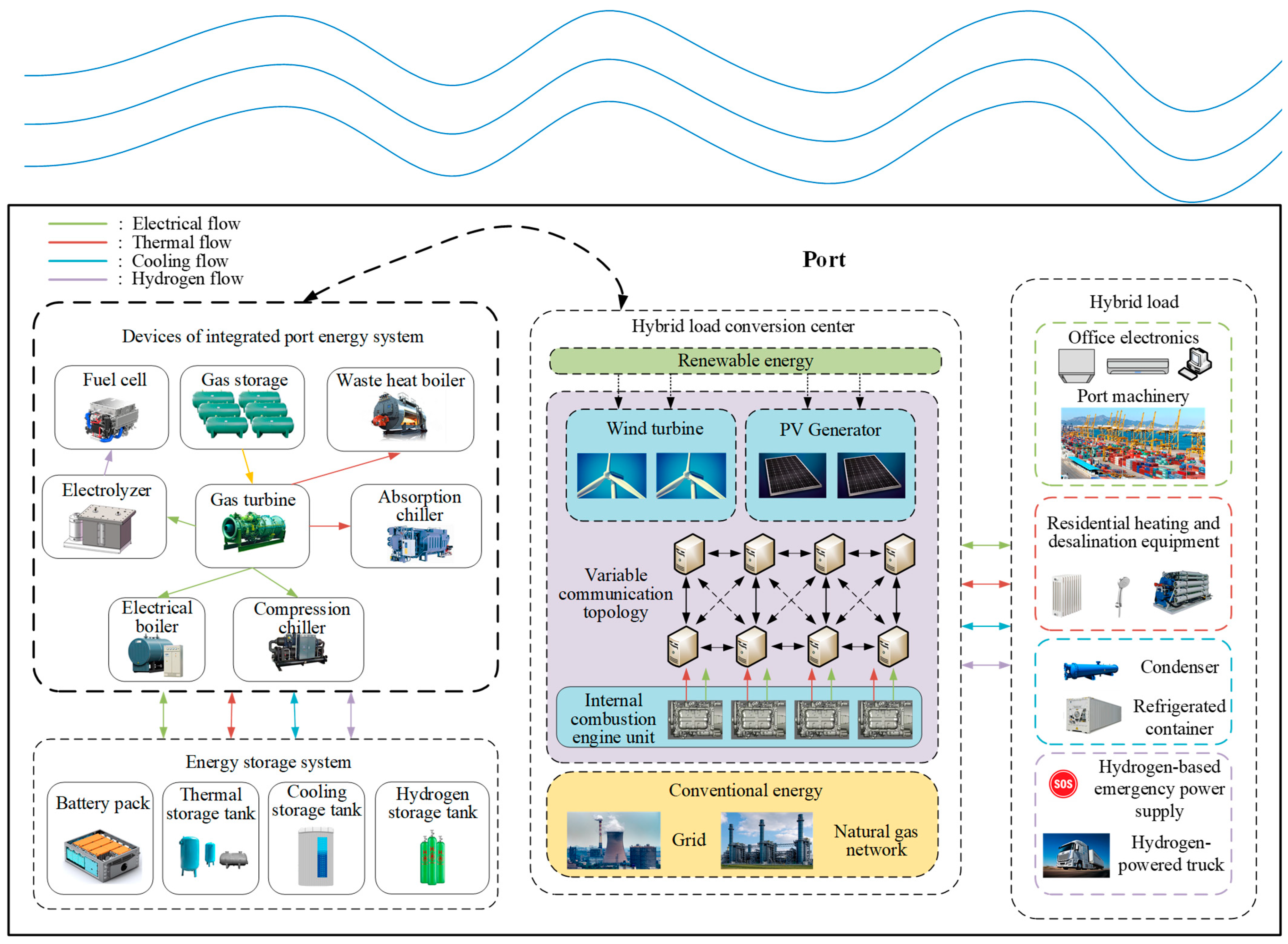
3.1. The Structure of the IPES

In the transmission processes of electricity, thermal, cooling, and hydrogen, the integrated port energy system (IPES) couples electrical energy, thermal energy, and cooling energy through combined cooling heating and power (CCHP) units. It connects renewable energy, hydrogen, and electricity through devices such as electrolyzers and fuel cells [25]. Thermal energy deficiencies are supplemented by electric boilers, while cooling energy deficits are addressed by compression chiller units. In the case of an imbalance between the energy supply and demand sides, surplus or insufficient energy can be stored or supplemented through the energy storage system (ESS) to achieve higher operational efficiency [26]. As discussed above, the structure of the IPES is illustrated in Figure 3.

As shown in Figure 3, the IPES is a hybrid energy system comprising a renewable energy system (RES), integrating CCHP, as well as the electrical/thermal/cooling/hydrogen ESS. The IPES can fully exploit the substitution effect of low-grade energy sources such as cooling and heating for high-grade electrical energy, enabling cascaded utilization of energy to enhance overall energy efficiency. Through the efficient utilization of the horizontal links within the system, encompassing electrical, gas, cooling, and thermal processes, and vertically coordinating multiple energy flows, the IPES effectively mitigates fluctuations caused by renewable energy, thereby increasing the penetration rate of renewable energy and improving energy quality while reducing energy costs [27]. As a result, the development of IPESs plays a positive role in enhancing energy efficiency, reducing environmental pollution, strengthening energy security, and optimizing energy structures.

3.2. The Equipment Model of the IPES

3.2.1. Energy Production Equipment

(1)

Wind turbine (WT)

The output of wind power generation systems is closely related to the weather conditions. The variability of weather leads to different wind speeds in different years, seasons, and even at different times within the same day. In this section, the widely used two-parameter Weibull distribution is employed to fit the probability distribution of actual wind speeds. The probability density function of the Weibull distribution can be formulized as follows [28]:

$$f\left(V\right)=\left({\displaystyle \frac{k}{c}}\right){\left({\displaystyle \frac{V}{c}}\right)}^{k-1}exp\left[-{\left({\displaystyle \frac{V}{c}}\right)}^k\right]$$

(7)

where V denotes the wind speed at the hub of the WT (m/s); c and k are the scale and shape parameters, respectively. These parameters can be obtained through statistical analysis of wind speed historical data. The equations for c and k can be formulized as

$$k={\left({\displaystyle \frac{{\delta }_v}{{\mu }_v}}\right)}^{-1.068}$$

(8)

$$c={\displaystyle \frac{{\mu }_v}{\Gamma \left(1+1/k\right)}}$$

(9)

where Γ denotes the gamma function; μ_v and δ_v denote the mean and standard deviation of historical wind speed data, respectively.

(2)

Photovoltaic (PV) cells

As an unstable power source, PV cells are susceptible to environmental conditions that can impact their output. The widely employed silicon solar cell analytical model can be formulized by Equation (10) [29]:

$$\left\{\begin{array}{l}I=I_{SC}\left\{1-C_1\left[exp\left(\frac{V}{C_2{V}_{OC}}\right)-1\right]\right\}\\ C_1=\left(1-{\displaystyle \frac{I_{mref}\cdot S/S_{ref}\cdot \left(1+\alpha \Delta T\right)}{I_{SCref}\cdot S/S_{ref}\cdot \left(1+\alpha \Delta T\right)}}\right)\exp \left(-{\displaystyle \frac{V_{mref}ln\left(e+b\Delta S\right)\left(1-c\Delta T\right)}{C_2\cdot V_{OCref}ln\left(e+b\Delta S\right)\left(1-c\Delta T\right)}}\right)\\ C_2=\left({\displaystyle \frac{V_{mref}ln\left(e+b\Delta S\right)\left(1-c\Delta T\right)}{V_{OCref}ln\left(e+b\Delta S\right)\left(1-c\Delta T\right)}}-1\right){\left[ln\left(1-{\displaystyle \frac{I_{mref}\cdot S/S_{ref}\cdot \left(1+\alpha \Delta T\right)}{I_{SCref}\cdot S/S_{ref}\cdot \left(1+\alpha \Delta T\right)}}\right)\right]}^{-1}\end{array}\right.$$

(10)

where S_ref = 1000 W/m² and T_ref = 25 °C are the reference irradiation and temperature, respectively; ∆S = S − S_ref is the difference between the current irradiation S and its reference S_ref; ∆T = T − T_ref is the difference between the current temperature T and its reference T_ref; I_SCref, V_OCref, I_mref, and V_mref are the parameters of the PV panel, which can be provided by its producer; a, b, and c are equal to 0.0025 (/°C), 0.0005 (W/m²) and 0.00288 (/°C), respectively; e denotes the base of the natural logarithm, which is equal to 2.71828.

3.2.2. Energy Conversion Equipment

(1)

Gas turbine (GT)

As one of the core components of CCHP systems, GTs play a crucial role in influencing the overall performance of CCHP systems. The GT generates electricity using natural gas as a feedstock, and the exhaust gases produced can be reclaimed for additional heating and cooling purposes. The mathematical model of GT can be formulized as shown in Equation (11) [30]:

$$\left\{\begin{array}{l}{P}_{GT}^E\left(t\right)={\alpha }_{GT}^E\cdot V_{GT}\left(t\right)H_{Gas}\\ P_{GT}^H\left(t\right)=(1-{\alpha }_{GT}^H-{\alpha }_{GT}^{loss})\cdot V_{GT}\left(t\right)H_{Gas}\end{array}\right.$$

(11)

where V_GT (t) denotes the quantity of natural gas input to the gas turbine (m³); H_Gas is the heating value of natural gas, with a specified value of 9.78 (MWh)/m³; $P_{GT}^E\left(t\right)$ is the electrical power output of the GT (MW); $P_{GT}^H\left(t\right)$ is the utilizable heat value of the discharged flue gas (MW); ${\alpha }_{GT}^E$ and ${\alpha }_{GT}^H$ denote the power generation efficiency and heat recovery efficiency of the GT, respectively; ${\alpha }_{GT}^{loss}$ denotes the heat dissipation loss coefficient.

(2)

Waste heat boiler/Absorption chiller (WHB/AC)

Regarding the waste heat generated during the power generation of the GT unit as mentioned above, it is possible to utilize a complementary WHB/AC to recover the waste heat, thereby producing cooling or heating. The heating and cooling capacity of the waste heat absorption chillers and heating unit is linearly related to the utilizable waste heat. It can be specifically formulized as shown in Equations (12)–(14) [31,32]:

$$\left\{\begin{array}{l}{P}_{WHB}^H\left(t\right)={\eta }_{WHB}^H{P}_{Re}\left(t\right)\\ P_{WHB}^{H\_min}\le P_{WHB}^H\left(t\right)\le P_{WHB}^{H\_max}\end{array}\right.$$

(12)

$$\left\{\begin{array}{l}{P}_{AC}^C\left(t\right)={\eta }_{AC}^C{P}_{Re}\left(t\right)\\ P_{AC}^{C\_min}\le P_{AC}^C\left(t\right)\le P_{AC}^{C\_max}\end{array}\right.$$

(13)

$${\displaystyle \frac{P_{WHB}^H\left(t\right)}{{\eta }_{WHB}^H}}+{\displaystyle \frac{P_{AC}^C\left(t\right)}{{\eta }_{AC}^C}}=P_{Re}\left(t\right)$$

(14)

where P_Re (t) denotes the recoverable waste heat (MW); $P_{AC}^C\left(t\right)$ and $P_{WHB}^H\left(t\right)$ denote the cooling and heating power (MW); ${\eta }_{AC}^C$ and ${\eta }_{WHB}^H$ denote the efficiency of cooling and heating, with specified values of 1.2 and 0.9 in this study; $P_{AC}^{C\_min}$, $P_{WHB}^{H\_min}$, $P_{AC}^{C\_max}$ and $P_{WHB}^{H\_max}$ denote the minimum and maximum cooling/heating power (MW), respectively.

(3)

Electric boiler (EB)

When a CCHP system with a certain capacity is unable to meet the heat demand, it is necessary to use an EB for heating. The specific calculation is shown in Equation (15) [33]:

$$\left\{\begin{array}{l}{P}_{EB}^H\left(t\right)={\eta }_{EB}{P}_{EB}^E\left(t\right)\\ P_{EB}^{H\_min}\le P_{EB}^H\left(t\right)\le P_{EB}^{H\_max}\end{array}\right.$$

(15)

where $P_{EB}^H\left(t\right)$ and $P_{EB}^E\left(t\right)$ denote the heating power and electrical power of the electric heating equipment during t-th time period, respectively; η_EB is the conversion coefficient of EB; $P_{EB}^{H\_min}$ and $P_{EB}^{H\_max}$ denote the minimum and maximum heating power, respectively.

(4)

Compression chiller (CC)

Similarly, when a CCHP system with a certain capacity is unable to meet the cold demand, it is necessary to use a CC system for cooling. The output of CC can be formulized as shown in Equation (16) [34]:

$$\left\{\begin{array}{l}{P}_{CC}^C\left(t\right)={\eta }_{CC}{P}_{CC}^E\left(t\right)\\ P_{CC}^{C\_min}\le P_{CC}^C\left(t\right)\le P_{CC}^{C\_max}\end{array}\right.$$

(16)

where η_CC denotes the coefficient of the CC; $P_{CC}^E\left(t\right)$ is the electrical power consumption of the CC (MW); $P_{CC}^C\left(t\right)$ is the refrigeration power of the CC; $P_{CC}^{C\_min}\left(t\right)$ and $P_{CC}^{C\_max}\left(t\right)$ denote the minimum and maximum power of the CC, respectively.

(5)

Electrolyzer (EL)

The electrolysis of water to produce hydrogen is the most widely used method in industrial hydrogen production, and the EL is the core device in the progress of water electrolysis. In IPESs, the surplus renewable energy can be utilized to generate hydrogen through ELs. The output of the EL can be formulized as shown in Equation (17) [35]:

$$\left\{\begin{array}{l}{P}_{EL}^{H_2}\left(t\right)={\displaystyle \frac{{\eta }_{EL}{P}_{EL}^E\left(t\right)}{L_{H_2}}}\\ P_{EL}^{H_2\_min}\le P_{EL}^{H_2}\left(t\right)\le P_{EL}^{H_2\_max}\end{array}\right.$$

(17)

where η_EL and $P_{EL}^E\left(t\right)$ denote the electricity generation efficiency and input electrical power of EL, respectively; $L_{H_2}$ is the lower heating value of hydrogen, which is set to 39.4 kWh/kg in this study; $P_{EL}^{H_2\_min}$ and $P_{EL}^{H_2\_max}$ denote the minimum and maximum power of the EL output.

(6)

Fuel cell (FC)

The output of the hydrogen FC can be formulized as shown in Equation (18) [36]:

$$\left\{\begin{array}{l}{P}_{FC}^E\left(t\right)={\eta }_{FC}{P}_{FC}^{H_2}\left(t\right)\\ P_{FC}^{E\_min}\le P_{FC}^E\left(t\right)\le P_{FC}^{E\_max}\end{array}\right.$$

(18)

where $P_{FC}^{H_2}\left(t\right)$ denotes the input power of the hydrogen FC at the t-th time period, $P_{FC}^E\left(t\right)$ denotes the electrical output power of the hydrogen FC at the t-th time period, and η_FC denotes the electrical efficiency of the hydrogen FC; $P_{FC}^{E\_min}$ and $P_{FC}^{E\_max}$ denote the minimum and maximum power of the FC, respectively.

3.2.3. Energy Storage Devices (ESDs)

ESDs can enhance system reliability and flexibility. The energy storage options available for port facilities include lithium batteries (LIBs), thermal storage devices (TSDs), cooling storage devices (CSDs), and hydrogen storage devices (HSDs). The specific model formulas are given in [37,38].

The energy changes before and after the charging/discharging can be formulized as shown in Equation (19):

$$E_x\left(t\right)=E_x\left(t-1\right)\left(1-{\epsilon }_x\right)+\left[P_x^{ch}\left(t\right){\alpha }_x-{\displaystyle \frac{P_x^{dis}\left(t\right)}{{\beta }_x}}\right]\Delta t,x\in J^S$$

(19)

where E_x (t − 1) and E_x (t) are the state of charge of the ESD before and after charging/discharging, respectively; ε_x is the energy self-discharge rate; $P_x^{ch}\left(t\right)$ and $P_x^{dis}\left(t\right)$ are the charging and discharging power, respectively; α_x and β_x denote the charging and discharging efficiencies, respectively; J^S denotes the ESS set, including LIBs, TSDs, CSDs, and HSDs.

In addition, the ESS must meet the following constraints:

(1)

The capacity constraints of the ESD can be represented by Equation (20):

$$E_x^{min}\le E_x\left(t\right)\le E_x^{max}$$

(20)

where $E_x^{min}$ and $E_x^{max}$ denote the minimum and maximum capacity of the ESD.

(2)

The maximum charging/discharging power constraints can be formulized as shown in Equation (21):

$$\left\{\begin{array}{l}0\le P_x^{ch}\left(t\right)\le {\delta }_x^{ch}\left(t\right)\cdot P_x^{ch\_max}\\ 0\le P_x^{dis}\left(t\right)\le {\delta }_x^{dis}\left(t\right)\cdot P_x^{dis\_max}\end{array}\right.$$

(21)

where $P_x^{ch}\left(t\right)$ and ${\delta }_x^{dis}\left(t\right)$ are binary variables, taking values between 0 and 1; $P_x^{ch\_max}$ and $P_x^{dis\_max}$ denote the maximum charging/discharging power, respectively.

(3)

The constraint of prohibiting charging and discharging simultaneously can be described as shown in Equation (22):

$${\delta }_x^{ch}\left(t\right)+{\delta }_x^{dis}\left(t\right)\le 1$$

(22)

(4)

The SOC terminal state constraint is shown in Equation (23):

$$E_x\left(0\right)=E_x\left(T\right)$$

(23)

Specifically, the end state of the dispatching period E_x(T) should be equal to the initial state E_x(0).

3.3. The Dispatching Model of the IPES

The dispatching model of the IPES comprises an objective function and constraint functions. The objective function minimizes the combined costs of energy consumption and carbon emissions, while the constraint functions maintain an overall energy source balance and restrict energy exchange with the grid within specified limits.

3.3.1. The Objective Function

In IPESs, the costs mainly come from energy consumption costs, equipment maintenance costs, and carbon emission costs. Among these, the energy consumption costs include the costs of purchasing electricity, purchasing gas, and purchasing hydrogen.

Specifically, the operating costs of the entire system include the cost of electricity exchanged with grid C_Grid(t), fuel costs (i.e., C_Gas(t)), maintenance costs (i.e., C_Fix(t)), hydrogen energy costs (i.e., C_Hyd(t)) and the carbon emission costs (i.e., C_Emi(t)). The objective function can be formulized as shown in Equation (24):

$$minC\left(t\right)=C_{Grid}\left(t\right)+C_{Gas}\left(t\right)+C_{Fix}\left(t\right)+C_{Hyd}\left(t\right)+C_{Emi}\left(t\right)$$

(24)

The specific expression for each energy cost is illustrated as follows.

(1)

Electricity grid exchange cost

$$C_{Grid}\left(t\right)={\displaystyle \frac{C_{pur}\left(t\right)+C_{se}\left(t\right)}{2}}{P}_{Grid}\left(t\right)+{\displaystyle \frac{C_{pur}\left(t\right)-C_{se}\left(t\right)}{2}}\left|P_{Grid}\left(t\right)\right|$$

(25)

where C_pur(t) and C_se(t) denote the prices of purchasing and selling electricity, respectively; P_Grid(t) denotes the quantity of power exchanged with the grid. Note that P_Grid(t) > 0 indicates that the IPES purchased power from the grid, and P_Grid(t) < 0 indicates the opposite. The term “(C_pur(t) + C_se(t)) × P_Grid(t)/2” calculates the average cost or benefit of the electricity transaction, where C_pur(t) is the price of purchasing electricity and C_se(t) is the price of selling electricity. This part of the cost or benefit aligns with the direction of the power flow. The term “(C_pur(t) − C_se(t)) × P_Grid(t)/2” calculates the additional cost or benefit due to the difference between the purchase and sale prices of electricity. The absolute value |P_Grid(t)| ensures that this part of the cost or benefit is always positive, as it is proportional to the amount of power flow and independent of the direction.

(2)

Fuel cost

$$C_{Gas}\left(t\right)=C_{Gas}\cdot {\displaystyle \frac{P_{GT}\left(t\right)}{{\eta }_{GT}}}$$

(26)

where P_GT(t) is the GT load power, η_GT is the efficiency of GT, and C_Gas is the gas price.

(3)

The maintenance cost of the equipment

$$C_{Fix}\left(t\right)={\displaystyle {\sum }_1^j{P}_j\left(t\right)\cdot C_j^{Fix}},j\in J^R$$

(27)

where P_j(t) is the electrical load of the IPES; C_j Fix is the unit electricity price for the IPES; J^R denotes the collection of dispatching equipment, including GT, CCHP, CC, etc.

(4)

The cost of purchasing hydrogen energy

$$\left\{\begin{array}{l}{C}_{Hyd}\left(t\right)=P_{ex}^{H_2}\left(t\right)\cdot C_{H_2}\left(t\right)\\ P_{ex}^{H_2}\left(t\right)=\left(P_{Load}^{H_2}\left(t\right)-P_{EL}^{H_2}\left(t\right)\right)\end{array}\right.$$

(28)

where $P_{EL}^{H_2}\left(t\right)$ denotes the hydrogen energy from the electrolyzers; $P_{Load}^{H_2}\left(t\right)$ is the hydrogen load of the port; $P_{ex}^{H_2}\left(t\right)$ denotes the equal power of hydrogen energy exchanged with the energy web; $C_{H_2}\left(t\right)$ denotes the purchasing/selling price of hydrogen energy. Note that if $P_{ex}^{H_2}\left(t\right)<0$, $C_{H_2}\left(t\right)$ is the selling price. On the contrary, $C_{H_2}\left(t\right)$ is the purchasing price.

(5)

The cost of carbon emission

The carbon emissions primarily consist of carbon emissions released when using electricity, natural gas, thermal, and cooling energy, as shown in Equation (29):

$$C_{Emi}(t)=C_{Emi}^E(t)+C_{Emi}^G(t)+C_{Emi}^H(t)+C_{Emi}^C(t)$$

(29)

where C_Emi(t) denotes the total carbon emission cost; $C_{Emi}^E(t)$ denotes the carbon emission cost of electricity; $C_{Emi}^G(t)$ denotes the carbon emission cost of natural gas; $C_{Emi}^H(t)$ denotes the carbon emission cost of thermal energy; $C_{Emi}^C(t)$ denotes the carbon emission cost of cooling energy.

The carbon emissions from electricity and natural gas are composed of two parts: the equivalent emissions from purchasing electricity from the grid and purchasing gas from the gas network, as shown in Equation (30) [39]

$$\left\{\begin{array}{l}{C}_{Emi}^E\left(t\right)=\epsilon \cdot {\beta }_E\cdot P_{G\mathrm{rid}}\left(t\right)\\ C_{Emi}^G\left(t\right)=\epsilon \cdot {\beta }_G\cdot {\displaystyle \frac{P_{GT}\left(t\right)}{{\eta }_{GT}}}\end{array}\right.$$

(30)

where ε denotes the unit carbon emission treatment cost; β_E and β_G denote the equivalent carbon emission coefficient for purchasing electricity and gas, and are set to 0.972 kg/kWh and 0.230 kg/kWh, respectively [40].

Since the carbon emissions from thermal and cooling energy cannot be directly calculated, conversion factors are used to change them into carbon emissions from electricity and natural gas for accounting purposes, as shown in Equation (31):

$$\left\{\begin{array}{l}{C}_{Emi}^H\left(t\right)={\beta }_E\cdot {\lambda }_E\cdot P_H\left(t\right)+{\beta }_G\cdot {\lambda }_G\cdot P_H\left(t\right)\\ C_{Emi}^C\left(t\right)={\beta }_E\cdot {\lambda }_E\cdot P_C\left(t\right)+{\beta }_G\cdot {\lambda }_G\cdot P_C\left(t\right)\end{array}\right.$$

(31)

where λ_E denotes the conversion factor from thermal energy to electricity and from cooling energy to electricity, taken as 0.6 in this paper; λ_G denotes the conversion factor from thermal energy to natural gas and from cooling energy to natural gas, taken as 0.4 in this paper; P_H(t) and P_C(t) denote the purchased thermal energy and cooling energy, respectively.

3.3.2. The Constraint Function

The constraint conditions include the energy balance constraints and the power exchange constraints. Specifically, the energy balance constraint ensures that the total energy input to the system is equal to the total energy output from the system. The power exchange constraints ensure that the power exchange between the system and the energy network remains within the daily limits. Otherwise, there may be situations where the system ceases power exchange with the energy network during specific periods (such as peak energy price periods) or engages in excessive trading during other periods (such as off-peak energy price periods).

The constraint functions in the developed model can be formulized as shown in the following equations:

(1)

The electricity energy balance constraint

$$\begin{array}{l}{P}_{GT}^E\left(t\right)+P_{FC}^E\left(t\right)+P_{ex}^E\left(t\right)+P_{WT}^E\left(t\right)+P_{PV}^E\left(t\right)+P_{Bdis}^E\left(t\right)\\ =P_{Load\_dr}^E\left(t\right)+P_{EL}^E\left(t\right)+P_{EC}^E\left(t\right)+P_{Bch}^E\left(t\right)+P_{EB}^E\left(t\right)\end{array}$$

(32)

where $P_{Load\_dr}^E\left(t\right)$ denotes the electrical load after the demand response, which consists of electrical load $P_{Load}^E\left(t\right)$ and demand response load $P_{DR}^E\left(t\right)$. It can be formulized as shown in Equation (33).

$$P_{Load\_dr}^E(t)=P_{Load}^E(t)+P_{DR}(t)$$

(33)

where P_DR(t) is composed of transferred load, cut load, and interrupted load. It can be formulized as shown in Equation (34).

$$P_{DR}\left(t\right)=P_{in}\left(t\right)-P_{out}\left(t\right)-P_{cut}\left(t\right)-P_{\mathrm{int}}\left(t\right)$$

(34)

where $P_{Trans\_in}^E\left(t\right)$ denotes the load transferred into the port, $P_{Trans\_out}^E\left(t\right)$ denotes the load transferred out of the port, $P_{Cut}^E\left(t\right)$ denotes the cut load, and $P_{Interr}^E\left(t\right)$ denotes the interrupted load.

(2)

The thermal energy balance constraint

$$P_{WHB}^H\left(t\right)+P_{EB}^H\left(t\right)+P_{HSdis}^H\left(t\right)=P_{Load}^H\left(t\right)+P_{HSch}^H\left(t\right)$$

(35)

(3)

The cold energy balance constraint

$$P_{AC}^C\left(t\right)+P_{CC}^C\left(t\right)+P_{CSdis}^C\left(t\right)=P_{Load}^C\left(t\right)+P_{CSch}^C\left(t\right)$$

(36)

(4)

The hydrogen energy balance constraint

$$P_{EL}^{H_2}\left(t\right)+P_{H_{2}Sdis}^{H_2}\left(t\right)=P_{Load}^{H_2}\left(t\right)+P_{FC}^{H_2}\left(t\right)+P_{H_{2}Sch}^{H_2}\left(t\right)$$

(37)

(5)

The power exchange constraint with the grid

$$P_{G\mathrm{rid}}^{min} \le P_{G\mathrm{rid}}\left(t\right)\le P_{G\mathrm{rid}}^{max}$$

(38)

where $P_{G\mathrm{rid}}^{min}$ and $P_{G\mathrm{rid}}^{max}$ denote the lower and upper bounds of $P_{G\mathrm{rid}}\left(t\right)$.

4. Experimental Results and Analysis

In this section, the efficiency of the developed dispatching method is comprehensively verified by case studies, and the impact of storage capacity on dispatching performance is also discussed in detail.

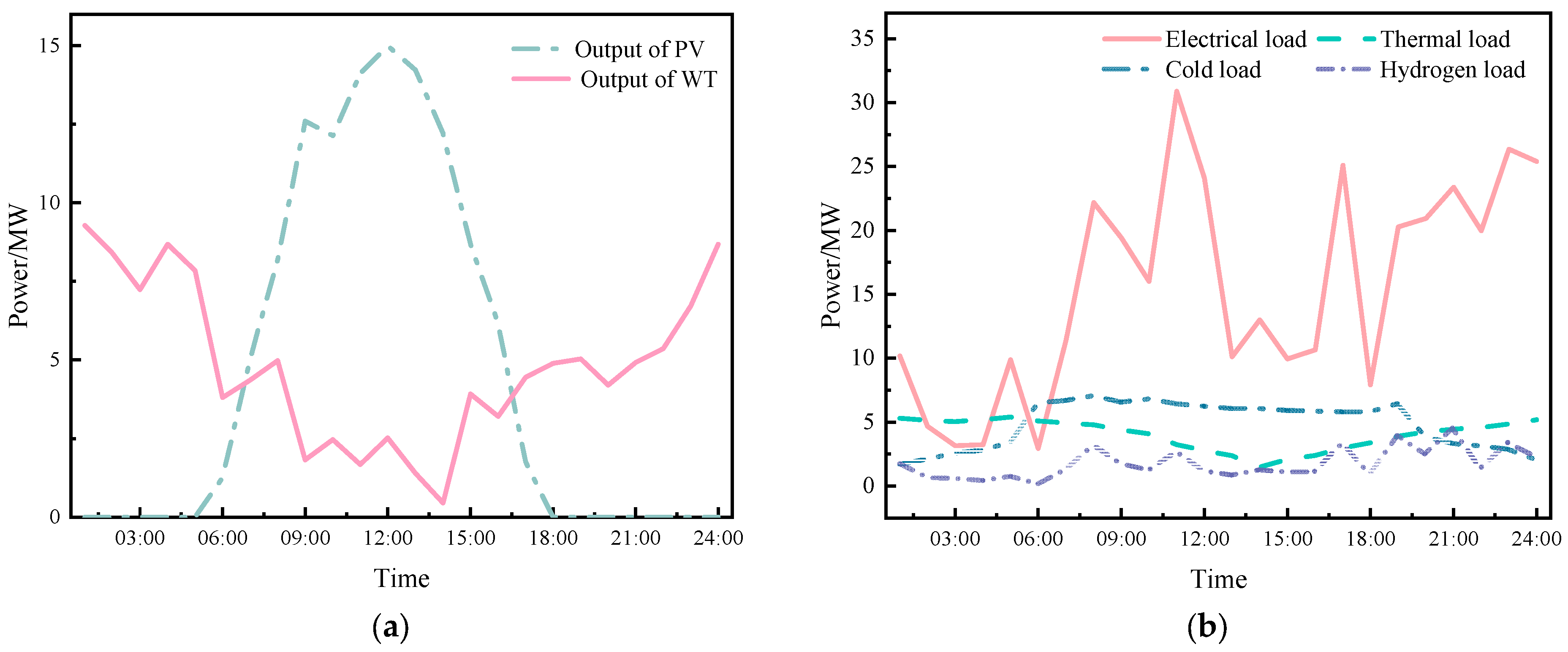
4.1. Parameter Settings

In this section, the daily electricity/thermal/cooling/hydrogen loads and the renewable energy output are plotted in Figure 4.

In addition, the detailed construction parameters of all energy equipment and ESDs in the IPES are listed in

Table 3. Construction parameters of the dispatching equipment and ESDs.

Name	Input Energy	Output Energy	Efficiency	Unit Construction Cost/(RMB/MW)	Useful Life/Year
PV	Renewable	Electricity	0.17	5,000,000	20
WT	Renewable	Electricity	0.39	6,500,000	20
GT	Electricity	Thermal	0.48	1,000,000	20
EB	Electricity	Thermal	0.98	1,200,000	10
EL	Electricity	Hydrogen	0.83	600,000	10
FC	Hydrogen	Electricity	0.65	200,000	1
CC	Electricity	Cooling	3.00	600,000	20
AC	Thermal	Cooling	0.80	600,000	20
WHB	Thermal	Thermal	0.90	960,000	10
LIB	Electricity	Electricity	0.98	780,000	15
TSD	Thermal	Thermal	0.90	90,000	10
CSD	Cooling	Cooling	0.90	90,000	10
HSD	Hydrogen	Hydrogen	0.95	669,000	15

[4,39,41].

In addition to the construction parameters shown in Table 3, the performance of the IPES is also directly influenced by the operating parameters of all equipment or devices. As a result, the detailed operating parameters of the ESDs are listed in

Table 4. Operating parameters of the ESDs.

Name	Capacity/(MWh)	Self-Loss Rate	Initial SOE	Charging/Discharging Efficiency	Maintenance Cost/(RMB/MWh)	Max Charging/Discharging Ramping Rate/(MW/h)
LIB	8	0.01	0.1	0.9/0.95	96	0.6/0.6
TSD	6	0.02	0.12	0.9/0.9	16	0.6/0.6
CSD	6	0.02	0.25	0.9/0.9	16	0.6/0.6
HSD	3	--	0.13	0.9/0.9	18	0.6/0.6

[41,42,43].

The operating parameters of the dispatching equipment exhibit slight differences from the ESDs. The detailed operating parameters for the dispatching equipment are listed in

Table 5. Operating parameters of the dispatching equipment.

Name	Capacity/(MWh)	Ramping Rate/(MW/h)	Maintenance Cost/(RMB/MWh)
PV	18	--	23.5
WT	20	--	19.6
GT	8	−1.0/1.0	25
EB	6	−1.0/1.0	16
EL	5	−1.0/1.0	24
FC	5	−1.0/1.0	26
CC	6	−1.0/1.0	20
AC	6	−1.0/1.0	20
WHB	6	−1.0/1.0	17

[41,43,44].

Moreover, the time-of-use price for different kinds of energies are employed in the following experiments, which are listed in

Table 6. Time-of-use prices of energies.

Time	Purchasing Electricity/(RMB/MWh)	Selling Electricity/(RMB/MWh)	Purchasing Gas/(RMB/MWh)	Purchasing Hydrogen Energy/(RMB/MWh)	Selling Hydrogen Energy/(RMB/MWh)
Off-peak period	300	250	320	498	340
Standard period	780	680	320	498	340
Peak period	1200	900	320	498	340

[4].

It is worth noting that the off-peak periods consist of 1:00–7:00 and 23:00–24:00, the standard periods are 8:00–11:00 and 15:00–18:00, and the peak periods consist of 12:00–14:00 as well as 19:00–22:00.

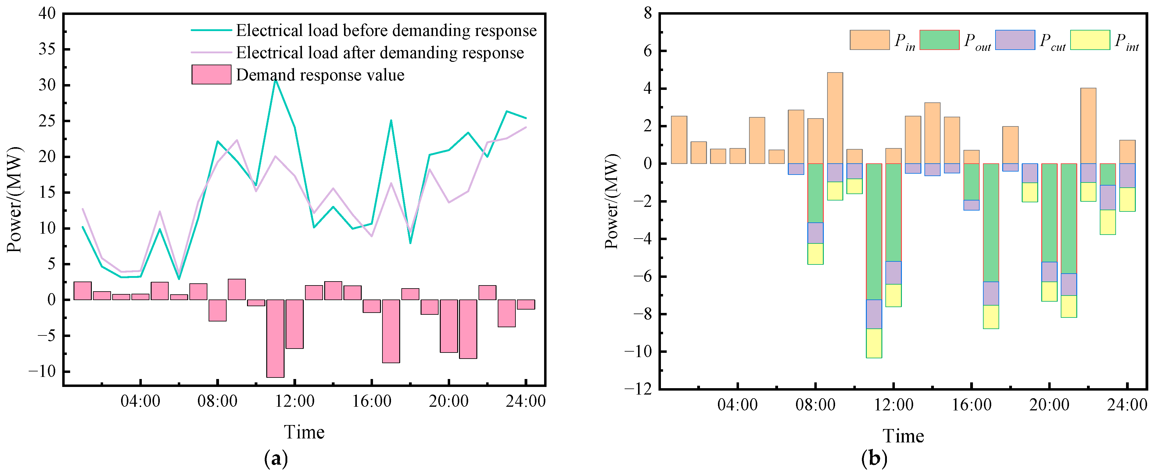
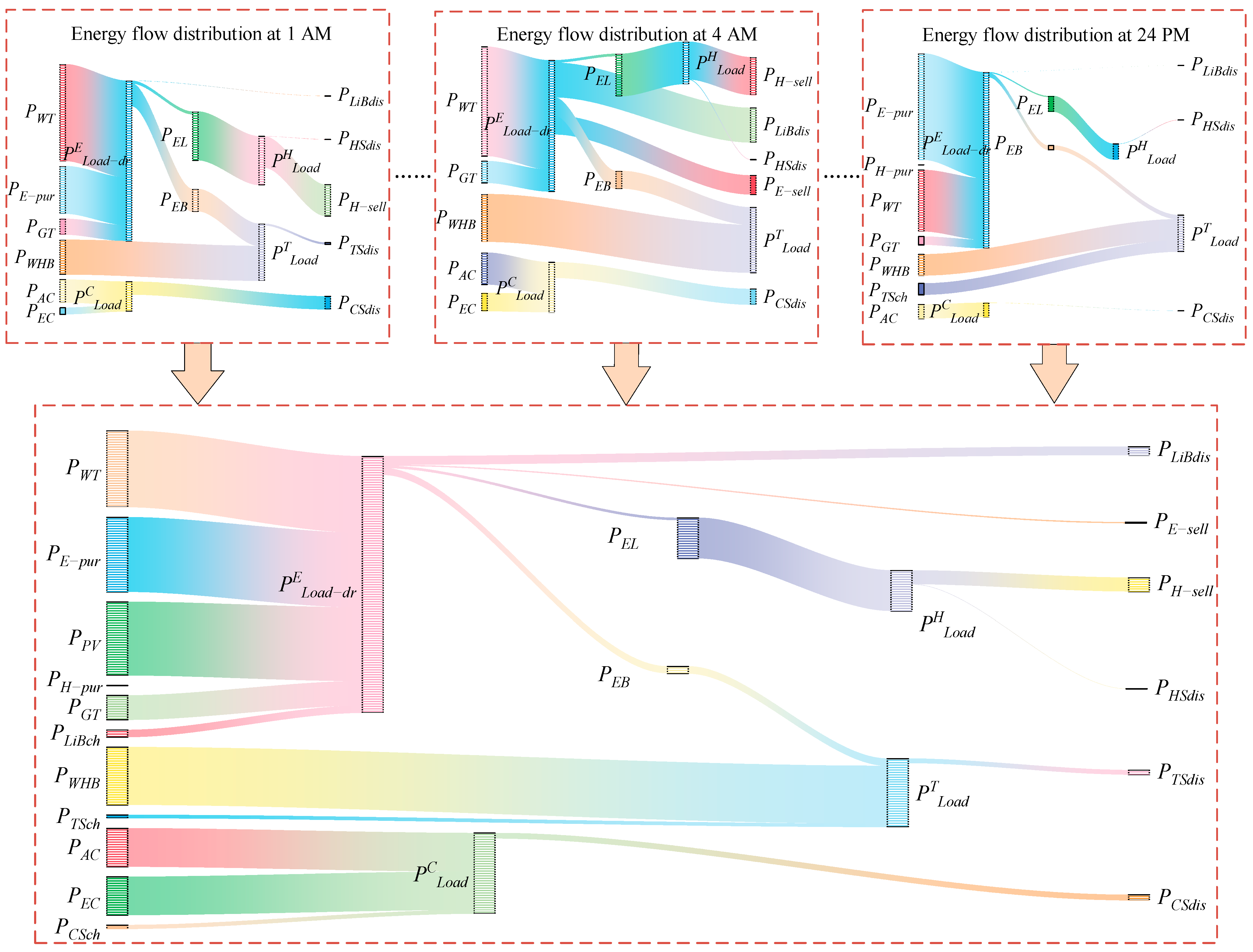
4.2. Experimental Results and Analysis

The model developed in this study is a mixed-integer linear programming model, which can be solved by the CPLEX commercial solver. The demand response results are as follows.

As shown in Figure 5a, there is a significant change in the port’s electricity load compared to before the demand response. Specifically, the peak-to-valley difference in the port’s electricity load has decreased after load shifting. In addition, the total electricity load of the port has decreased compared to before the response, after load reduction and interruption.

As shown in Figure 5b, for transferable loads, the port effectively disperses the peak load to other scheduling periods, achieving a significant “peak shaving and valley filling” effect. And the port has effectively reduced the reducible load in most scheduling periods, mainly reflected in office and living electricity usage. For interruptible loads such as refrigerated container electricity, the port mainly participates in demand response through intermittent power outages. Moreover, the port’s energy cost has been reduced from the original RMB 368,750 to RMB 136,830.

The visualization graphs for the daily dispatching results of electricity, thermal, cooling, and hydrogen loads are shown in Figure 6.

As shown in Figure 6a, the outputs of WTs and PV cells have the highest priority for supplying electricity power, as the utilization of these types of renewable energy is free. Then, additional electricity is purchased from the grid or generated by the FCs, GTs, and LIBs if the output of the RES is inefficient. On the contrary, if the outputs of WTs and PV cells are adequate, some of the surplus power is stored in LIBs, and some is used to produce hydrogen by ELs. Finally, the remaining portion can be used by EBs or CCs. From 1:30 a.m. to 4:30 a.m., the load demand is the lowest. Then, from 12:30 p.m. to 4:00 p.m., the renewable energy brings the maximum electricity revenue to the system. Therefore, during these two periods, the net electricity load is negative, indicating that this portion of electricity can be sold back to the grid.

As depicted in Figure 6b, the port’s thermal energy is primarily supplied in two forms: one is supplied through the utilization of residual heat from GTs, and the other is supplied by the EBs. Specifically, the high-temperature flue gas generated by GTs is first recovered and utilized to produce low-quality thermal energy via the waste heat boiler, in order to maximize the utilization of GTs. If the thermal energy produced by the waste heat boiler is insufficient to meet the thermal load requirements, the EBs consume electricity to generate thermal energy. In addition, the surplus thermal energy generated during the heating process is stored in the TSD and supplied to the thermal load when the thermal energy price is high, thereby reducing heating costs.

As indicated in Figure 6c, the method of supplying the port’s cooling energy is similar to that for thermal energy, primarily through two forms, HRC and CC. Specifically, the high-temperature flue gas generated by GTs is first directed into the HRC for cooling, maximizing the utilization of GTs. If the HRC cannot meet the cooling load requirements, the CCs consume electricity to generate cooling energy. In addition, the CSD is used to regulate peaks, in order to ensure system stability while reducing energy costs.

As illustrated in Figure 6d, the hydrogen energy in ports is primarily supplied through ELs, which produce hydrogen by water electrolysis. Due to the small hydrogen demand, the electricity needed for ELs can be directly provided by renewable energy sources. The hydrogen energy produced by ELs not only meets the hydrogen demand but also provides excess hydrogen to FCs for power generation, supplying electricity to the system’s electrical load. Similarly, hydrogen energy is supplied with increased flexibility and reduced cost through HSDs.

In summary, the distribution of energy flow in the port on a certain day and its components are shown in Figure 7.

Figure 8 illustrates the variation in the state of energy for four types of ESDs on a certain day. As shown in Figure 4, it can be inferred that the port area has a significant demand for electric power, while its capacity for cold load generation is relatively limited, with a lower output capability. Consequently, there is an increased demand for LIBs and CSDs at the port to mitigate electricity load fluctuations and enhance the mobility of cooling loads. Therefore, in comparison to TSDs and HSDs, the utilization rate of LIBs and CSDs is higher.

4.3. Carbon Emission Analysis

Under different scenarios, the costs and the carbon emissions of the port will vary. This section compares the ESS and IPES by using the scenarios listed in

Table 7. The energy costs of different scenarios.

Scenario	Purchased Electricity Costs (RMB)	Purchased Gas Costs (RMB)	Purchased Thermal Costs (RMB)	Purchased Cooling Costs (RMB)	Purchased Hydrogen Costs (RMB)	Total Costs (RMB)
I (Traditional system)	211,083	—	19,340	19,902	18,473	268,798
II (IPES)	119,851	37,624	—	—	—	5
III (ESS + IPES)	94,293	37,624	—	—	—	131,916

and

Table 8. Daily carbon emissions of different scenarios.

Scenario	Calculate Area	Daily Carbon Emissions/kg
I (Traditional system)	Port area	—
	Power plant area	613,718
	Total	613,718
II (IPES)	Port area	86,051
	Power plant area	290,497
	Total	376,548
III (ESS + IPES)	Port area	62,313
	Power plant area	286,146
	Total	348,459

. The energy costs and carbon emissions for each scenario are calculated, and the results for different scenarios are comprehensively analyzed.

In scenario I, the IPES and ESS are not integrated, and the RES is also not considered. In this context, all the forecasted loads are directly purchased. According to the experimental results listed in Table 8, the purchased electricity cost is RMB 211,083, accounting for approximately 78.53% of the total cost, which is the primary cost of port energy procurement. Due to the absence of an ESS, peak shaving cannot be performed, which directly leads to the coincidence of the peak demand period with the highest energy price period, and the total costs also significantly increase.

In scenario II, an IPES is integrated without an ESS, but the RES is considered. In this context, the cooling, thermal, and hydrogen loads are provided by the energy conversion equipment in the IPES. When considering the energy costs for this part, only the electricity consumed by the energy conversion equipment and the corresponding cost of natural gas need to be considered. Due to the integration of the RES, a portion of electricity is directly supplied by the PV array and WTs. As a result, the purchased electricity costs are significantly reduced to only RMB 119,851.

Although the costs for cooling, thermal, and hydrogen energy procurement are partially added to the electricity purchase costs, the overall reduction compared to scenario I is still 43.22%. Additionally, due to the high weighting of purchased electricity costs, the overall energy costs for the port are reduced by 41.42%, a reduction that aligns closely with the decrease in purchased electricity costs.

In scenario III, the IPES is integrated with an ESS, while the RES is also considered. The ESS allows for a certain displacement between peak demand periods and high-priced energy periods. As a result, the cost of purchased electricity is further reduced to RMB 94,293, a decrease of 55.33% compared to scenario I. Under the same conditions as the IPES, the integration of the ESS results in a 21.33% reduction compared to scenario II. Since the gas price remains constant, the gas purchase cost remains unchanged at RMB 37,624 after integrating the ESS.

While considering energy costs, it is also important to pay attention to the environmental impact of carbon emissions. The carbon emissions calculated using Equation (28) are shown in Table 8. Similarly, an analysis is conducted for the three scenarios mentioned above. Note that the carbon emissions accounted for in this study include the direct carbon emissions from the port area and the carbon emissions generated in the power plant area due to electricity purchasing behavior. And the total carbon emissions under each scenario should be the sum of them.

In scenario I, a total of 613,718 kg of carbon emissions was generated. Since the IPES was not integrated, all energy is purchased directly from the grid, and thus all carbon emissions are attributed to the power plants.

In scenario II, the integration of the IPES and clean energy generation significantly reduced carbon emissions. However, since the energy conversion equipment in the IPES consumes electricity and natural gas to produce other forms of energy, the calculation of carbon emissions for this part is set in the port area, resulting in a total of 86,051 kg of carbon emissions, accounting for 22.85% of the total emissions in this scenario. The net exchange of power with the electricity and gas grids is considered as carbon emissions from power plants, resulting in a total of 290,497 kg of carbon emissions. This represents a 52.67% reduction compared to scenario I. Overall, the total carbon emissions are reduced by 38.64% compared to scenario I, showing a significant decrease.

In scenario III, with the addition of the ESS, carbon emissions in the port area decreased by 27.59%, while carbon emissions from power plants decreased by 1.5%. Overall, total emissions decreased by 7.46% compared to scenario II.

As discussed above, the calculated results align with expectations, indicating that the integration of ESS and IPES can reduce carbon emissions in both the port area and the power plant area. This further validates the feasibility of the optimization method.

5. Conclusions

This study proposes a method for forecasting the electricity load of container ports based on ship arrival and departure schedules as well as port handling tasks. By finely modeling the electricity consumption behavior of port machinery, effective prediction of the main electricity loads of ports, including quay cranes, yard cranes, and shore power, is achieved. On this basis, the overall structure of an integrated port energy system (IPES) considering demand response is studied, in which renewable energy systems, energy storage systems (ESSs), dispatching equipment, and different kinds of loads are included. In order to achieve optimal dispatching of the developed IPES, a dispatching model is also established, and the day-ahead optimal dispatching of the IPES can be implemented based on the forecasted load. Experimental results show that the IPES can reduce the total energy cost of the port by about 43.22%, and carbon emissions can also be decreased by 38.64%. Moreover, demand response has resulted in an additional reduction of RMB 231,920 in the port’s energy costs. Furthermore, the ESS can further reduce the energy cost by 21.33% and decrease carbon emissions by 7.46%. Overall, the developed method ensures the operational efficiency of IPES, reduces port energy costs, and decreases carbon emissions.

This study has conducted load forecasting for port electricity consumption based on a refined model of port machinery and equipment. However, due to the unavailability of actual port electricity load data, it is not possible to verify the forecasting results at present. In future research, we will endeavor to obtain real data from ports or construct a scaled-down model of actual port machinery for experimental validation. This will allow us to further calibrate the forecasting model and enhance its accuracy.

Additionally, the dispatching problem of integrated energy systems is generally divided into two categories: day-ahead and intra-day scheduling. This paper primarily focuses on day-ahead dispatching, while neglecting the intra-day correction. In future research, we will further investigate the intra-day dispatching problem to address this gap.

Furthermore, sensitivity analysis of the experiments is also very important. In the subsequent research process, we will further optimize and increase the sensitivity analysis of the experiments.

In future, more efforts will be made to further optimize the detailed connection structures of IPESs. In addition, regional connections between different ports should be taken into account, and the time dimension of dispatching should also be extended.

References

1. Zhang, J.; Song, Y. Mathematical model and algorithm for the reefer mechanic scheduling problem at seaports. Discret. Dyn. Nat. Soc. 2017, 2017, 4730253. [Google Scholar] [CrossRef]
2. Fiadomor, R. Assessment of Alternative Maritime Power (Cold Ironing) and Its Impact on Port Management and Operations. Master’s Thesis, World Maritime University, Malmö, Sweden, 2009. [Google Scholar]
3. Huang, W.; Yu, M.; Li, H.; Tai, N. Energy Management of Integrated Energy System in Large Ports; Springer Nature: Singapore, 2023. [Google Scholar]
4. Zhao, J.; Mi, H.; Cheng, H.; Chen, S. A planning model and method for an integrated port energy system considering shore power load flexibility. J. Shanghai Jiaotong Univ. 2021, 55, 1577. [Google Scholar]
5. Wang, C.; Chen, Q.; Huang, R. Locating dry ports on a network: A case study on Tianjin Port. Marit. Policy Manag. 2018, 45, 71–88. [Google Scholar] [CrossRef]
6. Pu, Y.; Chen, W.; Zhang, R.; Liu, H. Optimal operation strategy of port integrated energy system considering demand response. In Proceedings of the 2020 IEEE 4th Conference on Energy Internet and Energy System Integration (EI2), Wuhan, China, 30 October–1 November 2020; IEEE: Wuhan, China, 2020; pp. 518–523. [Google Scholar]
7. Song, T.; Li, Y.; Zhang, X.-P.; Wu, C.; Li, J.; Guo, Y.; Gu, H. Integrated port energy system considering integrated demand response and energy interconnection. Int. J. Electr. Power Energy Syst. 2020, 117, 105654. [Google Scholar] [CrossRef]
8. Wang, X.; Wang, S.; Zhao, Q.; Wang, S.; Fu, L. A multi-energy load prediction model based on deep multi-task learning and ensemble approach for regional integrated energy systems. Int. J. Electr. Power Energy Syst. 2021, 126, 106583. [Google Scholar]
9. Fan, G.-F.; Han, Y.-Y.; Wang, J.-J.; Jia, H.-L.; Peng, L.-L.; Huang, H.-P.; Hong, W.-C. A new intelligent hybrid forecasting method for power load considering uncertainty. Knowl.-Based Syst. 2023, 280, 111034. [Google Scholar] [CrossRef]
10. Tan, Z.; De, G.; Li, M.; Lin, H.; Yang, S.; Huang, L.; Tan, Q. Combined electricity-heat-cooling-gas load forecasting model for integrated energy system based on multi-task learning and least square support vector machine. J. Clean. Prod. 2020, 248, 119252. [Google Scholar] [CrossRef]
11. Kim, G.; Lee, G.; An, S.; Lee, J. Forecasting future electric power consumption in Busan New Port using a deep learning model. Asian J. Shipp. Logist. 2023, 39, 78–93. [Google Scholar] [CrossRef]
12. Duan, J.; Tian, Q.; Liu, F.; Xia, Y.; Gao, Q. Optimal scheduling strategy with integrated demand response based on stepped incentive mechanism for integrated electricity-gas energy system. Energy 2024, 313, 133689. [Google Scholar] [CrossRef]
13. Zhang, L.; Li, Q.; Fang, Y.; Yang, Y.; Ren, H.; Fan, L.; Tai, N. Optimization scheduling of community integrated energy system considering integrated demand response. J. Build. Eng. 2024, 98, 111230. [Google Scholar] [CrossRef]
14. Wang, Z.; Liu, Z.; Huo, Y. A distributionally robust optimization approach of multi-park integrated energy systems considering shared energy storage and Uncertainty of Demand Response. Electr. Power Syst. Res. 2025, 238, 111116. [Google Scholar] [CrossRef]
15. Iris, Ç.; Lam, J.S.L. Optimal energy management and operations planning in seaports with smart grid while harnessing renewable energy under uncertainty. Omega 2021, 103, 102445. [Google Scholar] [CrossRef]
16. Zhang, Q.; Qi, J.; Zhen, L. Optimization of integrated energy system considering multi-energy collaboration in carbon-free hydrogen port. Transp. Res. Part E Logist. Transp. Rev. 2023, 180, 103351. [Google Scholar] [CrossRef]
17. Iris, Ç.; Lam, J.S.L. A review of energy efficiency in ports: Operational strategies, technologies and energy management systems. Renew. Sustain. Energy Rev. 2019, 112, 170–182. [Google Scholar] [CrossRef]
18. Shen, W.; Zeng, B.; Zeng, M. Multi-timescale rolling optimization dispatch method for integrated energy system with hybrid energy storage system. Energy 2023, 283, 129006. [Google Scholar] [CrossRef]
19. Zhao, N.; Gu, W. Low-carbon planning and optimization of the integrated energy system considering lifetime carbon emissions. J. Build. Eng. 2024, 82, 108178. [Google Scholar] [CrossRef]
20. Bakar, N.N.A.; Guerrero, J.M.; Vasquez, J.C.; Bazmohammadi, N.; Yu, Y.; Abusorrah, A.; Al-Turki, Y.A. A Review of the Conceptualization and Operational Management of Seaport Microgrids on the Shore and Seaside. Energies 2021, 14, 7941. [Google Scholar] [CrossRef]
21. Parise, G.; Parise, L.; Malerba, A.; Pepe, F.M.; Honorati, A.; Chavdarian, P. Comprehensive Peak-Shaving Solutions for Port Cranes. IEEE Trans. Ind. Appl. 2017, 53, 1799–1806. [Google Scholar] [CrossRef]
22. Tang, G.; Qin, M.; Zhao, Z.; Yu, J.; Shen, C. Performance of peak shaving policies for quay cranes at container terminals with double cycling. Simul. Model. Pract. Theory 2020, 104, 102129. [Google Scholar] [CrossRef]
23. Iris, Ç.; Lam, J.S.L. Recoverable robustness in weekly berth and quay crane planning. Transp. Res. Part B Methodol. 2019, 122, 365–389. [Google Scholar] [CrossRef]
24. Liu, X. Distributionally robust optimization scheduling of port energy system considering hydrogen production and ammonia synthesis. Heliyon 2024, 10, e27615. [Google Scholar] [CrossRef] [PubMed]
25. Nondy, J. 4E analyses of a micro-CCHP system with a polymer exchange membrane fuel cell and an absorption cooling system in summer and winter modes. Int. J. Hydrogen Energy 2024, 52, 886–904. [Google Scholar] [CrossRef]
26. Ouyang, T.; Tan, X.; Tuo, X.; Qin, P.; Mo, C. Performance analysis and multi-objective optimization of a novel CCHP system integrated energy storage in large seagoing vessel. Renew. Energy 2024, 224, 120185. [Google Scholar] [CrossRef]
27. NI, L.; Liu, W.; Wen, F.; Xue, Y.; Dong, Z.; Zheng, Y.; Zhang, R. Optimal operation of electricity, natural gas and heat systems considering integrated demand responses and diversified storage devices. J. Mod. Power Syst. Clean Energy 2018, 6, 423–437. [Google Scholar] [CrossRef]
28. Sunderland, K.; Woolmington, T.; Blackledge, J.; Conlon, M. Small wind turbines in turbulent (urban) environments: A consideration of normal and Weibull distributions for power prediction. J. Wind Eng. Ind. Aerodyn. 2013, 121, 70–81. [Google Scholar] [CrossRef]
29. Tang, R.; Wu, Z.; Li, X. Optimal operation of photovoltaic/battery/diesel/cold-ironing hybrid energy system for maritime application. Energy 2018, 162, 697–714. [Google Scholar] [CrossRef]
30. Shen, X.; Han, Y.; Zhu, S.; Zheng, J.; Li, Q.; Nong, J. Comprehensive power-supply planning for active distribution system considering cooling, heating and power load balance. J. Mod. Power Syst. Clean Energy 2015, 3, 485–493. [Google Scholar]
31. Tavana, M.; Deymi-Dashtebayaz, M.; Gholizadeh, M.; Ghorbani, S.; Dadpour, D. Optimizing building energy efficiency with a combined cooling, heating, and power (CCHP) system driven by boiler waste heat recovery. J. Build. Eng. 2024, 97, 110982. [Google Scholar] [CrossRef]
32. Ibrahim, N.I.; Yahiaoui, A.; Garkuwa, J.A.; Ben Mansour, R.; Rehman, S. Solar cooling with absorption chillers, thermal energy storage, and control strategies: A review. J. Energy Storage 2024, 97, 112762. [Google Scholar] [CrossRef]
33. Zhao, P.; Gou, F.; Xu, W.; Shi, H.; Wang, J. Multi-objective optimization of a hybrid system based on combined heat and compressed air energy storage and electrical boiler for wind power penetration and heat-power decoupling purposes. J. Energy Storage 2023, 58, 106353. [Google Scholar] [CrossRef]
34. Moghaddas-Zadeh, N.; Farzaneh-Gord, M.; Bahnfleth, W.P. Optimal design and operation of the hybrid absorption-compression chiller plants—Energy and economic analysis. J. Build. Eng. 2024, 82, 108182. [Google Scholar] [CrossRef]
35. Bornemann, L.; Lange, J.; Kaltschmitt, M. Optimizing temperature and pressure in PEM electrolyzers: A model-based approach to enhanced efficiency in integrated energy systems. Energy Convers. Manag. 2025, 325, 119338. [Google Scholar] [CrossRef]
36. Amirkhalili, S.A.; Zahedi, A.; Ghaffarinezhad, A.; Kanani, B. Design and evaluation of a hybrid wind/hydrogen/fuel cell energy system for sustainable off-grid power supply. Int. J. Hydrogen Energy 2025, 100, 1456–1482. [Google Scholar] [CrossRef]
37. Villamarín-Jácome, A.; Saltos-Rodríguez, M.; Espín-Sarzosa, D.; Haro, R.; Villamarín, G.; Okoye, M.O. Deploying renewable energy sources and energy storage systems for achieving low-carbon emissions targets in hydro-dominated power systems: A case study of Ecuador. Renew. Energy 2025, 241, 122198. [Google Scholar] [CrossRef]
38. Ju, L.; Lu, X.; Li, F.; Bai, X.; Li, G.; Nie, B.; Tan, Z. Two-stage optimal dispatching model and benefit allocation strategy for hydrogen energy storage system-carbon capture and utilization system-based micro-energy grid. Energy Convers. Manag. 2024, 313, 118618. [Google Scholar] [CrossRef]
39. Patel, D.; Matalon, P.; Oluleye, G. A novel temporal mixed-integer market penetration model for cost-effective uptake of electric boilers in the UK chemical industry. J. Clean. Prod. 2024, 446, 141156. [Google Scholar] [CrossRef]
40. Ma, T.; Wu, J.; Hao, L. Energy flow modeling and optimal operation analysis of the micro energy grid based on energy hub. Energy Convers. Manag. 2017, 133, 292–306. [Google Scholar] [CrossRef]
41. Sadeghian, O.; Shotorbani, A.M.; Mohammadi-Ivatloo, B.; Ghassemzadeh, S. Fuel cell preventive maintenance in an electricity market with Hydrogen storage and Scenario-Based risk management. Sustain. Energy Technol. Assess. 2024, 61, 103587. [Google Scholar] [CrossRef]
42. Jiao, P.; Chen, J.; Cai, X.; Wang, L.; Zhao, Y.; Zhang, X.; Chen, W. Joint active and reactive for allocation of renewable energy and energy storage under uncertain coupling. Appl. Energy 2021, 302, 117582. [Google Scholar] [CrossRef]
43. Dou, X. Comprehensive Energy System Optimization and Operation, Effectiveness Evaluation and Application Research. Master’s Thesis, North China Electric Power University, Beijing, China, 2024. [Google Scholar]
44. Farah, S.; Andresen, G. Investment-based optimisation of energy storage design parameters in a grid-connected hybrid renewable energy system. Appl. Energy 2024, 355, 122384. [Google Scholar] [CrossRef]
Figure 1. Energy conversion diagram.
Jmse 13 00421 g001
Figure 2. Power load curve of the container port on a certain day.
Jmse 13 00421 g002
Figure 3. The structure of the IPES.
Jmse 13 00421 g003
Figure 4. Renewable energy output and the integrated energy loads. (a) Renewable energy output; (b) The integrated energy loads.
Jmse 13 00421 g004
Figure 5. Demand response result graphs. (a) The load curve before and after the demand response; (b) Load regulation.
Jmse 13 00421 g005
Figure 6. Dispatching results of IPES. (a) Electrical dispatching results; (b) Thermal dispatching results; (c) Cooling dispatching results; (d) Hydrogen dispatching results.
Jmse 13 00421 g006
Figure 7. Distribution of energy flow in IPES.
Jmse 13 00421 g007
Figure 8. SOE of ESDs.
Jmse 13 00421 g008