Extraction of Tsunami Signals from Coupled Seismic and Tsunami Waves

Abstract

The generation of an earthquake and a tsunami is a coupled process of radiating seismic waves and exciting tsunamis, and the two types of waves are simultaneously recorded by ocean-bottom pressure sensors. In order to constrain the earthquake source and evaluate the tsunami hazards, it is necessary to separate the tsunami waves. It is traditional to apply a low-pass filter such that the seismic waves are filtered and the tsunami waves remain. However, filtering may also cause distortion of the tsunami waves. In this study, we first use the finite-element method to simulate the generation of seismic and tsunami waves and show that the coupling is a linear superposition of the two waves. We then propose a new method to extract the tsunami waves. First, a low-pass filter with relatively high cutoff frequency that does not affect the tsunami waves is adopted, so that only tsunami waves and low-frequency seismic waves remain. The low-frequency seismic waves satisfy a theoretical equation $p=\rho ha$ (p pressure, $\rho$ water density, h water depth, and a seafloor vertical acceleration), and they can be predicted and removed by utilizing the records of ocean-bottom acceleration. We demonstrate the procedure by numerical simulations and show that the method successfully extracts clean tsunami signals, which is important for earthquake source characterization and tsunami hazard assessment.

1. Introduction

Tsunamis, which are mainly triggered by submarine earthquakes, pose significant risks to coastal communities due to their destructive power and sudden occurrence. The accurate assessment of tsunami threat following an earthquake is essential for hazard mitigation, and timely warnings are important in this manner. After a submarine earthquake occurs, if one can immediately determine whether the earthquake triggers a tsunami and assess the potential severity of the tsunami from the seismic source area, we can take effective measures in time to prevent serious tsunami disasters before the tsunami waves reach the coast. Therefore, it is necessary to record the tsunami waves during the tsunami generation process in the source area. However, tsunami generation is a complex process that radiates coupled seismic and tsunami wave signals in the source region, which are recorded by seafloor pressure gauges and other instruments [1,2,3,4]. Decoupling these signals is critical for separating the tsunami waves, which is also the key to understanding the tsunami’s generation mechanism and potential severity [5].

Theoretical and numerical studies have explored the relationship between seismic and tsunami waves during the tsunami generation and propagation process, indicating that seismic waves and tsunami waves are independent and could be considered separately [6,7]. From a physical perspective, seismic waves are elastic waves, where the restoring force arises from the elastic properties of the Earth or seawater. In contrast, tsunami waves are gravity waves, with gravity serving as the restoring force. The two types of waves not only differ in their restoring forces but also exhibit significant distinctions in physical characteristics such as wave speed, period, and wavelength. While the frequency, period, and wavelength of seismic waves vary depending on wave type (e.g., P-waves, S-waves, Love waves, and Rayleigh waves) and the specific propagation medium, their periods generally range from 0.1 to 100 s [8,9]. In comparison, tsunami waves have much longer periods, ranging from 2 min to 2 h [10]. This means that seismic waves typically dominate higher frequency ranges, while tsunami waves are confined to lower frequencies due to their longer wavelengths [11]. At the same time, seismic waves travel much faster than tsunami waves. The propagation speed of body waves (P-waves and S-waves) is approximately 3 km/s to 8 km/s, while surface waves (Love waves and Rayleigh waves) propagate at speeds of around 2 km/s to 4 km/s [12]. In contrast, the velocity of tsunami waves is about 150 m/s to 300 m/s, which is significantly slower than that of seismic waves [13].

The significant difference in propagation speeds between seismic waves and tsunami waves also means that the signals recorded at stations far from the source will exhibit a clear separation: the faster-propagating seismic wave signals will appear first, followed by the slower-propagating tsunami wave signals. In other words, the seismic waves and tsunami waves separate after traveling a sufficient distance. In fact, this phenomenon has been confirmed by numerous historical earthquakes with recorded tsunamis. For example, during the M7.0 Tohoku earthquake on 10 July 2011, a seabed pressure gauge 50 km from the epicenter recorded seismic wave-induced dynamic pressure signals in the first 5 min, followed by tsunami wave-induced static pressure signals 5–15 min later [14]. Similarly, the catastrophic tsunami from the M9.4 Chile earthquake on 22 May 1960 reached Japan’s northeastern coast 22–23 h later, traveling 16,900 km across the Pacific, long after seismic waves had been globally detected [15,16]. The propagation speed of seismic waves is much greater than that of tsunami waves, allowing seismic waves to be detected and recorded earlier. This principle forms the physical foundation of the internationally adopted tsunami early warning systems [17]. Issuing a tsunami warning after the occurrence of a submarine earthquake can help prevent economic losses and casualties caused by the impending tsunami waves. However, not all submarine earthquakes generate tsunamis [18]. Typically, the likelihood of a tsunami increases with the earthquake’s magnitude. Nevertheless, relying solely on earthquake magnitude to predict tsunamis often leads to misjudgements due to the limited assessment of specific source parameters, such as fault depth, rupture area size, rupture duration, and fault slip distributions. This approach also struggles to accurately evaluate the severity of the tsunami. For example, after the 11 March 2011 Tohoku earthquake, the failure to accurately assess the severity of the resulting tsunami led to excessive casualties and significant economic losses [19,20,21]. For nearshore earthquakes, the short gap between seismic and tsunami wave arrivals limits warning time. The recent M7.5 Noto Peninsula earthquake on 1 January 2024, at 16:10 local time in Japan, can be classified as a nearshore earthquake [22,23]. The direct tsunami waves reached coastal cities as early as 16:21 [24,25]. Since tsunami waves generated by nearshore earthquakes can quickly approach the coast, it becomes critically important to issue tsunami warnings based on observations in the source area.

Thus, it is important to separate the tsunami signals from the coupled seismic and tsunami signals recorded in the source area, either for tsunami warning purposes or for earthquake source studies. In fact, the overlapping of the two waves in near-field regions was observed in a few past tsunami events, such as the 2021 Alaska tsunami [26]. Traditional methods adopt digital filtering to extract the tsunami waves. In order to completely remove the seismic components, it is necessary to choose a relatively small cutoff frequency, and the filter will distort the tsunami waves. There have been previous studies trying to extract the tsunami waves using different approaches, such as ensemble empirical mode decomposition (EEMD) [27], or decompose the signals into seismic and tsunami waves based on a tsunami generation theory [28]. In this study, we first demonstrate the decoupling of seismic and tsunami waves during the entire tsunami generation process. According to this decoupling characteristic, we separately simulate seismic waves and tsunami waves generated by submarine earthquakes. The simulated seismic and tsunami waves are then combined to produce the synthetic signals. We show that simply filtering the coupled signals will not separate the two signals cleanly. We propose that in addition to filtering, a theoretical calculation of pressure caused by seismic waves is needed to obtain the clean tsunami signals.

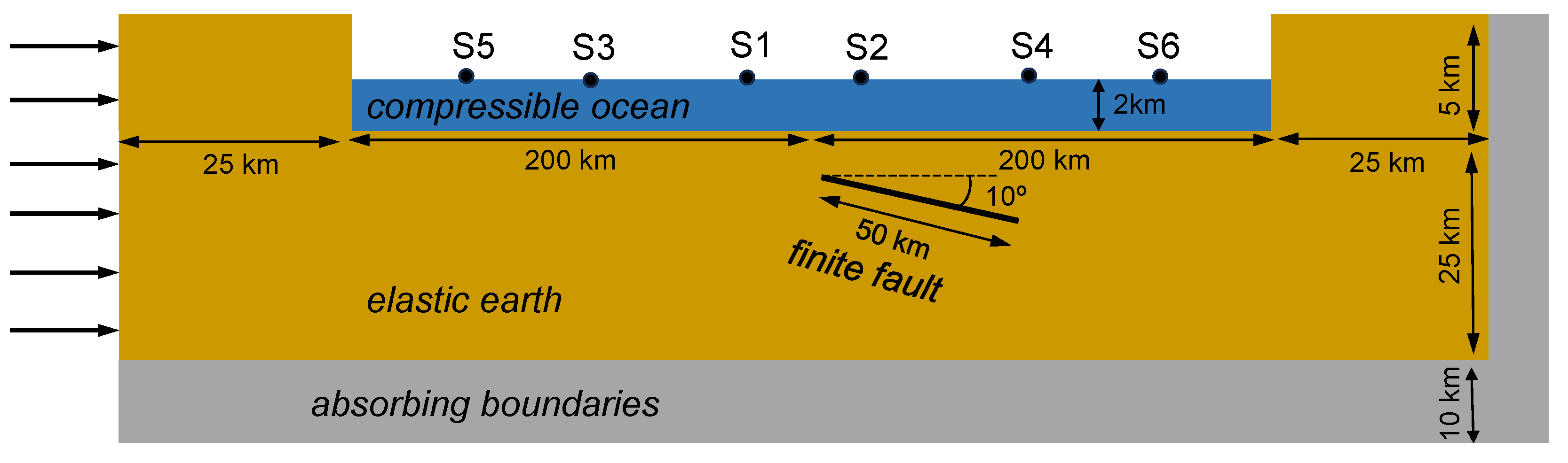
2. Numerical Generation of the Seismic and Tsunami Waves and Their Decoupling

To simulate the seismic and tsunami waves in the source region, we will separately simulate the seismic waves and the tsunami waves, and then superimpose them. Thus, it is essential to first demonstrate that seismic and tsunami waves are decoupled during the earthquake rupture process, ensuring the validity of their superposition. Theoretically, the seismic waves are elastic waves and the tsunami waves are gravity waves, so they are naturally decoupled.

To demonstrate the decoupling, we first utilize the ADINA version 9.7 (Automatic Dynamic Incremental Nonlinear Analysis) finite element software [29] to establish a tsunami generation model, as illustrated in Figure 1. In the model, the blue region represents seawater, while the yellow region represents the solid Earth structure. In the seawater, we have the density ${\rho }_0=1$${\mathrm{g}/\mathrm{cm}}^3$ and the bulk modulus $K=2.16$ $\mathrm{GPa}$, while in the solid, we have the density ${\rho }_s=2.7$${\mathrm{g}/\mathrm{cm}}^3$, the shear modulus $\mu =32$ $\mathrm{GPa}$, and the Poisson’s ratio $\nu =0.25$. A finite fault with a dip angle of 10^∘ was defined within the solid region. The top of the fault is 2 km below the seafloor. Absorbing boundaries with a thickness of 10 km were applied at the bottom and lateral sides of the model to mitigate the influence of seismic wave reflections.

We applied gravitational loading to the entire fluid and solid regions. We then applied a horizontal displacement load of 800 m to the left boundary of the model to induce sliding along the fault and trigger a tsunami [30,31] The simulation has two steps. In the first step, it calculates the static response of the whole model under the 800-m loading on the left boundary. In the second step, we weaken the elastic properties in the fault zone, i.e., the shear modulus inside the fault zone is reduced from 32 GPa to 0.32 GPa. As a result of the material weakening and residual stress, the fault dislocates and generates an earthquake and tsunami. We adopt such a two-step procedure with the purpose of simulating an earthquake that ruptures naturally, without prescribing earthquake rupture parameters. The dislocation along the fault is shown in Figure 2a. Six stations were deployed at distances of 5 km, 70 km, and 120 km on either side of the fault’s upper corner, with S1 and S2 at 5 km, S3 and S4 at 70 km, and S5 and S6 at 120 km, as shown in Figure 1. At these stations, we recorded and analyzed the vertical displacement as shown later. We adopted a mesh grid size of 250 m for the model and the entire simulation was conducted with a time step interval of 1s, covering a total time step of 2000 s.

To demonstrate the decoupling of tsunami waves and seismic waves, we develop an equivalent tsunami model based on the above ADINA tsunami generation model and simulate the resulting tsunami waves using the PCOMCOT version 2.1 (Parallelized COMCOT) program [32,33,34]. We use the permanent seafloor deformation in the ADINA model for tsunami simulation in PCOMCOT. The distribution of permanent seafloor deformation in the ADINA model after seismic waves have propagated away is shown in Figure 2b. This seafloor deformation is extended 600 km in both the front and rear directions and the entire permanent deformation is further extended 400 km in both the left and right directions, forming a square tsunami simulation domain with a total length and width of 1200 km × 1200 km to establish the computational domain for the equivalent PCOMCOT model, as shown in Figure 2c. The initial water elevation, obtained by applying the Kajiura filter [35,36] to the permanent seafloor deformation, is presented in Figure 2d. The cross-section of the initial water elevation is also shown in Figure 2b for comparison with the seafloor deformation. This initial water elevation serves as the initial condition for tsunami wave simulation in the PCOMCOT program and represents the initial water elevation equivalent to that of the ADINA model. At the same time, we ensure that the parameters used for tsunami simulation in the PCOMCOT program are consistent with those in the ADINA model: the grid size is set to 250 m, the time step remains 1s and the position of the six stations.

The free surface displacement at these six stations, simulated using the ADINA model and the PCOMCOT model, are compared in Figure 3. The stations S1 and S2 are located within the source region. From Figure 3a,b, it is evident that seismic waves and tsunami waves are generated simultaneously after the earthquake. The tsunami waveforms simulated by PCOMCOT and ADINA overlap perfectly, with short-period seismic waveforms superimposed on the tsunami waveforms for the ADINA results. Figure 3c,d show that at stations S3 and S4, the seismic waves and tsunami waves begin to separate. Within the first 400 s, there are still seismic waves superimposed on tsunami waves. After 500 s, the tsunami waveforms simulated by ADINA and PCOMCOT are almost identical. After 800 s, trailing waves caused by tsunami wave dispersion become noticeable. From Figure 3e,f, at stations S5 and S6 located 120 km away from the source region, the faster-propagating seismic waves appear first, followed by the slower-propagating tsunami waves with longer periods, and seismic waves and tsunami waves are fully separated after approximately 700 s. The PCOMCOT model produces tsunami waveforms that perfectly match those simulated by ADINA model, and the free surface displacement induced by seismic waves and tsunami waves can be separated in the far field. It indicates that seismic waves and tsunami waves are decoupled, and we can separately simulate them and superimpose them to mimic a realistic observation.

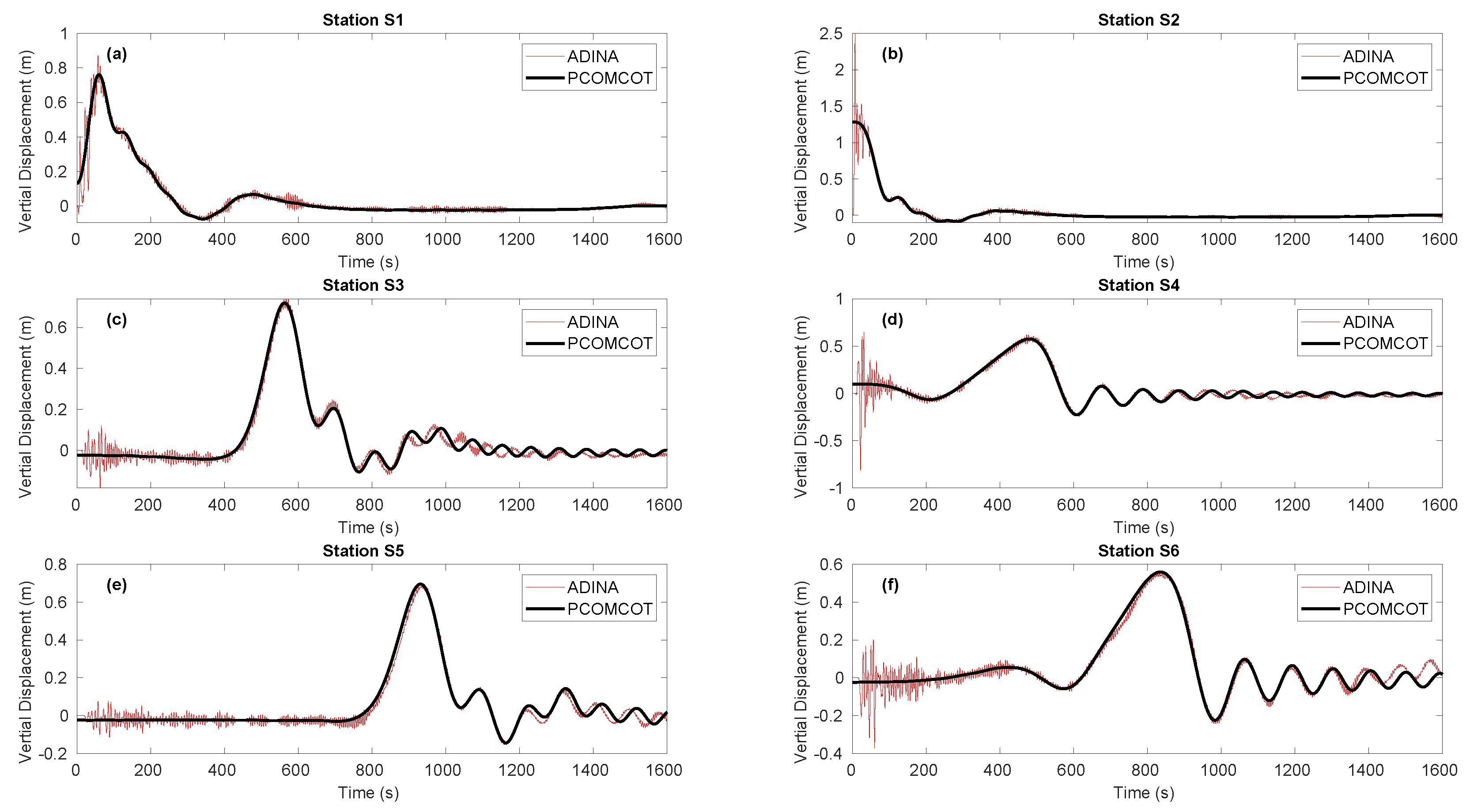
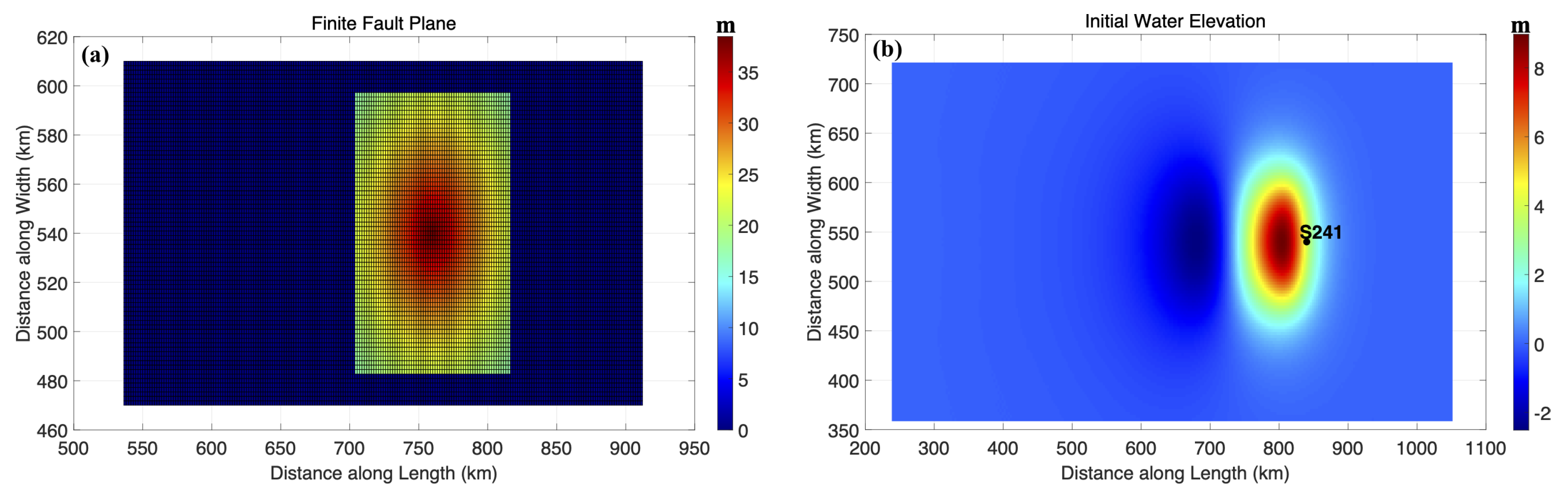
3. Simulation of Synthetic Seismic and Tsunami Waves

Given the high computational cost and storage demands of the three-dimensional ADINA tsunami generation model, and the decoupled nature of seismic and tsunami processes, we simulate these processes independently. We first use the SPECFEM 3D program [37,38] to simulate the seismic waves. The resulting tsunami initial conditions derived from the earthquake simulation are then put into the PCOMCOT program to simulate the tsunami waves. Finally, we superimpose the seismic and tsunami waves to reconstruct the coupled signals as they coexist throughout the entire seismic tsunami generation process.

We constructed the three-dimensional seismic model shown in Figure 4 in the SPECFEM3D program. The model has a total length of 1380 km, a width of 1080 km, and a water depth of 3 km, with the elastic solid extending to a depth of 600 km. The dimension of the model is large in order to avoid wave reflections at model boundaries. In the seawater, we have the density ${\rho }_0=1$${\mathrm{g}/\mathrm{cm}}^3$, and the P-wave speed $c_0=1500$$\mathrm{m}/\mathrm{s}$, while in the solid, we have the density ${\rho }_s=3.2$${\mathrm{g}/\mathrm{cm}}^3$, the P-wave speed $c_p=6500$$\mathrm{m}/\mathrm{s}$, and the S-wave speed $c_s=3000$$\mathrm{m}/\mathrm{s}$.

In the solid domain, we define a thrust fault plane with a dip angle of 20^∘ and a strike angle of 180^∘. The fault’s strike is perpendicular to the vertical central plane of the model. The fault plane is defined with dimensions of 140 km in length and 400 km in width, divided into 16,940 subfaults, with a dimension of $1.8\times 1.8$ km. Note that only a portion of the fault plane is ruptured during the simulation, as shown in Figure 5a. Each subfault is approximated by a point source at its center, ensuring the total seismic moment of all subfaults matches the given seismic moment. Different scaling relations have been proposed by numerous previous studies [32,39,40,41,42]. The scaling relation we use here is proposed by An et al. [32]: $S=2.89\times {10}^{-11}{M}_0^{2/3}$, where S is the rupture area (km²) with major slip for generating tsunami waves, $M_0$ is the seismic moment (Nm), and the aspect ratio is 1:1. For an Mw 8.6 earthquake, the rupture area is 115 km × 115 km, as shown in Figure 5a. The slip distribution within the fault plane is prescribed following a Gaussian function profile from the center of the rupture area. We assume that the rupture of the fault plane starts from the subfault located at the center of the rupture area, propagating outward at a speed of 1.5 km/s. Note that the rupture speed is relatively low for a typical earthquake, but it does not affect the analysis later in this study. The half-duration of the point source at the center of each subfault is set to 1 s.

Using the SPECFEM 3D program, we simulated the earthquake process for an Mw 8.6 earthquake, with the rupture area centered at a depth of 60 km. The stations are distributed on the entire seafloor, with a spacing of 3 km between each station. The simulation employed a grid size of 3 km, a time step of 0.04 s, and a total duration of 320 s. We note that megathrust earthquakes generally have shallower depth than 60 km. In the Supplementary Information, we provide the results for a shallow thrust earthquake whose rupture area reaches the seafloor. Although the shallow earthquake has a relatively smaller magnitude of Mw 7.4, it shows that the analysis and results are very similar.

In the SPECFEM3D program gravity is ignored. As a result, the initial water elevation at the sea surface (as shown in Figure 5b) does not propagate to form tsunami waves. Thus, we constructed a model in the PCOMCOT program with the same grid size and dimension as the SPECFEM3D seismic model. Using the initial water elevation from Figure 5b as the initial condition, we simulated the tsunami waves generated by the earthquake in PCOMCOT program, covering a total duration of 6000 s. Finally, we combined the seafloor pressure signals simulated by the SPECFEM3D and PCOMCOT programs.

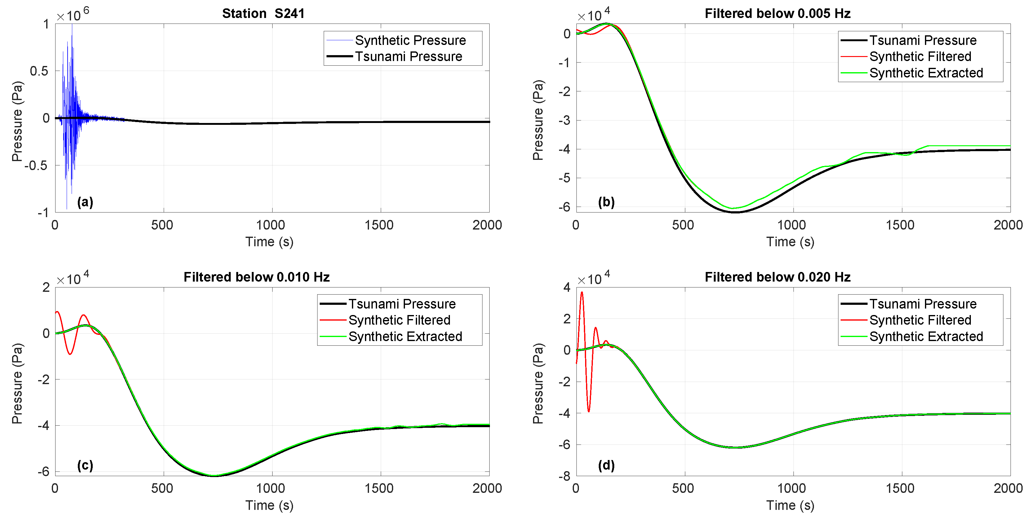
4. Extraction of Tsunami Signals

Since seismic waves and tsunami waves are already well separated at stations far from the source area, we extract tsunami signals from the coupled seismic-tsunami signals recorded at stations within the source region, for the purpose of rapid warnings. For the aforementioned Mw 8.6 earthquake, we take station S241 as an example, which is located on the seafloor within the source region, with coordinates $x=840$$\mathrm{km}$, $y=540$$\mathrm{km}$, $z=-3$$\mathrm{km}$, as illustrated in Figure 5b. The synthetic pressure recorded at this station is shown in Figure 6a. The black line in Figure 6a is the pressure from tsunami waves simulated by PCOMCOT.

Tsunami waves have low frequencies, while seismic waves are dominated by higher frequencies [9,43,44,45]. To extract tsunami signals, it is natural to apply a low-pass filter in order to extract the tsunami waves. In order to obtain the tsunami waves from the synthetic waves, we apply a low-pass filter with different cutoff frequencies. From Figure 6b, it can be seen that when the synthetic pressure signal is filtered below 0.005 Hz, the resulting filtered pressure signal (red line) shows a slightly smaller maximum tsunami amplitude compared to the original tsunami pressure signal simulated by PCOMCOT (black line). This indicates that using a low cutoff frequency will filter the seismic waves, but the tsunami signal is also affected. Consequently, the resulting tsunami signal cannot accurately reflect the true tsunami wave amplitude.

If the cutoff frequency is higher (0.01 Hz and 0.02 Hz), the filtered pressure signal (red line) still contains some seismic waves, as shown in Figure 6c,d. Here we propose that the remaining seismic waves can be removed by using a theoretical relationship between ocean-bottom pressure and vertical acceleration for seismic waves. For low-frequency seismic waves, i.e., the frequency is much lower than the resonant frequency of the water layer ($c/4h$, c water sound speed, h water depth), the ocean-bottom pressure p and the vertical seafloor acceleration a satisfy [46,47,48]

$$p=\rho ha.$$

(1)

Thus, using the seafloor acceleration recorded by a seismometer at the same site, it is able to predict the pressure caused by seismic waves using $p=\rho ha$, which is then subtracted from the total pressure to only preserve the tsunami waves. So the procedure to extract clean tsunami waves is described as follows. First, we choose a cutoff frequency to filter the pressure p and seafloor acceleration a and obtain $p_{filter}$ and $a_{filter}$. The cutoff frequency is high enough not to affect the tsunami waves, and it is also low enough in order for equation $p=\rho ha$ to be valid (much smaller than $c/4h$). In this example, it can be 0.01 Hz or 0.02 Hz, as shown in Figure 6c,d. We point out that the cutoff frequency should be chosen depending on the water depth. Numerical tests and real observations [47] indicate that equation $p=\rho ha$ is valid if the frequency is roughly lower than half of the resonant frequency. In this study, the water depth is 3000 m, and the resonant frequency is $c/4h=0.125$ Hz, and we choose a conservative value of $0.01-0.02$ Hz. After filtering, we subtract the seismic waves from the result, i.e., $p_{filter}-\rho h{a}_{filter}$, and the tsunami waves remain. Results are provided in Figure 6c,d, showing that the extracted tsunami waves perfectly match the results simulated from PCOMCOT. Thus, it is demonstrated that if filtering does not completely remove the seismic waves, it is feasible to further remove the remaining seismic waves by subtracting a prediction from the seafloor acceleration.

We point out that the first step of the method uses acausal filters, which do not cause signal time delays but require complete recordings. Thus, for real-time tsunami warnings, the method is applicable after a station records a complete tsunami waveform. For a progressive extract of tsunami waves in real time, other methods such as ensemble empirical mode decomposition (EEMD) should be considered [27]. Additionally, in this study, we demonstrate the procedure using idealized uniform bathymetry. Whether the method is applicable to a real event depends on whether equation $p=\rho ha$ holds for real bathymetry. Although the equation was theoretically derived for uniform water depth, many previous studies [46,47,49,50] have demonstrated using in situ observations that it is valid in different regions with different bathymetry, such as near Japan, Alaska, Italy, etc. Thus, it is indicated that the procedure can be applied to a real event in real bathymetry.

5. Conclusions

In this paper, we first showed that the seismic and tsunami waves are decoupled during the tsunami generation process. Therefore, we used the SPECFEM3D and PCOMCOT programs to simulate the seismic and tsunami waves separately, and the results are linearly superimposed as synthetic observations. To extract the tsunami waves from the synthetic data, only applying a low-pass filter does not completely remove the seismic waves. Thus, we proposed that the remaining seismic waves can be further removed by subtracting a prediction using a theoretical equation between ocean-bottom pressure and seafloor acceleration. The results indicate that filtering the synthetic seafloor pressure signals to the range below 0.01 Hz to 0.02 Hz preserves the complete tsunami signal. Furthermore, by subtracting the low-frequency seismic pressure component from the filtered tsunami signal, we can extract a clean tsunami pressure signal. The extracted tsunami signals allow us to determine the tsunami wave height within the source region, and are valuable for rapid tsunami warning and earthquake source characterization.

References

1. Maeda, T.; Furumura, T. FDM simulation of seismic waves, ocean acoustic waves, and tsunamis based on tsunami-coupled equations of motion. Pure Appl. Geophys. 2013, 170, 109–127. [Google Scholar] [CrossRef]
2. Lotto, G.C.; Dunham, E.M. High-order finite difference modeling of tsunami generation in a compressible ocean from offshore earthquakes. Comput. Geosci. 2015, 19, 327–340. [Google Scholar] [CrossRef]
3. Nosov, M.A.; Kolesov, S.V. Combined numerical model of tsunami. Math. Model. Comput. Simulations 2019, 11, 679–689. [Google Scholar] [CrossRef]
4. Nosov, M.; Kolesov, S. Elastic oscillations of water column in the 2003 Tokachi-oki tsunami source: In-situ measurements and 3-D numerical modelling. Nat. Hazards Earth Syst. Sci. 2007, 7, 243–249. [Google Scholar] [CrossRef]
5. Lotto, G.C.; Jeppson, T.N.; Dunham, E.M. Fully coupled simulations of megathrust earthquakes and tsunamis in the Japan Trench, Nankai Trough, and Cascadia Subduction Zone. Pure Appl. Geophys. 2019, 176, 4009–4041. [Google Scholar] [CrossRef]
6. Kanamori, H. Mechanism of tsunami earthquakes. Phys. Earth Planet. Inter. 1972, 6, 346–359. [Google Scholar] [CrossRef]
7. Saito, T. Tsunami Generation and Propagation; Springer: Berlin/Heidelberg, Germany, 2019. [Google Scholar]
8. Ben-Menahem, A.; Smith, S.W.; Teng, T.L. A procedure for source studies from spectrums of long-period seismic body waves. Bull. Seismol. Soc. Am. 1965, 55, 203–235. [Google Scholar] [CrossRef]
9. Boxberger, T.; Picozzi, M.; Parolai, S. Shallow geology characterization using Rayleigh and Love wave dispersion curves derived from seismic noise array measurements. J. Appl. Geophys. 2011, 75, 345–354. [Google Scholar] [CrossRef]
10. An, C.; Liu, P.L.F. Characteristics of leading tsunami waves generated in three recent tsunami events. J. Earthq. Tsunami 2014, 8, 1440001. [Google Scholar] [CrossRef]
11. Titov, V.V.; Gonzalez, F.I.; Bernard, E.; Eble, M.C.; Mofjeld, H.O.; Newman, J.C.; Venturato, A.J. Real-time tsunami forecasting: Challenges and solutions. Nat. Hazards 2005, 35, 35–41. [Google Scholar] [CrossRef]
12. Lay, T.; Wallace, T.C. Modern Global Seismology; Elsevier: Amsterdam, The Netherlands, 1995. [Google Scholar]
13. Satake, K. Tsunamis. In International Geophysics; Elsevier: Amsterdam, The Netherlands, 2002; Volume 81, pp. 437–451. [Google Scholar]
14. Kubota, T.; Hino, R.; Inazu, D.; Ito, Y.; Iinuma, T. Complicated rupture process of the Mw 7.0 intraslab strike-slip earthquake in the Tohoku region on 10 July 2011 revealed by near-field pressure records. Geophys. Res. Lett. 2015, 42, 9733–9739. [Google Scholar] [CrossRef]
15. Ho, T.C.; Satake, K.; Watada, S.; Fujii, Y. Source estimate for the 1960 Chile earthquake from joint inversion of geodetic and transoceanic tsunami data. J. Geophys. Res. Solid Earth 2019, 124, 2812–2828. [Google Scholar] [CrossRef]
16. Iwasaki, T.; Horikawa, K. Tsunami caused by Chile earthquake in May, 1960 and outline of disasters in northeastern coasts of Japan. Coast. Eng. Jpn. 1960, 3, 33–48. [Google Scholar] [CrossRef]
17. Levin, B.W.; Nosov, M. Physics of Tsunamis; Springer: Berlin/Heidelberg, Germany, 2009; Volume 327. [Google Scholar]
18. Kassaras, I.; Kazantzidou-Firtinidou, D. Tectonic hazards: Earthquakes. J. Environ. Hazards Methodol. Risk Assess. Manag. 2017, 7, 378. [Google Scholar]
19. Woo, G. Downward counterfactual search for extreme events. Front. Earth Sci. 2019, 7, 340. [Google Scholar] [CrossRef]
20. Goda, K.; Abilova, K. Tsunami hazard warning and risk prediction based on inaccurate earthquake source parameters. Nat. Hazards Earth Syst. Sci. 2016, 16, 577–593. [Google Scholar] [CrossRef]
21. Uchida, N.; Bürgmann, R. A decade of lessons learned from the 2011 Tohoku-Oki earthquake. Rev. Geophys. 2021, 59, e2020RG000713. [Google Scholar] [CrossRef]
22. Song, L.; An, C. Finite-fault Slip Distribution and Initial Water Elevation of the 2024 Noto Peninsula, Japan Earthquake Estimated from Tsunami Waveforms. J. Earthq. Tsunami 2024, 2450033. [Google Scholar] [CrossRef]
23. Fujii, Y.; Satake, K. Slip distribution of the 2024 Noto Peninsula earthquake (MJMA 7.6) estimated from tsunami waveforms and GNSS data. Earth Planets Space 2024, 76, 44. [Google Scholar] [CrossRef]
24. Pakoksung, K.; Suppasri, A.; Imamura, F. Preliminary modeling and analysis of the Tsunami generated by the 2024 Noto Peninsula earthquake on 1 January: Wave characteristics in the Sea of Japan. Ocean. Eng. 2024, 307, 118172. [Google Scholar] [CrossRef]
25. Shirai, T.; Enomoto, Y.; Haga, K.; Tokuta, T.; Arikawa, T.; Mori, N.; Imamura, F. Potential for tsunami detection via CCTV cameras in northeastern Toyama Prefecture, Japan, following the 2024 Noto Peninsula earthquake. Geosci. Lett. 2024, 11, 28. [Google Scholar] [CrossRef]
26. Mulia, I.E.; Gusman, A.R.; Heidarzadeh, M.; Satake, K. Sensitivity of Tsunami Data to the Up-Dip Extent of the July 2021 Mw 8.2 Alaska Earthquake. Seismol. Soc. Am. 2022, 93, 1992–2003. [Google Scholar] [CrossRef]
27. Wang, Y.; Satake, K.; Maeda, T.; Shinohara, M.; Sakai, S. A method of real-time tsunami detection using ensemble empirical mode decomposition. Seismol. Res. Lett. 2020, 91, 2851–2861. [Google Scholar] [CrossRef]
28. Kubota, T.; Saito, T.; Tsushima, H.; Hino, R.; Ohta, Y.; Suzuki, S.; Inazu, D. Extracting near-field seismograms from ocean-bottom pressure gauge inside the focal area: Application to the 2011 Mw 9.1 Tohoku-Oki earthquake. Geophys. Res. Lett. 2021, 48, e2020GL091664. [Google Scholar] [CrossRef]
29. Bathe, K.J. Finite elements in CAD and ADINA. Nucl. Eng. Des. 1986, 98, 57–67. [Google Scholar] [CrossRef]
30. An, C.; Cai, Y. The effect of beach slope on the tsunami run-up induced by thrust fault earthquakes. Procedia Comput. Sci. 2010, 1, 645–654. [Google Scholar] [CrossRef]
31. Hu, C.; Wu, Y.; An, C.; Liu, H. A numerical study of tsunami generation by horizontal displacement of sloping seafloor. J. Earthq. Tsunami 2020, 14, 2050018. [Google Scholar] [CrossRef]
32. An, C.; Liu, H.; Ren, Z.; Yuan, Y. Prediction of tsunami waves by uniform slip models. J. Geophys. Res. Ocean. 2018, 123, 8366–8382. [Google Scholar] [CrossRef]
33. Wang, X.; Liu, P.L.F. An analysis of 2004 Sumatra earthquake fault plane mechanisms and Indian Ocean tsunami. J. Hydraul. Res. 2006, 44, 147–154. [Google Scholar] [CrossRef]
34. Zhu, Y.; An, C.; Yu, H.; Zhang, W.; Chen, X. High-resolution tsunami hazard assessment for the Guangdong-Hong Kong-Macao Greater Bay Area based on a non-hydrostatic tsunami model. Sci. China Earth Sci. 2024, 67, 2326–2351. [Google Scholar] [CrossRef]
35. Kajiura, K.; Shuto, N. 11. TSUNAMIS. Ocean. Eng. Sci. 1990, 9, 395. [Google Scholar]
36. Saito, T. Tsunami generation: Validity and limitations of conventional theories. Geophys. J. Int. 2017, 210, 1888–1900. [Google Scholar] [CrossRef]
37. Peter, D.; Komatitsch, D.; Luo, Y.; Martin, R.; Le Goff, N.; Casarotti, E.; Le Loher, P.; Magnoni, F.; Liu, Q.; Blitz, C.; et al. Forward and adjoint simulations of seismic wave propagation on fully unstructured hexahedral meshes. Geophys. J. Int. 2011, 186, 721–739. [Google Scholar] [CrossRef]
38. Tromp, J.; Komatitsch, D.; Liu, Q. Spectral-element and adjoint methods in seismology. Commun. Comput. Phys. 2008, 3, 1–32. [Google Scholar]
39. Blaser, L.; Krüger, F.; Ohrnberger, M.; Scherbaum, F. Scaling relations of earthquake source parameter estimates with special focus on subduction environment. Bull. Seismol. Soc. Am. 2010, 100, 2914–2926. [Google Scholar] [CrossRef]
40. Murotani, S.; Miyake, H.; Koketsu, K. Scaling of characterized slip models for plate-boundary earthquakes. Earth Planets Space 2008, 60, 987–991. [Google Scholar] [CrossRef]
41. Murotani, S.; Satake, K.; Fujii, Y. Scaling relations of seismic moment, rupture area, average slip, and asperity size for M~9 subduction-zone earthquakes. Geophys. Res. Lett. 2013, 40, 5070–5074. [Google Scholar] [CrossRef]
42. Wells, D.L.; Coppersmith, K.J. New empirical relationships among magnitude, rupture length, rupture width, rupture area, and surface displacement. Bull. Seismol. Soc. Am. 1994, 84, 974–1002. [Google Scholar] [CrossRef]
43. Cormier, V.F. The effect of attenuation on seismic body waves. Bull. Seismol. Soc. Am. 1982, 72, S169–S200. [Google Scholar]
44. Mi, B.; Xia, J.; Shen, C.; Wang, L. Dispersion energy analysis of Rayleigh and Love waves in the presence of low-velocity layers in near-surface seismic surveys. Surv. Geophys. 2018, 39, 271–288. [Google Scholar] [CrossRef]
45. Rabinovich, A.B.; Eblé, M.C. Deep-ocean measurements of tsunami waves. Pure Appl. Geophys. 2015, 172, 3281–3312. [Google Scholar] [CrossRef]
46. An, C.; Cai, C.; Zheng, Y.; Meng, L.; Liu, P. Theoretical solution and applications of ocean bottom pressure induced by seismic seafloor motion. Geophys. Res. Lett. 2017, 44, 10–272. [Google Scholar] [CrossRef]
47. Deng, H.; An, C.; Cai, C.; Ren, H. Theoretical solution and applications of ocean bottom pressure induced by seismic waves at high frequencies. Geophys. Res. Lett. 2022, 49, e2021GL096952. [Google Scholar] [CrossRef]
48. Kubota, T.; Saito, T.; Suzuki, W.; Hino, R. Estimation of seismic centroid moment tensor using ocean bottom pressure gauges as seismometers. Geophys. Res. Lett. 2017, 44, 10–907. [Google Scholar] [CrossRef]
49. Nosov, M.; Karpov, V.; Kolesov, S.; Sementsov, K.; Matsumoto, H.; Kaneda, Y. Relationship between pressure variations at the ocean bottom and the acceleration of its motion during a submarine earthquake. Earth Planets Space 2018, 70, 100. [Google Scholar] [CrossRef]
50. Iannaccone, G.; Pucciarelli, G.; Guardato, S.; Donnarumma, G.P.; Macedonio, G.; Beranzoli, L. When the hydrophone works as an accelerometer. Seismol. Soc. Am. 2021, 92, 365–377. [Google Scholar] [CrossRef]
Figure 1. Schematic illustration of the two-dimensional tsunami generation model in ADINA. Six stations on the free surface are as follows: (1) two stations located 5 km to the left and right side of the fault’s upper corner, namely S1 and S2; (2) two stations located 70 km to the left and right side of the fault’s upper corner, namely S3 and S4; and (3) two stations located 120 km to the left and right side of the fault’s upper corner, namely S5 and S6.
Jmse 13 00419 g001
Figure 2. (a) Dislocation along the fault. (b) The permanent seafloor deformation of the ADINA model and the cross-section of the initial water elevation in PCOMCOT. (c) The permanent seafloor deformation used for the PCOMCOT model. (d) The initial water elevation in PCOMCOT.
Jmse 13 00419 g002
Figure 3. Comparison of vertical displacement at six stations on the free surface simulated using the ADINA model and the PCOMCOT model. The red and black lines represent the displacement simulated using the ADINA model and the PCOMCOT model, respectively.
Jmse 13 00419 g003
Figure 4. Schematic illustration of the three-dimensional seismic model and coordinate system used in SPECFEM 3D program.
Jmse 13 00419 g004
Figure 5. (a) The finite fault plane of an Mw 8.6 earthquake defined in the SPECFEM3D program. (b) The resulting initial water elevation of the Mw 8.6 earthquake. The black dot denotes the station S241 we used for tsunami signal extraction.
Jmse 13 00419 g005
Figure 6. (a) The synthetic pressure signal and tsunami pressure signal of the Mw 8.6 earthquake for station S241. (bd) Comparison of the tsunami pressure, the synthetic filtered pressure, and the synthetic extracted pressure when the cutoff frequency is 0.005 Hz, 0.01 Hz, 0.02 Hz. The blue line represents the synthesis pressure signal. The black, red, and green lines represent the tsunami pressure, the synthetic filtered pressure, and the synthetic extracted pressure, respectively.
Jmse 13 00419 g006
Disclaimer/Publisher’s Note: The statements, opinions and data contained in all publications are solely those of the individual author(s) and contributor(s) and not of MDPI and/or the editor(s). MDPI and/or the editor(s) disclaim responsibility for any injury to people or property resulting from any ideas, methods, instructions or products referred to in the content.