Enhancing Storm Wave Predictions in the Gulf of Mexico: A Study on Wind Drag Parameterization in WAVEWATCH III

Abstract

This study focuses on the significance of wind input source terms and their impact on wave generation in the wave model, WAVEWATCH III. Storm wave modeling capabilities were assessed with three different wind source term schemes ST4, ST6, and a new implementation ST6-IWD in a wave model to study Hurricane Ida (2021). A nested modeling approach was employed with high-resolution atmospheric wind forcing products obtained from the NOAA and the ECMWF. The model results were compared to field observations from NDBC buoys. One key finding indicates that the ST4 physical scheme is not necessarily suitable for modeling waves under extreme wind conditions. The ST6 and ST6-IWD schemes performed well for the hurricane scenario and the wave parameters obtained from these two sets of simulations were in good agreement with the observed values. The wind source term derived in the ST6 scheme holds good for wind speeds up to 50 m/s, whereas the drag method in ST6-IWD could remain stable up to ~113 m/s wind speeds. Therefore, this study recommends the ST6-IWD scheme, as it is suitable for more extreme hurricane wind conditions. It was also identified that the ST6-IWD method better estimates the peak wave periods and peak directions for Ida’s conditions.

1. Introduction

Coastal regions are typically highly populated due to their appeal, leading to a concentration of buildings and infrastructure near the shore. As these developmental activities are happening at a rapid pace worldwide, it is crucial to understand how various environmental conditions could impact these settlements. In particular, tropical-cyclone-induced disasters are of the highest magnitude, and the Gulf of Mexico1 (currently also known as Gulf of America) basin has faced many such events that created havoc along its coastlines. The damage caused by tropical cyclone winds, waves, storm surge, and precipitation varies between nearshore and offshore regions. A recent report by the National Oceanic and Atmospheric Administration (NOAA) states that, out of all natural disasters, tropical cyclones caused the greatest damage in terms of casualties and costs in the United States. Between 1980 and 2024 (as of 1 November 2024), tropical cyclones induced a death toll of around 7201, and the total cost of damages reached an exorbitant figure of USD 1.425 trillion [2].

Understanding the extreme winds and waves associated with tropical cyclone events is very important to plan and execute efficient mitigation strategies. Advanced modeling and forecasting techniques have been developed and implemented by different agencies at an operational level in recent decades. The accuracy of the modeled waves is highly dependent on the wind forcing provided to the model during the simulations. For extreme weather events such as tropical cyclones/hurricanes, the atmospheric forcing should have the capacity to capture the hurricane’s peak wind speeds and their relative directions with an accurate profile [3,4,5]. Discrepancies in any atmospheric forcing will directly translate to the waves, producing inaccuracies in estimates. Therefore, it is very important to identify and use an atmospheric model that produces reliable predictions of hurricane wind conditions [6]. The accuracy of wave models is also highly dependent on their source terms (especially in third-generation wave models) such as wind drag, bottom friction, and non-linear quadruplet wave interactions. Most wave models struggle to generate reliable estimates of waves under extreme wind conditions due to the high parameterization of these source terms [7]. The wind drag coefficient (C_d) is one of the significant source terms in wave models and plays a very important role in accurate estimations of wave heights and other wave parameters [8,9]. In traditional boundary layer theory, the drag coefficient (C_d) depends on the Reynolds number when the ocean surface is smooth and on the roughness length when the surface is rough. The roughness length of the ocean surface is predominantly influenced by the surface wave conditions, which are driven by atmospheric forcings. Over the years, many researchers [10,11,12,13,14,15,16] have developed different linear bulk formulations to compute C_d as a function of wind speed. Until recently, most numerical wave models utilized one of these methods to compute the wind input source term. However, different studies started exhibiting that the wind drag does not linearly increase with the increase in wind speed, but it attains a neutral state around wind speeds between 30 and 35 m/s and even decreases at wind speeds beyond 50 m/s [17,18,19,20,21,22].

Furthermore, there are studies that focused on developing wind drag methods based on the concept of air–sea momentum exchange between the boundary layers [23,24,25,26,27,28,29,30,31,32,33]. Hara and Belcher [25,26] introduced a Wave Boundary Layer (WBL) concept that computes the wind drag and roughness heights for extreme wind conditions. This model was further enhanced by Chen and Yu [34,35] by including the sea-spray effect in the Wave Boundary Layer Model (WBLM), which brought the decreasing tendency in C_d for high wind speeds. This was further validated by Shankar and Behera [8,9,36] through the application of the WBLM method in the Bay of Bengal basin for computing storm wave and surge. Although the WBLM estimates the drag in good correlation to field and experimental values, it is a tedious and computationally expensive method. Shankar and Behera [9] developed an Improved Wind Drag (IWD) method based on the WBLM concept and studied it for two extreme hurricanes Katrina (2005) and Rita (2005) that made landfall in the Gulf of Mexico basin. The IWD method gave promising results for water levels and wave heights when introduced into the coupled Advanced Circulation model (ADCIRC) [37] and Simulating Waves Nearshore model (SWAN) [38].

WAVEWATCH III (WW3) [39] is one of the third-generation wave models used to generate ocean surface waves, which are primarily driven by atmospheric forcing (wind velocity). WW3 is an operational wave model for the NOAA and is built with different physical schemes, namely, ST1 [40,41,42], ST2 [39,43,44], ST3 [45,46], ST4 [47], and ST6 [48,49]. Several studies have identified that ST4 is suitable for regular wind conditions [6,47,50], and the latest ST6 scheme performed well under both regular and extreme wind conditions [51,52,53]. The wind input source term (wind drag) in the physical scheme ST4 follows the relationship developed by Charnock [10] and Wu [14], whereas ST6 adopts the method introduced by Hwang [20]. The wind drag method in ST4 is a bulk linear method that computes an increasing C_d with the increase in wind speed, and a cut-off term is set to avoid unrealistic values. Hwang’s method in ST6 follows a quadratic relationship, which includes the decreasing tendency of C_d at high wind speeds. However, the method holds good until a 50 m/s wind speed, and beyond that, a constant cut-off term is set. In this study, we implement the IWD method developed by Shankar and Behera [9] into the WW3 physical scheme ST6, as the IWD method was developed through the WBLM concept, and it also performs well for extreme hurricane wind speeds beyond 80 m/s. The aim of this study is to do a comparative analysis between ST4, ST6, and ST6-IWD and identify a suitable wind drag method for storm wave modeling. Hurricane Ida (2021), which made landfall along the Louisiana coastline of the United States, was chosen to be modeled using WW3 for all three conditions (ST4, ST6, and ST6-IWD). The atmospheric (wind) forcing for the wave model WW3 was obtained from operational NOAA High-Resolution Rapid Refresh (HRRR) and the European Centre for Medium-Range Weather Forecasts (ECMWF) datasets. The overall focus of this work is to gain an enhanced understanding of the sensitivity of the wind drag coefficient in terms of hurricane wind wave modeling.

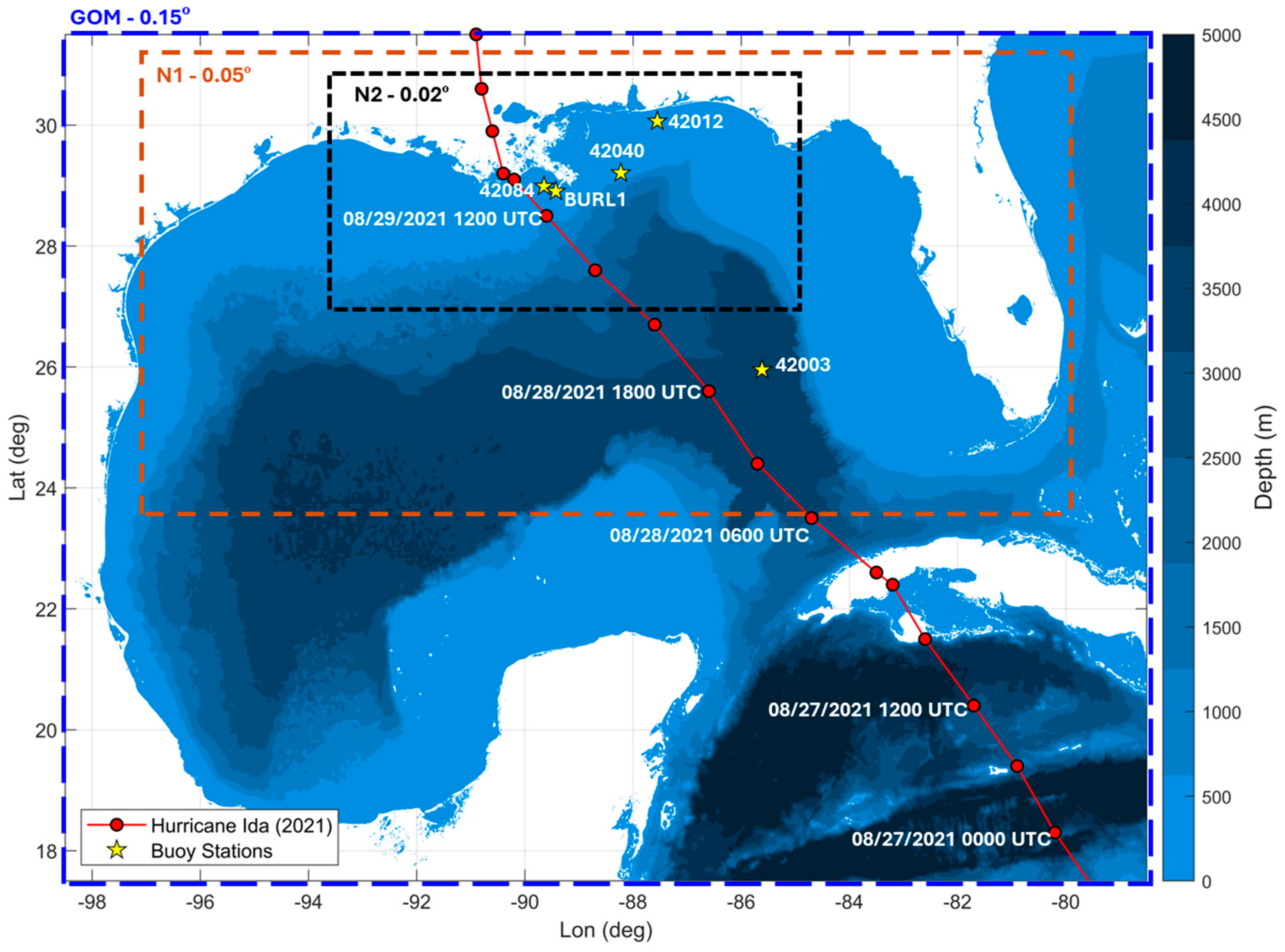
2. Hurricane Ida Description

Hurricane Ida formed through the combination of several low-latitude systems that began with a tropical wave emerging off the African coast on 14 August 2021 and moved towards the western Caribbean Sea on 23 August 2021 [1]. Initially, this weak wave was difficult to track while moving across the eastern Atlantic. By 12:00 UTC on 26 August 2021, the system had developed into a tropical depression, located approximately 150 nautical miles southwest of Kingston, Jamaica. Around 1800 UTC on 27 August 2021, the system had rapidly intensified into a tropical storm and then a hurricane, achieving wind speeds of 70 knots as it approached the Isle of Youth, Cuba. Continuing northwest, Ida entered the Gulf of Mexico (GOM) basin [1] between 01:00 and 02:00 UTC on 28 August 2021, where it rapidly intensified due to the warm waters present in the Gulf. Ida reached peak wind speeds of 66.88 m/s (130 knots) during landfall at 16:55 UTC on 29 August 2021, at Port Fourchon, Louisiana. At landfall, Ida was a Category 4 hurricane with an eye of a 15-nautical-mile width, causing a storm surge of approximately 4.3 m that flooded nearby coastal areas [1]. After landfall, Ida moved east–northeastward, weakening into an extratropical low system and bringing significant rainfall to land. Hurricane Ida was responsible for a total of 96 casualties (direct and indirect), and the total cost of the damage was estimated to be around USD 84.6 billion [54].

3. Data and Methodology

3.1. Atmospheric Forcing

In this study we utilize the wind data obtained from the NOAA/NCEPs (National Centers for Environmental Predictions) and the ECMWF as the atmospheric forcings into the wave model to generate waves. The wind data contain u10 and v10 at hourly intervals which are interpolated to the wave model grids at certain specified time steps based on wave model grid resolutions (which is elaborated in Section 3.2) and configurations. The below sections elaborate on the atmospheric forcings obtained from the corresponding agencies.

3.1.1. HRRR—High-Resolution Rapid Refresh

NOAA/NCEP introduced an innovative numerical model to the Numerical Weather Prediction forecast system in 1998, which operated on an hourly time step, unlike the existing 2 or 4 time step models of that period. This model was named the Rapid Update Cycle (RUC, [55]). In 2012, the RUC evolved into the Rapid Refresh (RAP) model to enhance accuracy, incorporating new features. RAP operates on a 13 km horizontal grid covering nearly all of North America. For a more focused regional approach in the United States, a 3 km resolution grid with 51 vertical layers (HRRR) was developed alongside RAP and became operational in 2014 [56,57]. The 3 km high-resolution HRRR domain covers the entire United States over land regions and parts of the coastal regions on all sides associated with the model domain (as shown in Figure 1 of Benjamin et al. [58]). The southern end of the HRRR model domain extends only to the northern Gulf of Mexico basin. The model is initialized using 3 km grids and incorporates radar data assimilation at the same resolution. Every 15 min, radar data are assimilated over a 1 h period, enhancing the detail provided by the hourly data assimilation from the 13 km RAP model. Initially, HRRR provided forecasts up to 18 h ahead, and with the subsequent versions of HRRRv2 (23 August 2016), HRRRv3 (12 July 2018), and HRRRv4 (2 December 2020), the forecast range was extended to 48 h. The latest version, HRRRv4, includes improvements in storm prediction near the eye and boundaries of tropical and extratropical cyclones, cloud cover representation, lake temperatures, and more [57,58,59]. In this study, the u and v components of 10 m winds were obtained for the duration of Hurricane Ida with respect to the HRRR version (v4) and were used as the primary atmospheric forcing to simulate extreme wind-generated waves in the wave model WW3.

3.1.2. ECMWF—High-Resolution Operational Forecast Model

The ECMWF offers a variety of real-time and archived atmospheric and oceanographic datasets that also include the high-resolution operational forecast model. This global forecast model operates on a horizontal grid resolution of 9 × 9 km and 137 vertical layers, providing a comprehensive range of data products that covers the entire globe [60,61]. The high-resolution model runs four times daily (0000, 0006, 0012, and 0018 h), producing 90 h forecasts ahead at each time step. Additionally, the model generates forecasts on 3-hourly and 6-hourly intervals daily, extending the forecast horizon to 93–144 h and 150–240 h, respectively. For this study, we utilized the 0000 and 0012 h time steps of the u10 and v10 variables with 11 h forecasts from the archived data, which served as the secondary atmospheric forcing for the regions that were not covered by the HRRR wind model, and the simulations for Ida were carried out.

3.2. WAVEWATCH III Configuration

We employed a nested multi-grid modeling approach [6] using WW3 to generate storm waves under the wind conditions of Hurricane Ida. The model grids and their respective resolutions are shown in Figure 1, with the Gulf of Mexico grid (GOM—0.15° × 0.15° (~16.5 km × 16.5 km)) serving as the parent grid and nests N1 (0.05° × 0.05° (~5.55 km × 5.55 km)) and N2 (0.02° × 0.02° (~2.22 km × 2.22 km)) covering the northern GOM basin and the landfall area of the Hurricane Ida, respectively. The Gridgen package from the NOAA-EMC [62,63] was used to create the WW3 model grids. The corresponding bathymetric water depths for all three wave model grids (GOM, N1, and N2) were interpolated from the global dataset provided by the General Bathymetric Chart of Oceans, which has approximately 450 m (15 arc second) resolution. The different configuration time steps for the wave model, including the maximum global time step, maximum CFL time step for x-y and k-theta, and minimum source term time step for all three model grids, were set to GOM—900 s, 450 s, 450 s, 15 s; N1—600 s, 180 s, 180 s, 10 s; and N2—90 s, 30 s, 30 s, 5 s, respectively, based on the CFL criterion. The model’s spectral frequency increased logarithmically from 1.17 to 0.0285 Hz with 24 steps, and the directional spectrum has a resolution of 10° at 36 directions. For all three case scenarios (ST4, ST6, and ST6-IWD), the initial condition was set to the Joint North Sea Wave Project (JONSWAP) spectral parametric scheme with directional distribution of the waves [64,65]. Other WW3-model-based switches, such as non-linear Discrete Interaction Approximation (DIA—NL1), SHOWEX bottom friction (BT4), wave reflection of shorelines and icebergs (REF1), Battjes–Janssen depth-induced breaking (DB1), Lumped Triad Interaction (LTA—TR1), and wind speed and current interpolations in space and time (WNT2, WNX1, CRT1, CRX1), were activated for all three wind scheme cases. To estimate the wave parameters for Hurricane Ida, two wind datasets—HRRR and the ECMWF—were utilized as atmospheric forcing in the wave model. The HRRR model, which covers only the northern Gulf and includes the N1 and N2 wave model grids, was complemented by the ECMWF dataset. The ECMWF dataset served as the secondary wind forcing for the outer GOM grid across all three scenarios. Additionally, the boundary conditions for the outer GOM domain were derived from the ECMWF’s ERA5 global reanalysis wave model dataset, which has a resolution of 0.5° × 0.5° [66].

3.3. Wind Drag Methods

As elaborated in the above sections, the WW3 model has various physical schemes for the wind input source term, and in this study, we evaluate a new implementation ST6-IWD along with the existing schemes, ST4 and ST6. This section provides brief information on the corresponding wind drag methods adopted in those physical schemes.

ST4: This physical scheme implements an analytical procedure for computing the wind drag coefficient as follows:

$${\mathrm{C}}_{\mathrm{d}}={\left({\displaystyle \frac{{\mathrm{u}}_{\ast }}{{\mathrm{u}}_{10}}}\right)}^2$$

(1)

where ${\mathrm{u}}_{\ast }$ is the wind friction velocity (m/s) and ${\mathrm{u}}_{10}$is the wind speed (m/s) at 10 m height. The wind friction velocity (${\mathrm{u}}_{\ast }$) is computed through an iterative process that loops over a range of wave-supported stress (${\tau }_w$) and ${\mathrm{u}}_{10}$ using a steady-state wind profile and the Charnock [10] relation for roughness length (${\mathrm{z}}_0$). More details on the iterative process on the computation are elaborated in [47,67]. To avoid unrealistic wind stresses at extreme wind speeds (${\mathrm{u}}_{10}$), a maximum value of 0.0015 was set for ${\mathrm{z}}_0$ to maintain a saturation-based dissipation [47].

ST6: In this scheme, the wind input source term was estimated using the method developed by Hwang [20] and is as follows:

$${\mathrm{C}}_{\mathrm{d}}\times {10}^4=8.058+0.967{\mathrm{u}}_{10}-0.0167{{\mathrm{u}}_{10}}^2$$

(2)

This is a quadratic method that holds good for ${\mathrm{u}}_{10}$ up to 50 m/s, as the data used to develop this relationship had a maximum wind speed of 50 m/s, and wind speed C_d tends to drop below zero for larger wind speeds. To avoid that, a simple modification with a bulk adjustment to the computational framework was arranged in such a way that C_d does not drop below zero [48].

ST6-IWD (Improved Wind Drag): A new implementation, where Hwang’s method in ST6 was replaced with the method proposed by Shankar and Behera [9], is as follows:

$${\mathrm{C}}_{\mathrm{d}}\times {10}^3=\left(0.42+3.86\tilde{\mathrm{u}}-2.53{\tilde{\mathrm{u}}}^2+0.4{\tilde{\mathrm{u}}}^3\right)$$

(3)

where $\tilde{\mathrm{u}}={\mathrm{u}}_{10}/{\mathrm{u}}_{\mathrm{r}\mathrm{e}\mathrm{f}}$ and ${\mathrm{u}}_{\mathrm{r}\mathrm{e}\mathrm{f}}$ is the reference wind speed (37.5 m/s) at which the drag coefficient attains its maximum value according to the method proposed by Shankar and Behera [9]. This method maintains a stable saturation for hurricanes with speeds up to ~113 m/s, and no cut-off term needs to be introduced as most hurricanes peak winds fall under 100 m/s.

4. Results and Discussion

The simulations for all three cases, ST4, ST6, and ST6-IWD, were carried out for Hurricane Ida’s conditions using the nested model setup in WW3, and the results generated (wind and wave parameters) were compared and analyzed with the in situ data obtained from different NDBC stations (shown in Figure 1). Initially, the time series of the wind speed estimated through HRRR was compared with the observed buoy data available at stations 42003, 42012, 42040, and BURL1, as displayed in Figure 2. Along with the time series comparison, the corresponding model–data scatter and the statistical error estimates such as Root Mean Square Error (RMSE), bias, scatter index (SI), and correlation coefficient (R) were also computed and demonstrated for all four stations in Figure 3. The time series indicates that the wind speed from the atmospheric model HRRR aligns well with the observations at stations 42003, 42012, and 42040. At station BURL1, which was closest to Ida’s track when it was making landfall (as shown in Figure 1), peak hurricane wind speeds reached approximately 47 m/s on August 29. However, the HRRR model underestimated these speeds, recording a peak of only 40.7 m/s. This was about a 14% underestimation between the observation and HRRR at this station, and a similar difference was also seen through the statistical error estimates (Figure 3) for this location with the highest SI and negative bias. Apart from considering the peak wind estimation at station BURL1, the statistical estimates were very promising at all the other three stations, 42003, 42012, and 42040, with higher correlation coefficients (>0.969) and lower scatter indices (<16.4%). It is important to note that the error metrics between HRRR and buoy data shown in Figure 3 exhibit high correlation coefficients (0.96–0.98) at all the stations. The negative bias at BURL1 portrays the underestimation of peak wind at this station by the atmospheric model with the lower model performance at this station also confirmed by the high scatter index. The spatial distribution of Hurricane Ida’s wind field on 29 August 2021, 1200, UTC (when Ida attained Category 4 status) along with the wind drag coefficients computed from all three methods (ST4, ST6, and ST6-IWD) is shown in Figure 4. It could be seen that the HRRR-model-based wind speeds reached a maximum of around 60 m/s, which was close to the observed range of ~66 m/s [1,6]. The drag coefficient distribution in Figure 4 displays the spatial difference in the wind drag scheme between these three methods. Overall, the hurricane wind profile was well represented in HRRR with the proper depiction of Ida’s winds in all four quadrants.

Figure 5 presents a comparison of the wind drag coefficient (C_d) obtained from three different wind input schemes at the approximate location where the maximum winds from Hurricane Ida were observed, according to HRRR data. The bottom panel of Figure 5 clearly shows that the C_d from the ST4 physical scheme generates very high wind drag coefficients at wind speeds exceeding approximately 20 m/s. An ad hoc constraint term in ST4 is designed to prevent unrealistic C_d values at high wind speeds [47]. Beyond this wind speed threshold, the stress terms are computed based on the maximum roughness length cap (0.0015) as mentioned earlier for Equation (1). The drag coefficients from ST6 and ST6-IWD, as shown in Figure 5, follow the quadratic and cubic nature of Equations (2) and (3), respectively. The ST6 drag coefficients are generally higher than those of ST6-IWD for wind speeds up to 30 m/s. At 37 m/s, the coefficients converge, but beyond this point, the ST6 coefficients drop drastically, while the ST6-IWD coefficients maintain their profile. This behavior aligns with the spatial comparison of drag coefficients depicted in Figure 4 (contour levels). In regions of maximum winds from Hurricane Ida, ST4 estimates very high drag coefficients, and ST6 shows a significant drop in C_d below 0.001 and will continue to drop for higher wind speeds. In contrast, the drag coefficient in ST6-IWD does not drop as much as in ST6, which is advantageous for storm wave modeling at extreme wind speeds.

The wave parameters were modeled for Hurricane Ida’s conditions with all three wind input source term scenarios, ST4, ST6, and ST6-IWD, and the model results were compared and analyzed against observations. To begin with, the significant wave height (Hs) time series obtained through the nested wave model for the three cases were compared at buoy locations 42003, 42012, 42040, and 42084 (depicted in Figure 6). The corresponding statistical error estimates—RMSE, bias, SI and R—were also calculated for the time series and shown in Figure 7. The modeled Hs values from all three source terms showed an overall good agreement with the in situ observations at all stations for wind speeds up to 15 m/s (28 August) in generating smaller wave heights below ~4 m, as can be seen from both the time series plots (Figure 6) and the scatter plots (Figure 7). However, discrepancies in model results and buoy observations increase as hurricane winds larger than 20 m/s approach the stations (Figure 2), and the model results for wave heights larger than 4 m tend to overestimate the observations at all stations (Figure 7). For example, at station 42003, the peak wave height observed was around 7 m, but ST4-, ST6-, and ST6-IWD-based model simulations estimated it to be around 8.1 m, 8.0 m, and 7.7 m, respectively. Out of the three schemes adopted in this study, the ST6-IWD one came closest to the observed value at this location with the smallest error of 9%. The percentage error of the peak wave height at this station for ST4 and ST6 was found to be larger at 13.6% and 12.5%, respectively. The larger error in peak wave heights in ST4 and ST6 may be attributed to their larger drag coefficients (Figure 5) leading to an overestimation of wave heights at those wind speeds captured reasonably well by HRRR.

At stations 42012 and 42040, the modeled versus observed wave heights correlated very well, as reflected in the statistical error estimates with high R (>0.988) and low RMSE (<0.039 m), and SI (<18%) values. The peak wave heights at these two stations were observed to be around 5.15 m and 8.2 m, respectively. The model-generated peak wave heights at these stations were as follows: ST4: 4.92 m and 9.1 m, ST6: 5.1 m and 9.2 m, and ST6-IWD: 5.2 m and 8.8 m. The percentage errors for these models were as follows: ST4: 4.47% (underestimation) and 10.98% (overestimation), ST6: 0.97% (underestimation) and 12.20% (overestimation), and ST6-IWD: 0.97% (overestimation) and 7.32% (overestimation). The winds are weakest at 42012 (farthest from hurricane track); therefore, ST4 produces wave heights closer to the measurements with a smaller error at this station as its drag coefficient is in line with those of ST6 and ST6-IWD (similarly to as is shown in Figure 5). On the other hand, the hurricane-forced peak winds arrive at 42040 later (29 August, Figure 2) at a magnitude similar to that of 42003 (slightly larger than 20 m/s); therefore, there is a similar reduction in error in predicting the peak wave height when ST6-IWD is used. The nearshore station 42084 was the closest to the hurricane track and could not measure the peak wave height produced by the storm. However, the second highest observed peak wave height was around 8.7 m. The second peak of 8.7 m was well captured by the ST6-IWD (8.71 m) and ST6 (8.69 m) schemes, but the ST4-based simulations underestimated it (8.3 m). The percentage errors for these models were as follows: ST4: 1.72% (underestimation), ST6: 0.11% (underestimation), and ST6-IWD: 0.11% (overestimation). At this location, the ST4-, ST6-, and ST6-IWD-computed peak modeled wave height values were 8.55 m, 9.0 m, and 9.4 m, respectively. Based on the comparisons at stations 42003, 42012, and 42040, it could be assumed that the ST6-IWD scheme’s peak wave height of 9.4 m at station 42084 could be close to the same order of magnitude that Ida generated at this station. The peak significant wave heights due to Ida’s winds spatially varied from 11 to 12 m for ST4, 12 to 13 m for ST6, and 13 to 14 m for ST6-IWD (shown in Figure 8). In general, the peak significant wave heights generated by Hurricane Ida were reported around 13 m during landfall along the Louisiana coastline [1,6]. The ST6-IWD and ST6 physical schemes, which attribute the decreasing tendency of the wind drag coefficient for higher winds, captured those peak wave heights in the wave model closer with respect to the in situ observations for Hurricane Ida. Although both these schemes perform well for hurricane conditions, the advantage of ST6-IWD over ST6 is that the former method is effective for wind speeds up to ~112 m/s (reaches negative at ~113 m/s and needs a cut-off term), while the latter is only effective up to 50 m/s, requiring a cut-off term for wind speeds beyond that.

In addition to the significant wave heights, the peak wave periods (T_p) and peak wave directions were also computed for all three case scenarios. The modeled values were compared with the buoy data and further analyses were carried out. Figure 9 presents the comparison of the time serios of the peak wave period at NDBC buoys 42003, 42012, 42040, and 42084. Irrespective of the physical schemes adopted, the modeled peak periods almost resembled one another and were in good agreement overall with the observed variations at all the locations (R up to 0.91). Apart from a brief period between 0900 August 23 and 0600 August 25 at 42003 (where it underestimates the T_p), the wave model’s performance on the peak wave period was quite accurate (RMSE as low as 0.11 s). Almost all the schemes had the same ranges of statistical error estimates, R, RMSE, bias, and SI values at all the locations (Figure 10). The brief underestimation at 42003 could be attributed to the resolution difference between HRRR (3 km—wind forcing for N1 and N2 grids) and the ECMWF (9 km—wind forcing for GOM grid), and the transition zone between these two models as the hurricane enters from one nested wave model domain to another (GOM -N1-N2). The RMSEs for the peak wave periods (Figure 10) were smallest for the ST6-IWD method, and this emphasizes the fact that ST6-IWD computes both wave heights and periods more accurately than the ST6 and ST4 methods. Wave rose diagrams created for all the stations listed above are shown in Figure 11, which displays the bins with respect to the peak wave direction, and the circles represent the frequency of those waves in that direction. Similarly to the peak wave periods, there were no significant changes noticed in the peak wave directions when the wave model was switched between the ST4, ST6, and ST6-IWD physical schemes (as represented in Figure 11). When compared with the observed data, the WW3-model-based estimations of the peak wave directions agreed well at locations 42003, 42012, and 42040. However, at 42084, a shift of 20° was noticed in the directional estimates between the models and buoy data. As this location, which was closest to the hurricane track, the wave propagation and transformation from the deep waters to the nearshore regions could have caused this shift as it entered the continental shelf. Apart from this, the estimates of the peak wave directions for the physical schemes through WW3 were in reasonable agreement when compared to the in situ data.

5. Summary and Conclusions

Storm wave modeling is a challenging task due to numerous uncertain factors affecting the accuracy of the results. One crucial factor is the wind stress component, which depends on the parameterization of the wind drag coefficient (C_d). Most wind drag schemes are linear empirical functions, which become unstable with extreme hurricane wind speeds. In this study, we analyze the wind input source terms that are inbuilt into the physical schemes (ST4 and ST6) of the wave model WAVEWATCH III (WW3) for Hurricane Ida’s conditions. Additionally, we implemented the ST6-IWD wind drag method, developed by Shankar and Behera [9], for the first time in WW3 and used it to study Hurricane Ida with a nested wave model setup for the Gulf of Mexico. The wave model was driven by the atmospheric wind forcing drawn from the NOAA/NCEPs’ High-Resolution Rapid Refresh (HRRR) model. The simulations were carried out and the results obtained from all three cases were compared with the observed data at different NDBC stations in both the near-coastal and deep waters of the Gulf of Mexico. After careful analysis of different wind and wave parameters through time series and spatial and statistical estimates, the following conclusions were drawn:

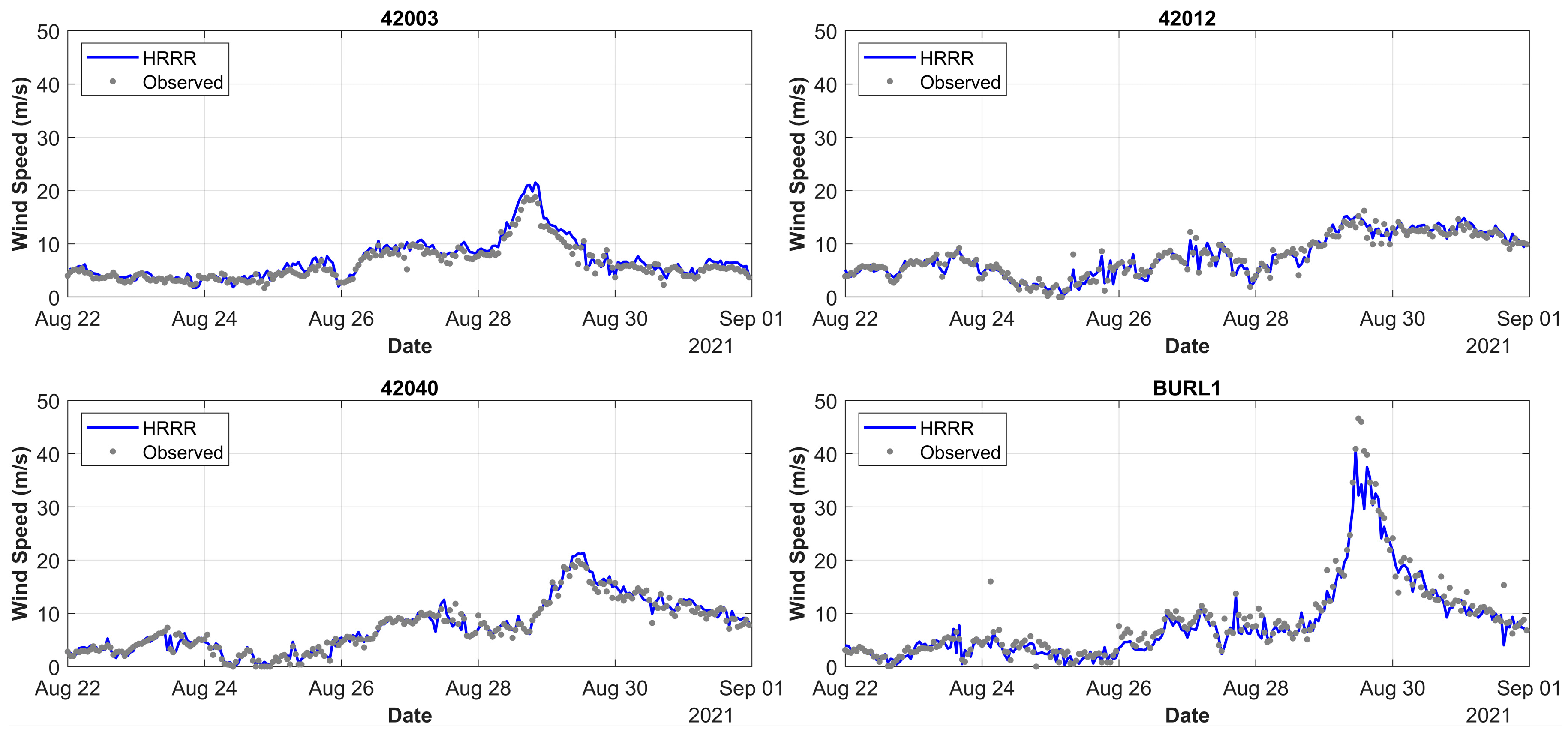
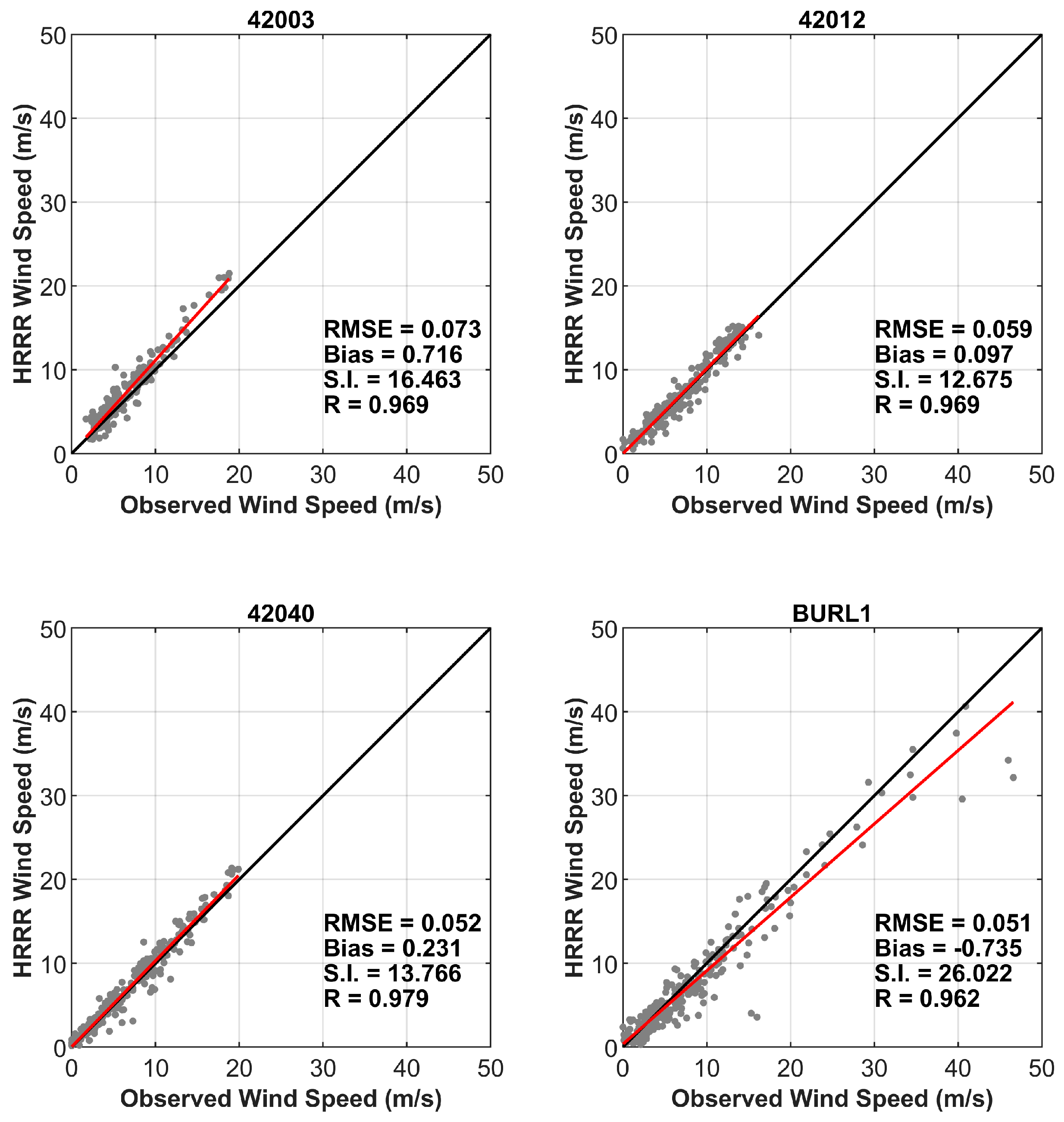
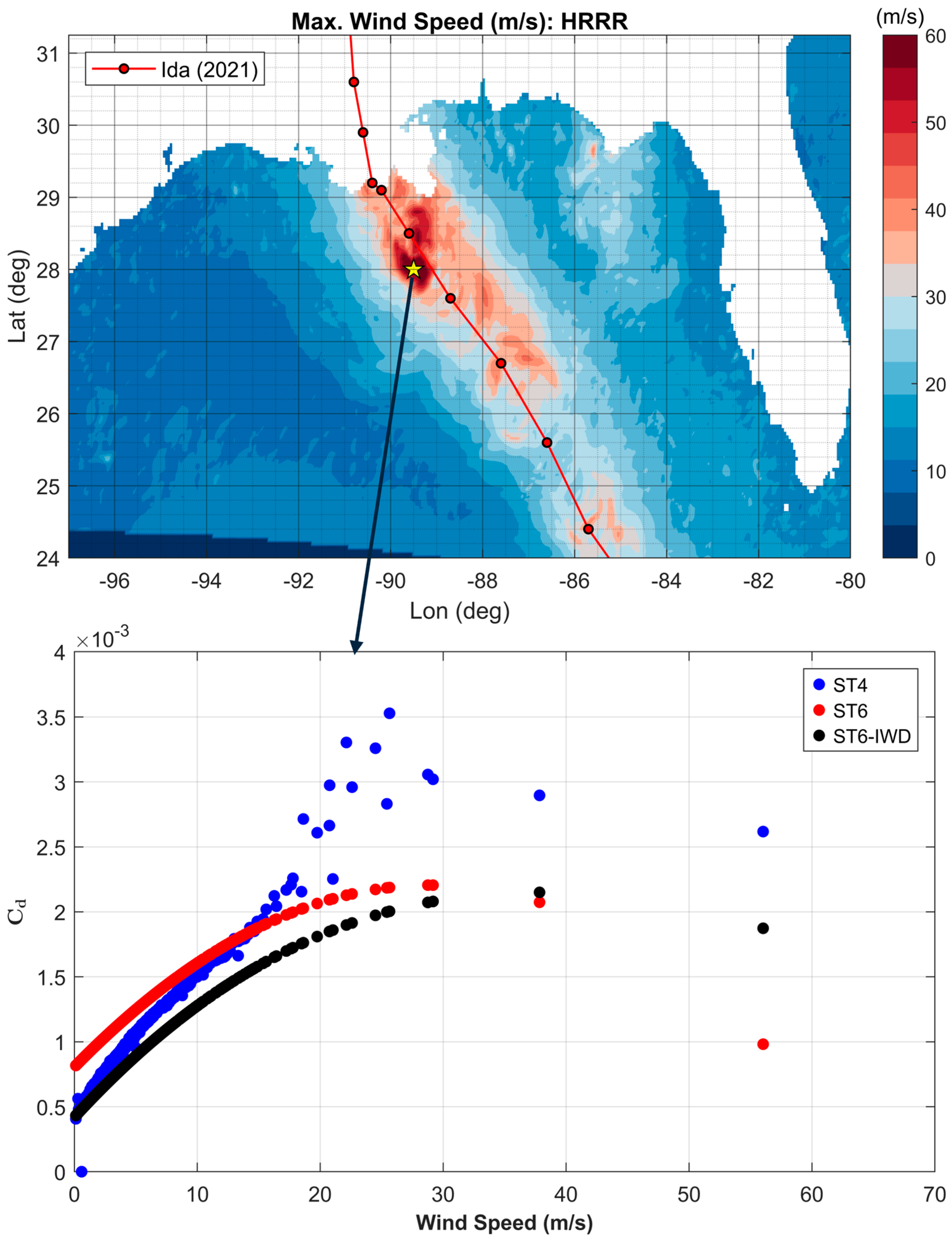
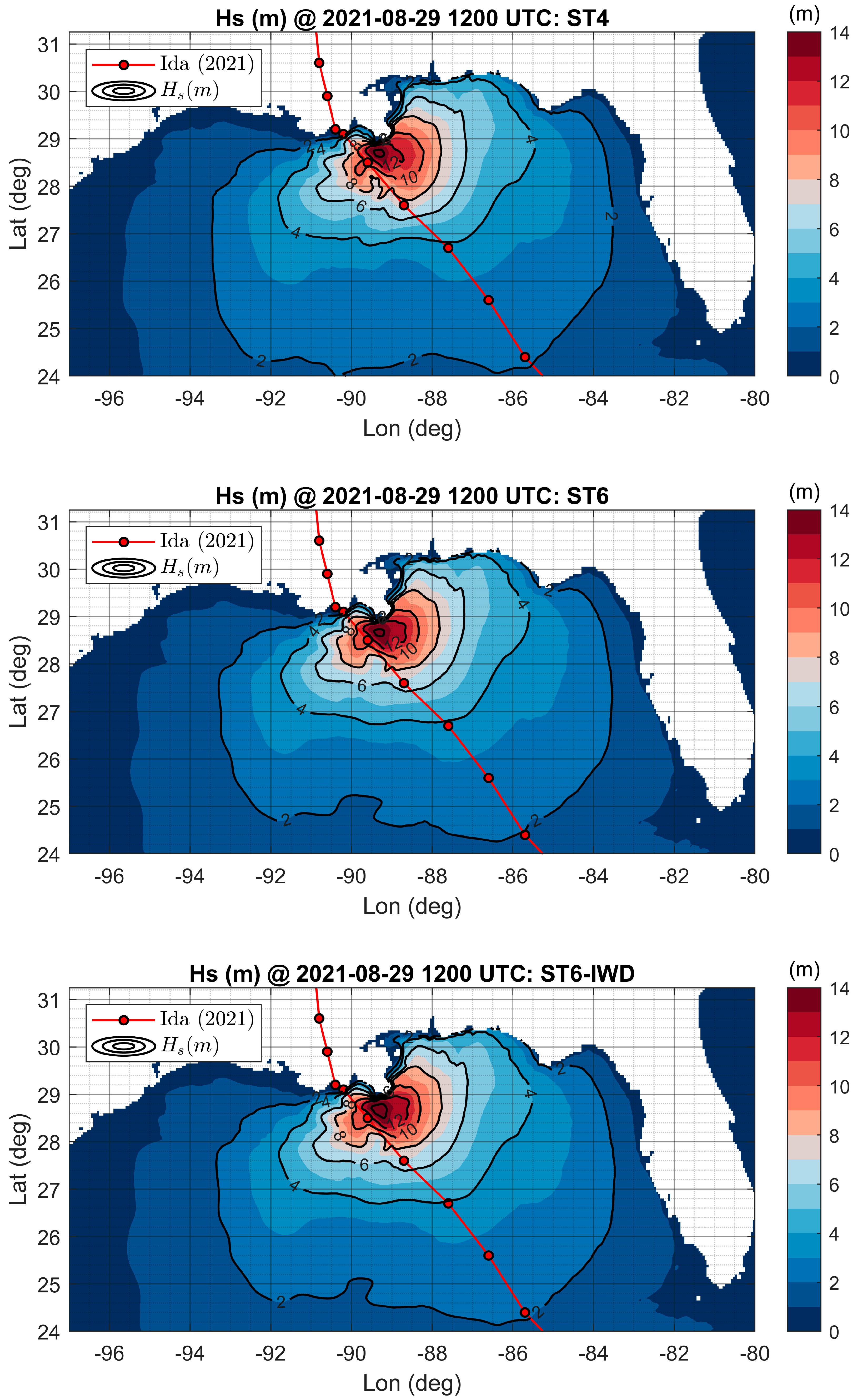
• HRRR well represented the wind speeds at buoys 42003, 42012, and 42040, where the maximum wind speeds in these locations were observed to be around 25 m/s. At the BURL1 station (closest to Ida’s track), the model underestimated the peak hurricane wind speeds by 14%. The spatial representation of the hurricane wind bands was well captured by HRRR as Hurricane Ida made landfall along the Louisiana coastline.
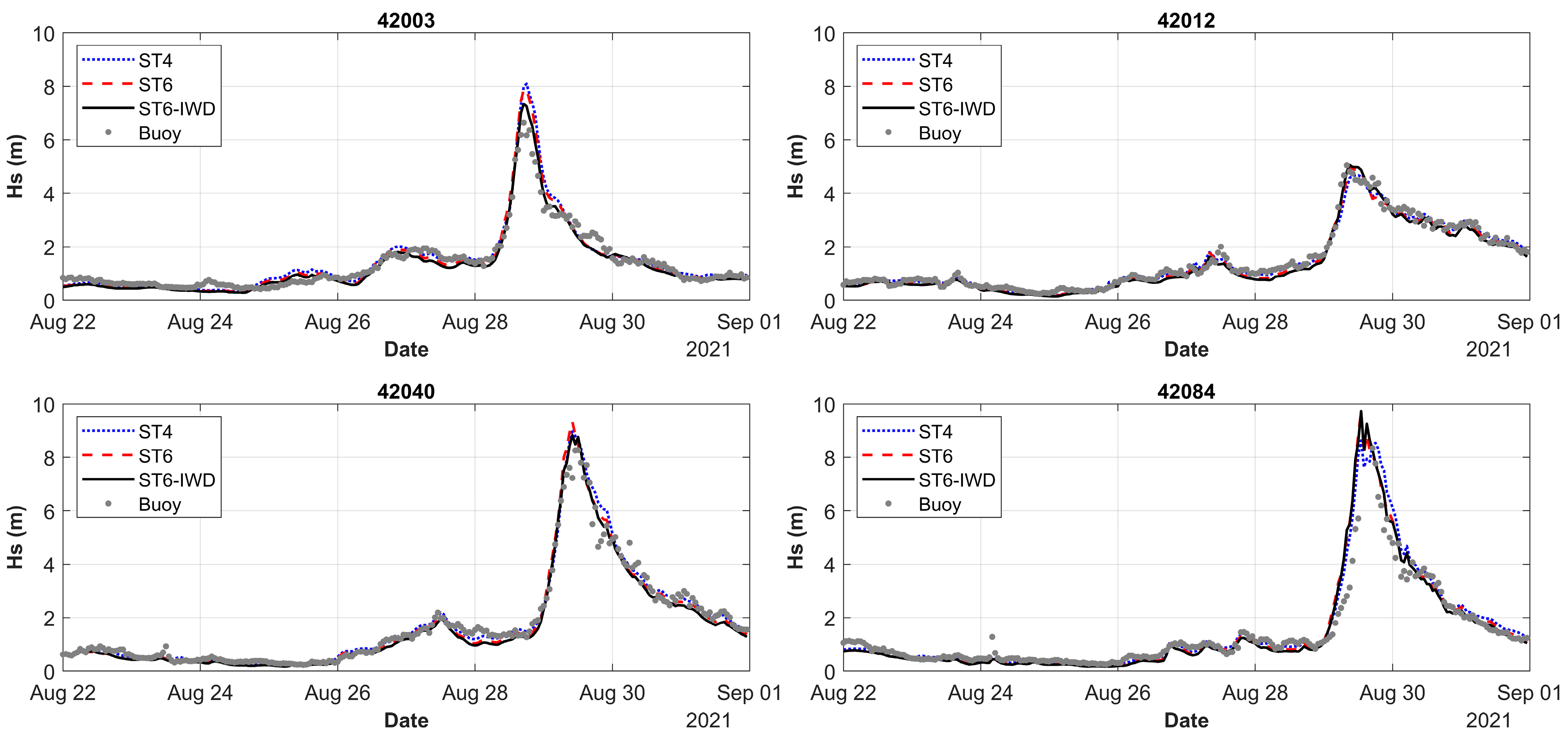
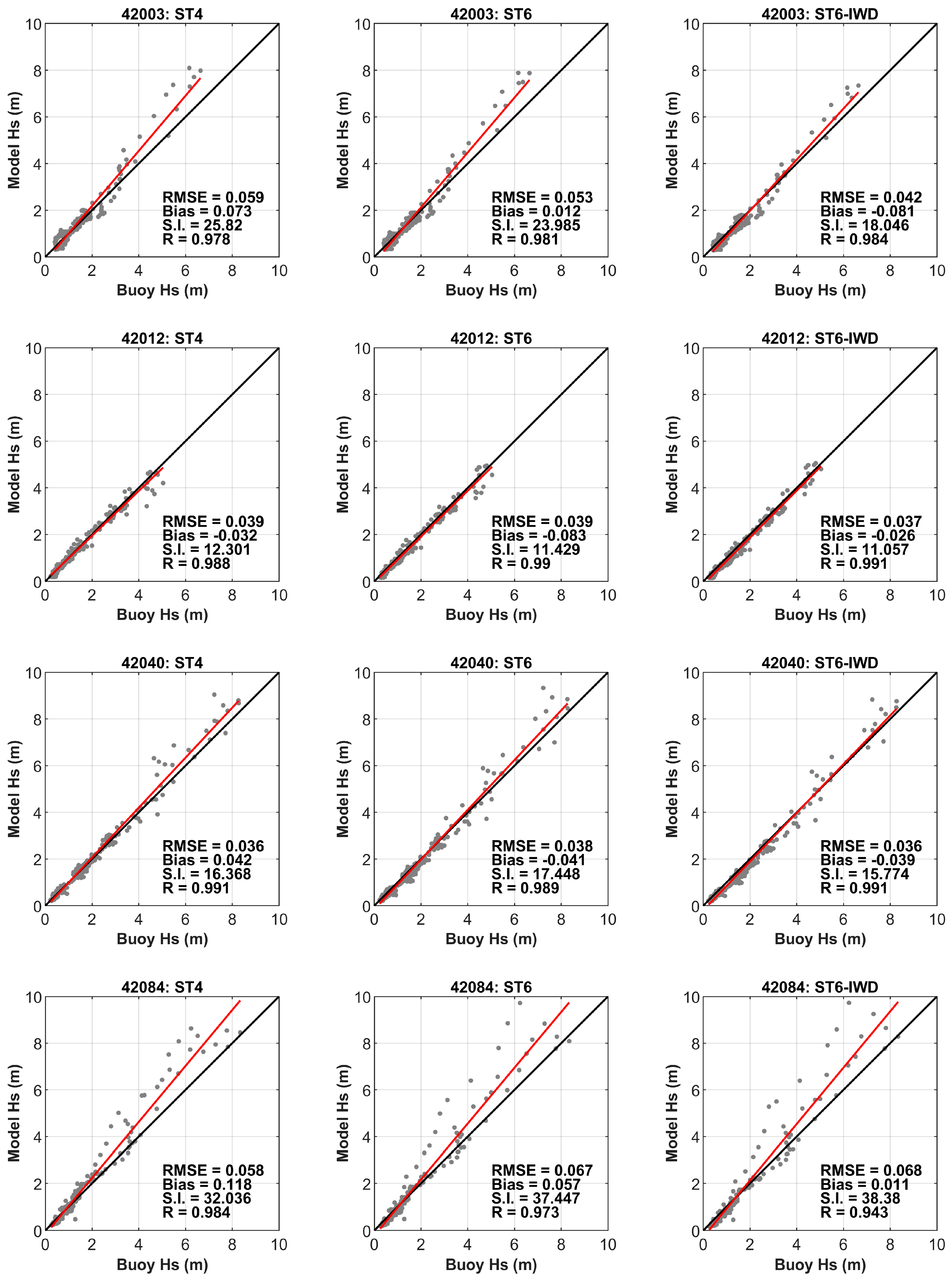
• The significant wave heights computed for cases ST4, ST6, and ST6-IWD were compared with in situ observations. It was noticed that the standard ST4 scheme did not perform well under hurricane wind conditions and tended to underestimate the peak wave heights generated by Hurricane Ida, while the ST6 and ST6-IWD schemes performed well for extreme wind conditions. The percentage error ranges computed for all three cases were as follows: ST4: −4.47% to 15.71%, ST6: −1% to 14.29%, and ST6-IWD: 0.97% to 10% (negative % indicates underestimation and positive % indicates overestimation). From the error range metrics and statistical indicators, it can be seen that the ST6-IWD method performed better than ST4 and ST6 in terms of peak wave height estimation. The main advantage of ST6-IWD over ST6 is that the wind input source term requires a cut-off function only beyond ~113 m/s, whereas the latter needs it after 50 m/s wind speeds.
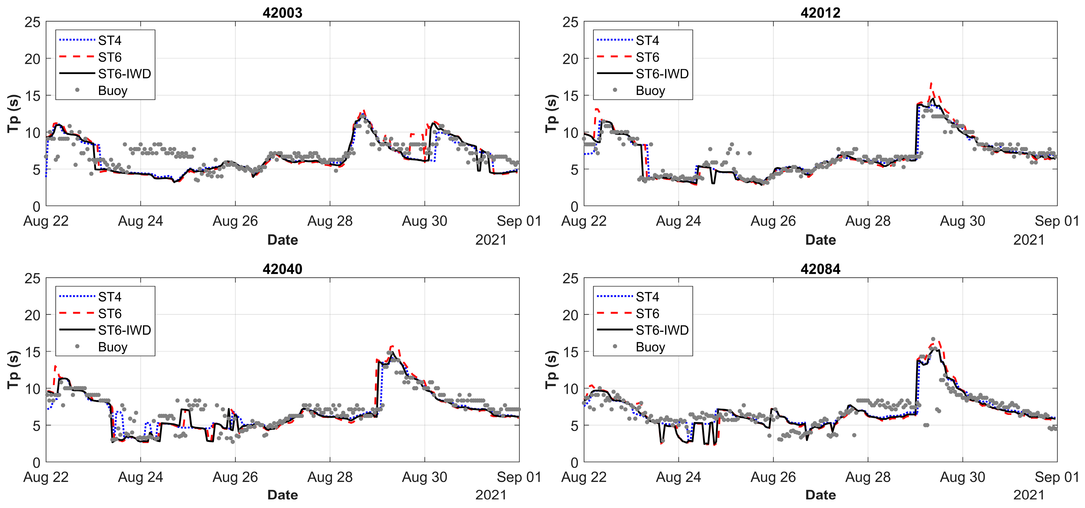
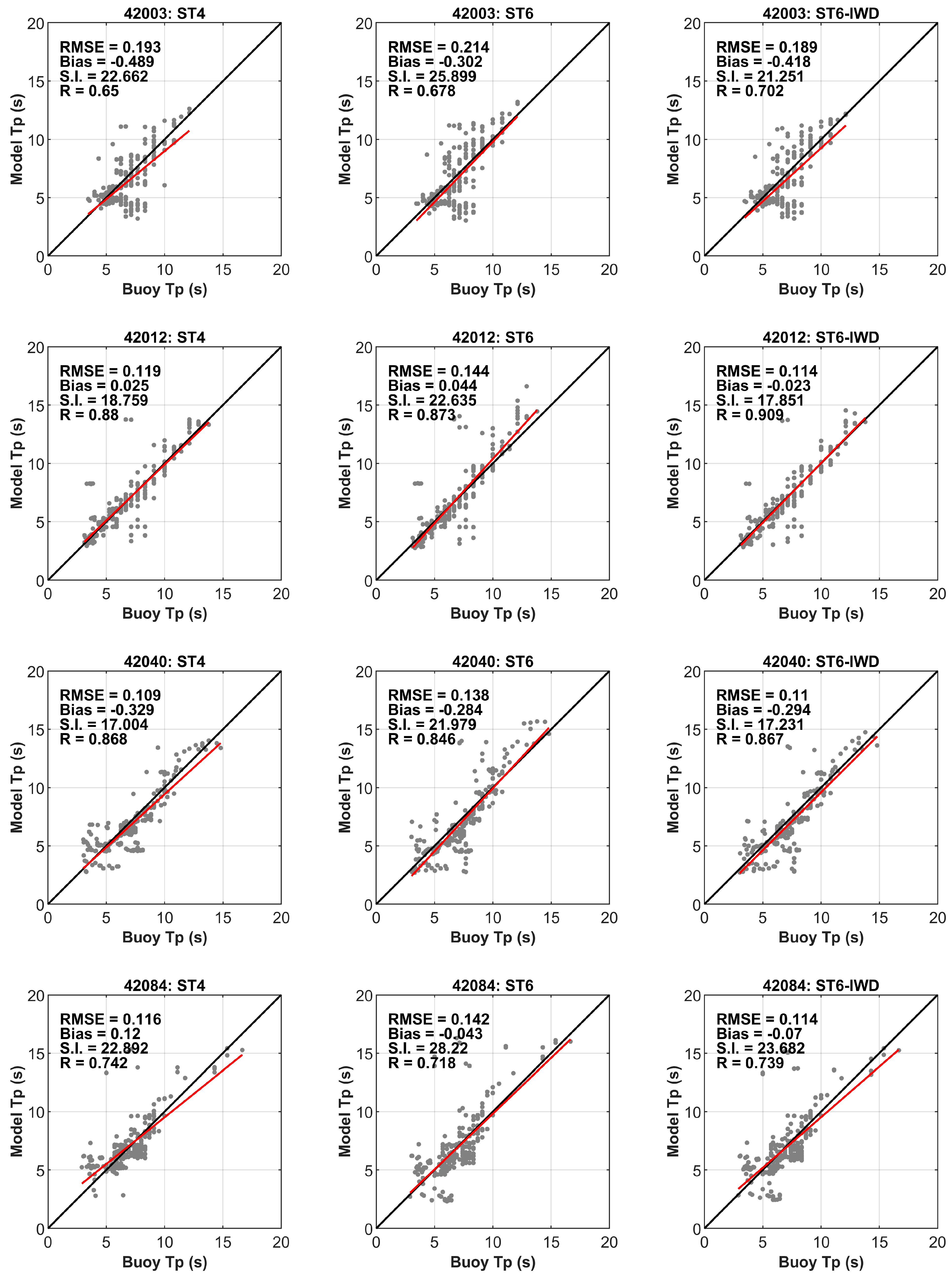
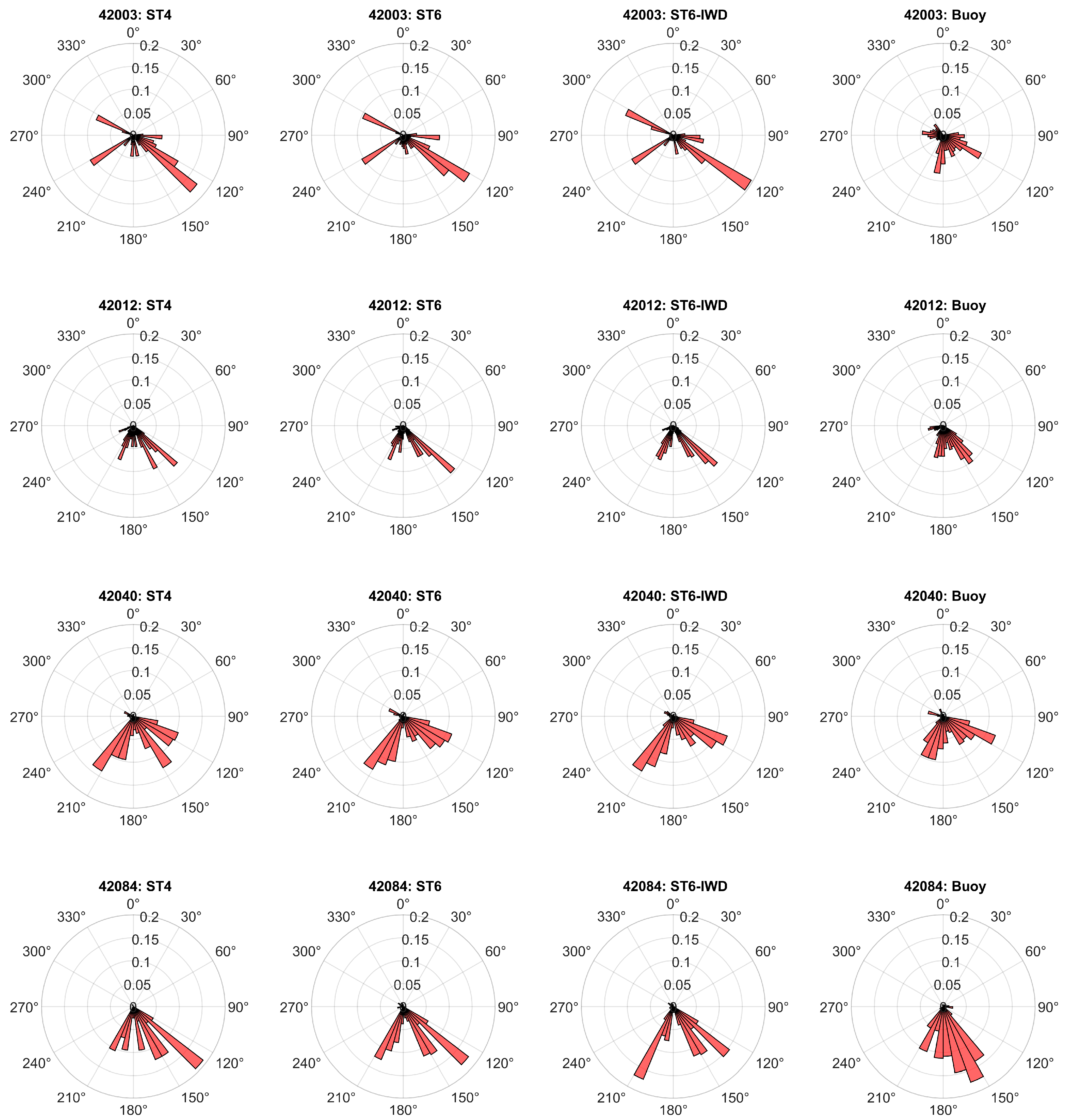
• The peak wave periods and peak wave directions also emphasized that the ST6-IWD-based estimations were better than the those of the ST4 and ST6 schemes. This was further confirmed through statistical estimates, where ST6 had the highest RMSE compared to ST6-IWD and ST4. Therefore, it is imperative to recommend the ST6-IWD scheme for performing storm wave simulations for the Gulf of Mexico basin. The improved accuracy of the ST6-IWD scheme in capturing peak wave characteristics makes it a valuable tool for predicting storm impacts. Additionally, its ability to handle higher wind speeds without requiring a cut-off function further enhances its reliability for extreme weather conditions.
• Further study is required to conduct a comprehensive analysis of how these schemes perform with different configurations of unstructured grids. Additionally, it is important to investigate how these schemes respond to other hurricanes in the Gulf and cyclones that evolve in various other regions, such as in the northern Indian Ocean and the western Pacific Ocean. This broader analysis will help validate the robustness and adaptability of the ST6-IWD scheme (in WW3) across diverse meteorological conditions and geographical locations.

References

1. Beven, J.L.; Hagen, A.; Berg, R. National Hurricane Center Tropical Cyclone Report; NOAA: Silver Spring, MD, USA, 2022; pp. 1–163. [Google Scholar]
2. NOAA-NCEI. U.S. Billion-Dollar Weather and Climate Disasters. 2024. Available online: https://www.ncei.noaa.gov/access/billions/ (accessed on 14 December 2024).
3. Janssen, P.A.; Viterbo, P. Ocean waves and the atmospheric climate. J. Clim. 1996, 9, 1269–1287. [Google Scholar] [CrossRef]
4. Janssen, P.A.E.M.; Doyle, J.D.; Bidlot, J.; Hansen, B.; Isaksen, L.; Viterbo, P. Impact and feedback of ocean waves on the atmosphere. Adv. Fluid Mech. 2002, 33, 155–198. [Google Scholar]
5. Wahle, K.; Staneva, J.; Koch, W.; Fenoglio-Marc, L.; Ho-Hagemann, H.; Stanev, E.V. An atmosphere–wave regional coupled model: Improving predictions of wave heights and surface winds in the southern North Sea. Ocean Sci. 2017, 13, 289–301. [Google Scholar] [CrossRef]
6. Shankar, C.G.; Cambazoglu, M.K.; Bernstein, D.N.; Hesser, T.J.; Wiggert, J.D. Sensitivity and impact of atmospheric forcings on hurricane wind wave modeling in the Gulf of Mexico using nested WAVEWATCH III. Appl. Ocean Res. 2025, 154, 104320. [Google Scholar] [CrossRef]
7. Valiente, N.G.; Saulter, A.; Edwards, J.M.; Lewis, H.W.; Castillo Sanchez, J.M.; Bruciaferri, D.; Bunney, C.; Siddorn, J. The impact of wave model source terms and coupling strategies to rapidly developing waves across the north-west european shelf during extreme events. J. Mar. Sci. Eng. 2021, 9, 403. [Google Scholar] [CrossRef]
8. Shankar, C.G.; Behera, M.R. Wave Boundary Layer Model based wind drag estimation for tropical storm surge modelling in the Bay of Bengal. Ocean Eng. 2019, 191, 106509. [Google Scholar] [CrossRef]
9. Shankar, C.G.; Behera, M.R. Improved wind drag formulation for numerical storm wave and surge modeling. Dyn. Atmos. Ocean. 2021, 93, 101193. [Google Scholar] [CrossRef]
10. Charnock, H. Wind stress on a water surface. Q. J. R. Meteorol. Soc. 1955, 81, 639–640. [Google Scholar] [CrossRef]
11. Smith, S.D.; Banke, E.G. Variation of the sea surface drag coefficient with wind speed. Q. J. R. Meteorol. Soc. 1975, 101, 665–673. [Google Scholar] [CrossRef]
12. Garratt, J.R. Review of drag coefficients over oceans and continents. Mon. Weather. Rev. 1977, 105, 915–929. [Google Scholar] [CrossRef]
13. Large, W.G.; Pond, S. Open ocean momentum flux measurements in moderate to strong winds. J. Phys. Oceanogr. 1981, 11, 324–336. [Google Scholar] [CrossRef]
14. Wu, J. Wind-stress coefficients over sea surface from breeze to hurricane. J. Geophys. Res. Ocean. 1982, 87, 9704–9706. [Google Scholar] [CrossRef]
15. Guan, C.; Xie, L. On the linear parameterization of drag coefficient over sea surface. J. Phys. Oceanogr. 2004, 34, 2847–2851. [Google Scholar] [CrossRef]
16. Gao, Z.; Wang, Q.; Wang, S. An alternative approach to sea surface aerodynamic roughness. J. Geophys. Res. Atmos. 2006, 111, D22108. [Google Scholar] [CrossRef]
17. Powell, M.D.; Vickery, P.J.; Reinhold, T.A. Reduced drag coefficient for high wind speeds in tropical cyclones. Nature 2003, 422, 279–283. [Google Scholar] [CrossRef]
18. Donelan, M.A.; Haus, B.K.; Reul, N.; Plant, W.J.; Stiassnie, M.; Graber, H.C.; Brown, O.B.; Saltzman, E.S. On the limiting aerodynamic roughness of the ocean in very strong winds. Geophys. Res. Lett. 2004, 31, L18306. [Google Scholar] [CrossRef]
19. Jarosz, E.; Mitchell, D.A.; Wang, D.W.; Teague, W.J. Bottom-up determination of air-sea momentum exchange under a major tropical cyclone. Science 2007, 315, 1707–1709. [Google Scholar] [CrossRef]
20. Hwang, P.A. A note on the ocean surface roughness spectrum. J. Atmos. Ocean. Technol. 2011, 28, 436–443. [Google Scholar] [CrossRef]
21. Holthuijsen, L.H.; Powell, M.D.; Pietrzak, J.D. Wind and waves in extreme hurricanes. J. Geophys. Res. Ocean. 2012, 117, C09003. [Google Scholar] [CrossRef]
22. Zijlema, M.; Van Vledder, G.P.; Holthuijsen, L.H. Bottom friction and wind drag for wave models. Coast. Eng. 2012, 65, 19–26. [Google Scholar] [CrossRef]
23. Makin, V.K.; Kudryavtsev, V.N. Coupled sea surface-atmosphere model: 1. Wind over waves coupling. J. Geophys. Res. Ocean. 1999, 104, 7613–7623. [Google Scholar] [CrossRef]
24. Makin, V.K.; Kudryavtsev, V.N. Impact of dominant waves on sea drag. Bound.-Layer Meteorol. 2002, 103, 83–99. [Google Scholar] [CrossRef]
25. Hara, T.; Belcher, S.E. Wind forcing in the equilibrium range of wind-wave spectra. J. Fluid Mech. 2002, 470, 223–245. [Google Scholar] [CrossRef]
26. Hara, T.; Belcher, S.E. Wind profile and drag coefficient over mature ocean surface wave spectra. J. Phys. Oceanogr. 2004, 34, 2345–2358. [Google Scholar] [CrossRef]
27. Moon, I.J.; Hara, T.; Ginis, I.; Belcher, S.E.; Tolman, H.L. Effect of surface waves on air–sea momentum exchange. Part I: Effect of mature and growing seas. J. Atmos. Sci. 2004, 61, 2321–2333. [Google Scholar] [CrossRef]
28. Du, J.; Larsén, X.G.; Chen, S.; Bolaños, R.; Badger, M.; Yang, Y. The impact of wind–wave coupling with WBLM on coastal storm simulations. Ocean Model. 2022, 180, 102135. [Google Scholar] [CrossRef]
29. Janssen, P.A.; Bidlot, J.R. Wind–wave interaction for strong winds. J. Phys. Oceanogr. 2023, 53, 779–804. [Google Scholar] [CrossRef]
30. Makrygianni, N.; Pan, S.; Bray, M.; Bidlot, J.R. Modelling of hurricane Dorian via the implementation of Wave Boundary Layer Model (WBLM) within the OpenIFS. Ocean Model. 2025, 194, 102469. [Google Scholar] [CrossRef]
31. Moon, I.J.; Ginis, I.; Hara, T.; Thomas, B. A physics-based parameterization of air–sea momentum flux at high wind speeds and its impact on hurricane intensity predictions. Mon. Weather Rev. 2007, 135, 2869–2878. [Google Scholar] [CrossRef]
32. Reichl, B.G.; Hara, T.; Ginis, I. Sea state dependence of the wind stress over the ocean under hurricane winds. J. Geophys. Res. Ocean. 2014, 119, 30–51. [Google Scholar] [CrossRef]
33. Zhao, B.; Wu, L.; Wang, G.; Zhang, J.A.; Liu, L.; Zhao, C.; Zhuang, Z.; Xia, C.; Xue, Y.; Li, X.; et al. A numerical study of tropical cyclone and ocean responses to air-sea momentum flux at high winds. J. Geophys. Res. Ocean. 2024, 129, e2024JC020956. [Google Scholar] [CrossRef]
34. Chen, Y.; Yu, X. Enhancement of wind stress evaluation method under storm conditions. Clim. Dyn. 2016, 47, 3833–3843. [Google Scholar] [CrossRef]
35. Chen, Y.; Yu, X. Sensitivity of storm wave modeling to wind stress evaluation methods. J. Adv. Model. Earth Syst. 2017, 9, 893–907. [Google Scholar] [CrossRef]
36. Shankar, C.G.; Behera, M.R. Numerical analysis on the effect of wave boundary condition in storm wave and surge modeling for a tropical cyclonic condition. Ocean Eng. 2021, 220, 108371. [Google Scholar] [CrossRef]
37. Luettich, R.A.; Westerink, J.J.; Scheffner, N.W. ADCIRC: An Advanced Three-Dimensional Circulation Model for Shelves, Coasts, and Estuaries. Report 1. Theory and Methodology of ADCIRC-2DDI and ADCIRC-3DL. 1992. [Google Scholar]
38. Booij, N.R.R.C.; Ris, R.C.; Holthuijsen, L.H. A third-generation wave model for coastal regions: 1. Model description and validation. J. Geophys. Res. Ocean. 1999, 104, 7649–7666. [Google Scholar] [CrossRef]
39. Tolman, H.L.; Chalikov, D. Source terms in a third-generation wind wave model. J. Phys. Oceanogr. 1996, 26, 2497–2518. [Google Scholar] [CrossRef]
40. Hasselmann, K. On the spectral dissipation of ocean waves due to white capping. Bound.-Layer Meteorol. 1974, 6, 107–127. [Google Scholar] [CrossRef]
41. Snyder, R.L.; Dobson, F.W.; Elliott, J.A.; Long, R.B. Array measurements of atmospheric pressure fluctuations above surface gravity waves. J. Fluid Mech. 1981, 102, 1–59. [Google Scholar] [CrossRef]
42. Komen, G.J.; Hasselmann, S.; Hasselmann, K. On the existence of a fully developed wind-sea spectrum. J. Phys. Oceanogr. 1984, 14, 1271–1285. [Google Scholar] [CrossRef]
43. Chalikov, D.V.; Belevich, M.Y. One-dimensional theory of the wave boundary layer. Bound.-Layer Meteorol. 1993, 63, 65–96. [Google Scholar] [CrossRef]
44. Chalikov, D. The parameterization of the wave boundary layer. J. Phys. Oceanogr. 1995, 25, 1333–1349. [Google Scholar] [CrossRef]
45. Janssen, P. The Interaction of Ocean Waves and Wind; Cambridge University Press: Cambridge, UK, 2004. [Google Scholar]
46. Bidlot, J.R.; Abdalla, S.; Janssen, P. A Revised Formulation for Ocean Wave Dissipation in cy25r1; Research Department, ECMWF: Reading, UK, 2005. [Google Scholar]
47. Ardhuin, F.; Rogers, E.; Babanin, A.V.; Filipot, J.F.; Magne, R.; Roland, A.; Van Der Westhuysen, A.; Queffeulou, P.; Lefevre, J.M.; Aouf, L.; et al. Semiempirical dissipation source functions for ocean waves. Part I: Definition, calibration, and validation. J. Phys. Oceanogr. 2010, 40, 1917–1941. [Google Scholar] [CrossRef]
48. Zieger, S.; Babanin, A.V.; Rogers, W.E.; Young, I.R. Observation-based source terms in the third-generation wave model WAVEWATCH. Ocean Model. 2015, 96, 2–25. [Google Scholar] [CrossRef]
49. Liu, Q.; Rogers, W.E.; Babanin, A.V.; Young, I.R.; Romero, L.; Zieger, S.; Qiao, F.; Guan, C. Observation-based source terms in the third-generation wave model WAVEWATCH III: Updates and verification. J. Phys. Oceanogr. 2019, 49, 489–517. [Google Scholar] [CrossRef]
50. Umesh, P.A.; Behera, M.R. Performance evaluation of input-dissipation parameterizations in WAVEWATCH III and comparison of wave hindcast with nested WAVEWATCH III-SWAN in the Indian Seas. Ocean Eng. 2020, 202, 106959. [Google Scholar] [CrossRef]
51. van Vledder, G.P.; Hulst, S.T.C.; McConochie, J.D. Source term balance in a severe storm in the Southern North Sea. Ocean Dyn. 2016, 66, 1681–1697. [Google Scholar] [CrossRef]
52. Christakos, K.; Furevik, B.R.; Aarnes, O.J.; Breivik, Ø.; Tuomi, L.; Byrkjedal, Ø. The importance of wind forcing in fjord wave modelling. Ocean Dyn. 2020, 70, 57–75. [Google Scholar] [CrossRef]
53. Christakos, K.; Björkqvist, J.V.; Tuomi, L.; Furevik, B.R.; Breivik, Ø. Modelling wave growth in narrow fetch geometries: The white-capping and wind input formulations. Ocean Model. 2021, 157, 101730. [Google Scholar] [CrossRef]
54. NOAA-NCEI. Monthly National Climate Report for July 2021, Published Online August 2021. 2021. Available online: https://www.ncei.noaa.gov/access/monitoring/monthly-report/national/202107 (accessed on 14 December 2024).
55. Benjamin, S.G.; Dévényi, D.; Weygandt, S.S.; Brundage, K.J.; Brown, J.M.; Grell, G.A.; Kim, D.; Schwartz, B.E.; Smirnova, T.G.; Smith, T.L.; et al. An hourly assimilation–forecast cycle: The RUC. Mon. Weather Rev. 2004, 132, 495–518. [Google Scholar] [CrossRef]
56. Smith, T.L.; Benjamin, S.G.; Gutman, S.I.; Sahm, S. Short-range forecast impact from assimilation of GPS-IPW observations into the Rapid Update Cycle. Mon. Weather Rev. 2007, 135, 2914–2930. [Google Scholar] [CrossRef]
57. Benjamin, S.G.; Weygandt, S.S.; Brown, J.M.; Hu, M.; Alexander, C.R.; Smirnova, T.G.; Olson, J.B.; James, E.P.; Dowell, D.C.; Grell, G.A.; et al. A North American hourly assimilation and model forecast cycle: The Rapid Refresh. Mon. Weather Rev. 2016, 144, 1669–1694. [Google Scholar] [CrossRef]
58. Dowell, D.C.; Alexander, C.R.; James, E.P.; Weygandt, S.S.; Benjamin, S.G.; Manikin, G.S.; Blake, B.T.; Brown, J.M.; Olson, J.B.; Hu, M.; et al. The High-Resolution Rapid Refresh (HRRR): An hourly updating convection-allowing forecast model. Part I: Motivation and system description. Weather Forecast. 2022, 37, 1371–1395. [Google Scholar] [CrossRef]
59. James, E.P.; Alexander, C.R.; Dowell, D.C.; Weygandt, S.S.; Benjamin, S.G.; Manikin, G.S.; Brown, J.M.; Olson, J.B.; Hu, M.; Smirnova, T.G.; et al. The High-Resolution Rapid Refresh (HRRR): An hourly updating convection-allowing forecast model. Part II: Forecast Performance. Weather Forecast. 2022, 37, 1397–1417. [Google Scholar]
60. Haiden, T.; Janousek, M.; Bidlot, J.; Ferranti, L.; Prates, F.; Vitart, F.; Bauer, P.; Richardson, D.S. Evaluation of ECMWF Forecasts, Including the 2016 Resolution Upgrade; European Centre for Medium Range Weather Forecasts: Reading, UK, 2016. [Google Scholar]
61. Yang, D.; Wang, W.; Bright, J.M.; Voyant, C.; Notton, G.; Zhang, G.; Lyu, C. Verifying operational intra-day solar forecasts from ECMWF and NOAA. Sol. Energy 2022, 236, 743–755. [Google Scholar] [CrossRef]
62. Chawla, A.; Tolman, H.L. Automated grid generation for WAVEWATCH III. Tech. Bull. 2007, 254, 277. [Google Scholar]
63. Chawla, A.; Tolman, H.L. Obstruction grids for spectral wave models. Ocean Model. 2008, 22, 12–25. [Google Scholar] [CrossRef]
64. Hasselmann, K.; Barnett, T.P.; Bouws, E.; Carlson, H.; Cartwright, D.E.; Enke, K.; Ewing, J.A.; Gienapp, A.; Hasselmann, D.E.; Kruseman, P.; et al. Measurements of wind-wave growth and swell decay during the Joint North Sea Wave Project (JONSWAP). Ergaenzungsheft zur Deutschen Hydrographischen Zeitschrift, Reihe A. 1973. [Google Scholar]
65. Hasselmann, D.E.; Dunckel, M.; Ewing, J.A. Directional wave spectra observed during JONSWAP 1973. J. Phys. Oceanogr. 1980, 10, 1264–1280. [Google Scholar] [CrossRef]
66. Hersbach, H.; Bell, B.; Berrisford, P.; Biavati, G.; Horányi, A.; Muñoz Sabater, J.; Nicolas, J.; Peubey, C.; Radu, R.; Rozum, I.; et al. ERA5 Hourly Data on Single Levels from 1940 to Present. Copernicus Climate Change Service (C3S) Climate Data Store (CDS). 2023. Available online: https://cds.climate.copernicus.eu/datasets/reanalysis-era5-single-levels?tab=overview (accessed on 11 January 2024).
67. The WAVEWATCH III R Development Group (WW3DG). User Manual and System Documentation of WAVEWATCH III R Version 6.07; Tech. Note 333; NOAA/NWS/NCEP/MMAB: College Park, MD, USA, 2019; 465p.
Figure 1. Nested multi-grid with variable resolutions for WAVEWATCH III model domain along with its water depth (m) adopted in this study. The resolutions set for the model grids are as follows: GOM (0.15° resolution, blue dash box); N1 (0.05° resolution, brown dash box); N2 (0.02° resolution, black dash box). NDBC stations 42003, 42012, 42040, 42084, and BURL1 where the model results were compared with observations are also demarcated.
Jmse 13 00403 g001
Figure 2. Hurricane Ida’s wind speed (m/s) time series comparison between model (HRRR) and buoy (42003, 42012, and 42040)/C-MAN (BURL1) stations.
Jmse 13 00403 g002
Figure 3. HRRR wind speeds (m/s) compared with observations at NDBC buoys (42003, 42012, and 42040) and C-MAN station (BURL1) during Hurricane Ida along with their statistical error estimates for RMSE, bias, SI (%) and R. The black lines show the 1:1 ratio, and the red lines show the best fits.
Jmse 13 00403 g003
Figure 4. Hurricane Ida’s track, wind speed (m/s), and the corresponding wind drag coefficient (Cd—contours labeled in yellow) computed by each of the methods (ST4, ST6, and ST6-IWD) on 29 August 2021 at 1200 UTC.
Jmse 13 00403 g004
Figure 5. (Top) Maximum wind speed (m/s) of Hurricane Ida from HRRR, with the approximate location (yellow) where the maximum winds were observed. (Bottom) Comparison of the wind drag coefficient (Cd) as a function of wind speed between the ST4, ST6, and ST6-IWD methods at the approximate location of the maximum winds.
Jmse 13 00403 g005
Figure 6. Hurricane Ida’s significant wave height (m) time series comparison between model (ST4, ST6, and ST6-IWD) and buoy (42003, 42012, 42040, and 42084) locations.
Jmse 13 00403 g006
Figure 7. Model results (ST4, ST6, and ST6-IWD) for significant wave heights (m) compared with observations at NDBC buoys (42003, 42012, 42040, and 42084) during Hurricane Ida along with their statistical error estimates for RMSE, bias, SI(%), and R. The black lines show the 1:1 ratio, and the red lines show the best fits.
Jmse 13 00403 g007
Figure 8. Hurricane Ida’s track and significant wave height (m) distribution along with its contours on 29 August 2021 at 1200 UTC spatially covering the N1 grid of the wave model for all three cases, ST4, ST6, and ST6-IWD.
Jmse 13 00403 g008
Figure 9. Hurricane Ida’s peak wave period (s) time series comparison between model (ST4, ST6, and ST6-IWD) and buoy (42003, 42012, 42040, and 42084) locations.
Jmse 13 00403 g009
Figure 10. Model results (ST4, ST6, and ST6-IWD) for peak wave periods (m) compared with observations at NDBC buoys (42003, 42012, 42040, and 42084) during Hurricane Ida along with their statistical error estimates for RMSE, bias, SI(%), and R. The black lines show the 1:1 ratio, and the red lines show the best fits.
Jmse 13 00403 g010
Figure 11. Hurricane Ida’s peak wave direction (deg) comparison between model (ST4, ST6, and ST6-IWD) and buoy (42003, 42012, 42040, and 42084) locations.
Jmse 13 00403 g011
Disclaimer/Publisher’s Note: The statements, opinions and data contained in all publications are solely those of the individual author(s) and contributor(s) and not of MDPI and/or the editor(s). MDPI and/or the editor(s) disclaim responsibility for any injury to people or property resulting from any ideas, methods, instructions or products referred to in the content.