Investigating Morison Modeling of Viscous Forces by Steep Waves on Columns of a Fixed Floating Offshore Wind Turbine (FOWT) Using Computational Fluid Dynamics (CFD)

Abstract

Mean and slowly varying wave loads on floating offshore wind turbines (FOWTs) need to be estimated accurately for the design of mooring systems. The low-frequency drift forces are underestimated by potential flow theory, especially in steep waves. Viscous forces on columns is an important contributor which could be included by adding the quadratic drag of Morison formulation to the potential flow solution. The drag coefficients in Morison equation can be determined based on an empirical formula, CFD study, or model testing. In the WINDMOOR project, a FOWT support structure, composed of three columns joined at the bottom by pontoons and at the top by deck beams, is studied using CFD. In order to extract the KC-dependent drag coefficients, a series of simulations for the fixed structure in regular waves is performed with the CFD code STAR-CCM+. In this study, the forces along each column of the FOWT are analyzed using the results of CFD as well as potential flow simulations. The hydrodynamic interactions between the columns are addressed. A methodology is proposed to process the CFD results of forces on the columns and extract the contribution of viscous effects. Limitations of the Morison drag model to represent extracted viscous forces in steep waves are investigated. The obtained drag coefficients are compared with the available data in the literature. It is shown that accounting for potential flow interactions and nonlinear flow kinematics could, to a large degree, explain the previously reported differences between drag coefficients for a column in waves. Moreover, it is shown that the proposed model can capture the contribution of viscous effects to mean drift forces for fixed columns in waves.

1. Introduction

Mean and slowly varying wave loads and motions are important for the designing of mooring systems for floating offshore structures. Column-based offshore wind turbines are no exception. Linear potential flow solvers such as WAMIT are often used to determining the mean drift force coefficients. It is well known that this method under-predicts the drift loads, especially in the low-frequency range relevant for resonant slowly varying motions of moored structures (see, for example, [1]). This under-prediction is mainly attributed to viscous forces, which are neglected in the potential flow solution of drift forces. Wang et al. [2] studied the responses of a FOWT in waves experimentally and reported that low-frequency motions are consistently under-predicted by the available mid-fidelity engineering tools. They attribute this effect to the under-prediction of viscous drag forces on columns.

The Morison force model, shown in Equation (1), is a well-established model for considering viscous forces on columns. In this model, the total force on a column is decomposed to inertia and drag components:

$$F={\displaystyle \frac{1}{2}}\rho D{C}_D{u}_r\left|u_r\right|+\rho \pi {\displaystyle \frac{D^2}{4}}{C}_M\dot{u}$$

(1)

Here, $u_r$ is the relative fluid velocity between the body and fluid, and $\dot{u}$ is the fluid’s acceleration. $\rho$ and D represent the fluid density and the column’s diameter, respectively. $C_D$ and $C_M$ are usually refereed to as the drag and mass coefficients. It has been shown that when the wave length is roughly more than five times the column’s diameter, known as the long wave condition, this model gives a good representation of forces (see, for example, [3] among others). For shorter waves, radiation and diffraction effects must be considered in estimating forces.

The Morison model of forces is widely used in state-of-the-art time-domain simulation tools for the motions of offshore structures (e.g., SIMO [4]). Usually, a constant drag and mass coefficients are selected based on empirical, numerical, or model testing to represent the forces in these programs. For a fixed structure in waves, the wave particle velocities are often simplified to a pure harmonic oscillatory motions. The mass and drag coefficients of an oscillating column’s cross section in the absence of a current depend on several factors such as the following:

• Keulegan–Carpenter number ($KC=u_{m}T/D=2\pi {\eta }_a/D$), where $u_m$ is the maximum relative velocity between the body and fluid, and T and ${\eta }_a$ are the oscillation period and amplitude, respectively.
• Reynolds number: $Rn=u_{m}D/\nu =2\pi {\eta }_{a}D/\left(\nu T\right)$, where $\nu$ is kinematic viscosity, or $\beta =Rn/KC=D^2/\left(\nu T\right)$.
• Roughness number, $k/D$, where k is the characteristic roughness size.

The influence of $KC$, $\beta$, and surface roughness on the coefficients has been studied extensively in the past.

Table 1. Previous studies focusing on mass and drag coefficients of a circular cylinder in pure oscillatory flow.

Article	$\mathbf{KC}$-Range	$\mathit{\beta }$-Range	$\mathit{k}/\mathit{D}$
Sarpkaya (1977) [6]	2–100	497–5260	smooth, 1/100, 1/800
Bearman et al. (1985) [7]	0.2–10	196–1665	smooth
Sarpkaya (1986) [8]	0.4–25	1035–11,240	smooth-1/100
Chaplin (1988) [9]	4–20	2000–28,000	smooth
Justesen (1988) [10]	1–20	${10}^4$–${10}^5$	smooth, 1/50
Anaturk (1991) [11]	0.1–10	29,000–136,000	smooth-1/50
Troesch and Kim (1991) [12]	0.1–1.0	23,200–48,600	smooth
Bearman and Mackwood (1992) [13]	0.1–3.0	<$3\times {10}^4$	smooth, 1/50
Chaplin (1993) [14]	5–25	${10}^4$–${10}^5$	$1.{210}^{-4}$
Gao et al. (2020) [15]	0.04–5.0	20,950	smooth

includes an incomplete list of such studies, together with the considered ranges of the parameters. The strong dependency of both mass and drag coefficients on the KC number is reported for the considered range of values. In practice, empirical formulas, such as the one presented in the Recommended Practice by DNV [5], is usually adopted to estimate drag and mass coefficients.

In addition to the above-mentioned parameters, the following effects are not directly considered in the Morison force model, and when important, they are usually considered by varying mass and drag coefficients:

• Free-surface effects;
• Truncation, 3D effects;
• Interactions between columns;
• Non-planar velocities due to waves.

The importance of truncation effects is investigated by Nakamura et al. [16] by studying the effects of the aspect ratio on the drag and mass forces of a circular cylinder with $KC$ values between 4 and 40. They show that not only does the drag coefficient change with the aspect ratio but the $KC$ dependency of the drag forces changes as well. Meaning, especially at lower $KC$ values, the effect of increasing the aspect ratio could be different compared to high $KC$ values. Vengatesan et al. [17] studies forces on a truncated rectangular cylinder due to regular and random waves, and reports similar findings about the effect of the aspect ratio.

Computational Fluid Dynamics (CFD) is a good candidate for studying wave forces on columns when considering a combination of the above effects in a realistic condition. An important example of CFD application in studying wave loads on a bottom-mounted circular is the work by Paulsen et al. [18], which investigates secondary load cycle in presence of steep waves. More recently, Clément et al. [19] have studied the force on a restrained cylinder in a regular wave using CFD. In their study, the forces calculated by CFD are decomposed to Morison coefficients for different sections along the cylinder, and the applicability range of the Morison load model is evaluated. Wang et al. [20] investigates the application of CFD in estimating difference-frequency wave loads and show that it is possible to capture viscous effects on drift forces to improve the engineering prediction of slowly varying motions.

A fixed column-based structure in waves, without current, is considered in the present study, focusing on viscous forces on columns and their contribution to mean drift forces. CFD is often used to quantify viscous and other nonlinear forces on columns in waves. However, in order to effectively use the findings in time-domain simulations, the forces obtained from CFD are used to extract drag coefficients for Morison-type force models. This has proven to be challenging due to the presence of nonlinear flow kinematics, diffracted waves, and proximity to the free surface.

In the present study, a methodology for extracting sectional drag coefficients from the CFD results of a fixed FOWT in a series of regular waves is investigated. In this method, linear forces are estimated using potential flow theory and subtracted from the CFD forces. Further, a quadratic Morison drag model is fitted to the remaining force, and a mean drag coefficient is extracted, while nonlinear flow kinematics and free surface approximately are considered. A description of selected wave conditions, and the CFD setup is given Section 2, followed by the processing method for calculating residual forces, fitting Morison drag models, and extracting drag coefficients. Section 3 presents the CFD results and the obtained drag coefficients by using different assumptions for wave kinematics. Furthermore, the ability of the obtained model in representing wave frequency and mean drift forces is investigated by comparing the calculated forces with CFD results.

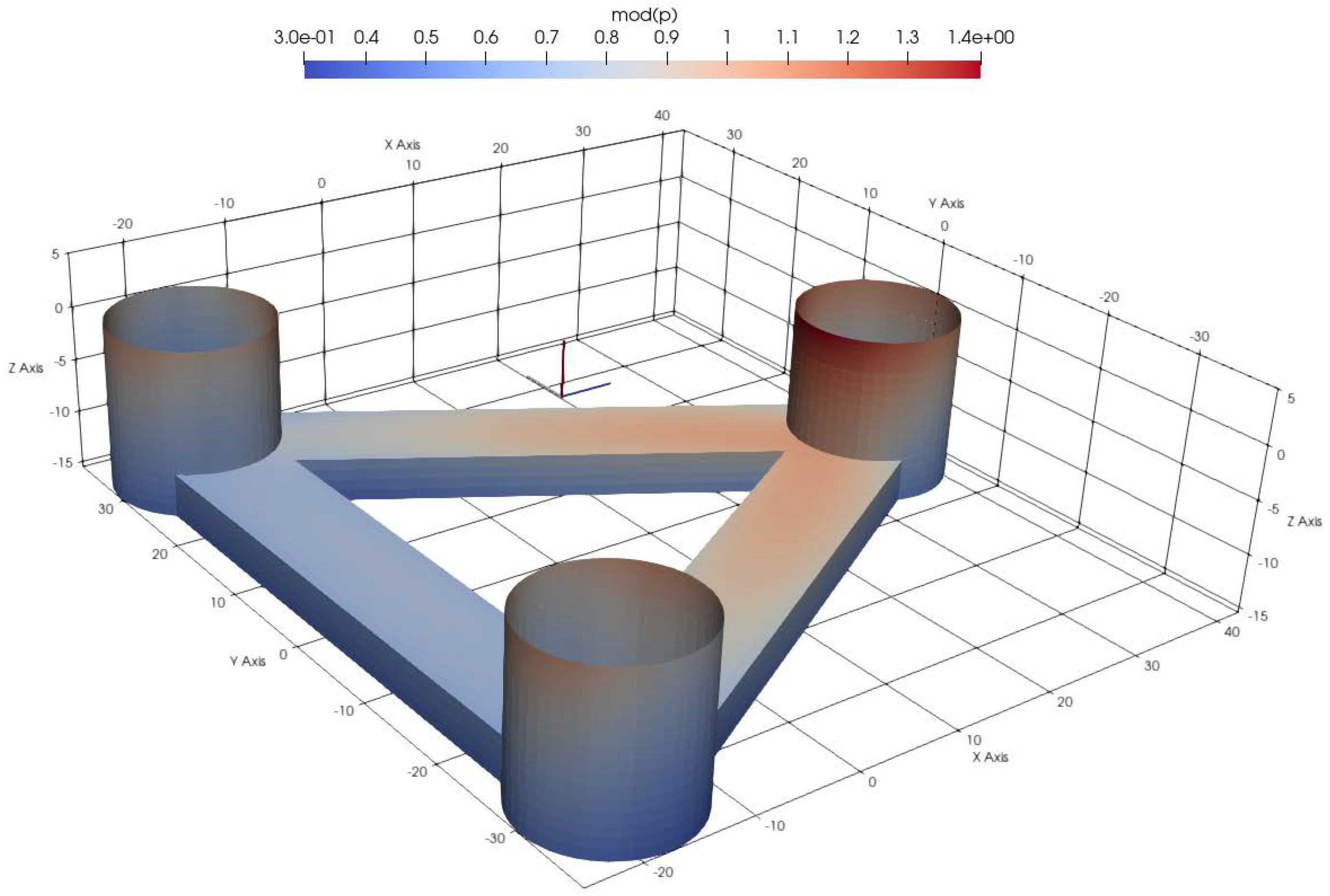
2. Problem Definition

The problem of forces on a floating offshore wind turbine structure fixed in waves is considered in the present study, with the aim to identify the contribution of nonlinear kinematics and viscous forces. To this end, both viscous (CFD) and potential flow solvers are used to calculate forces on the columns, and the results are processed to extract the Morison’s model coefficients.

The structure studied in WINDMOOR research project is selected for this purpose. The structure has a triangular shape composed of three vertical columns joined at the bottom by pontoons and at the top by deck beams (Figure 1). The dimensions of the structure are listed in

Table 2. Main dimensions of the structure presented in full scale.

Platform Height	($PH$)	31 m
Column Diameter	(D)	15 m
Column-Column Distance	($CW$)	61 m
Draft		15.5 m
Pontoon Width		10 m
Pontoon Height		4 m
Deck beams Width		3.5 m

. The structure’s draft is set to 15.5 m in a water depth of 150 m.

The waves are assumed to be traveling in the positive x-axis. Therefore, two of the three columns are placed upstream, symmetric to the $xz$-plane, while the third column is downstream with its center on x-axis (see Figure 2). Here, the two first columns are referred to as Starboard and Port, for negative and positive y coordinates, respectively. The third column on x-axis is referred to as Tower.

The waves are modeled and initialized in the computational domain using the fifth-order Stokes theorem. The particulars of the considered waves in terms of height (H), period (T), and inverse of the steepness ratio ($S=H/\lambda$) are given in

Table 3. Selected wave condition. $KC=VT/D$, $Rn=DV/\nu$, $\beta =Rn/KC$.

Wave	H [m]	T [s]	$\mathit{\lambda }/\mathit{H}$	$\mathit{\lambda }/\mathit{D}$	$\mathbf{KC}$	$\mathit{\beta }$
ID					Nominal	$\times {\mathbf{10}}^{\mathbf{7}}$
W1	1.85	13.33	150	18.50	0.38	1.69
W2	5.55	13.33	50	18.50	1.13	1.69
W3	13.88	13.33	20	18.50	2.77	1.69
W4	1.04	10	150	10.41	0.21	2.25
W5	3.12	10	50	10.41	0.62	2.25
W6	7.81	10	20	10.41	1.55	2.25
W7	17.35	10	9	10.41	3.17	2.25

, where $\lambda$ is the wave length. In addition, Table 3 lists the nominal Keulegan–Carpenter number for each wave, i.e., $KC=VT/D$, where D is the column diameter, T is the wave period, and V is the amplitude of the linear wave particle velocity at the free surface ($z=0$). For the considered waves, the range of the nominal $KC$ number varies between $0.21$ for W4 and $3.17$ for W7.

Due to the variation in the wave particle velocity along the column, the $KC$ number experienced by the column sections differs from the nominal value. The sectional $KC$ is calculated based on the maximum particle velocity at each section (Z coordinate), predicted by linear wave theory.

The $KC$ number could be understood as the ratio between the distance a fluid particle is traveling and the structure’s diameter, or characteristic length. As discussed by Sarpkaya [21] among others, in an oscillatory flow with a large $KC$ number, boundary layer separation and vortex formation are expected. On the other hand, for very small $KC$ numbers, the boundary layer does not have time to fully form and separate, and the force is dominated by the inertia or diffraction effects. Although the $KC$ numbers are relatively small for wave-induced velocities on columns, the small viscous force contributes significantly to drift forces at low frequencies. Therefore, it is important to account for the viscous effect in calculating drift forces.

Another important parameter dictating the boundary layer regime is the Reynolds number. In the present study, the nominal Reynolds number is defined as $Rn=DV/\nu$, where $\nu$ is the water’s kinematic viscosity. In oscillatory flows, the frequency parameter $\beta$ is usually used instead of $Rn$, which is defined as $Rn/KC$. The last column of Table 3 shows this frequency parameter for the studied waves.

The force acting on a column section due to traveling waves ($F^{2D}$) could be decomposed into potential, viscous drag, and residual forces (Equation (2)):

$$F^{2D}=F^P+F^{Dv}+F^R$$

(2)

The potential part, or $F^P$, represents the portion of the force obtained from the potential flow problem solution, namely, diffraction forces in the present problem. The viscous drag force, or $F^{Dv}$, is a representative of the quadratic drag term present in the Morison equation to capture the forces due to viscosity and flow separation (Equation (3)). The inertia part of the Morison model is already considered in the potential part of the force:

$$F^{Dv}={\displaystyle \frac{1}{2}}\rho D{C}_D{u}_r\left|u_r\right|$$

(3)

The residual forces, or $F^R$, represent the remaining part of the force. This includes both potential and viscous higher-order terms. Examples of potential higher-order terms are nonlinear wave kinematics and run-up, while those higher than quadratic viscous forces are examples of the remaining viscous-related force terms. These residual forces are usually neglected in most state-of-the-art simulation tools, mainly because they are difficult to capture accurately with the present simplified models. Here, these components are assumed to be negligible. The viscous flow solution is obtained using CFD in order to calculate $F^{2D}$, whilst the potential flow solution is used to estimate and remove $F^P$ before fitting the remaining force to the quadratic drag force model in order to obtain $C_D$ for each cross section. The adopted methods are described in the following sections.

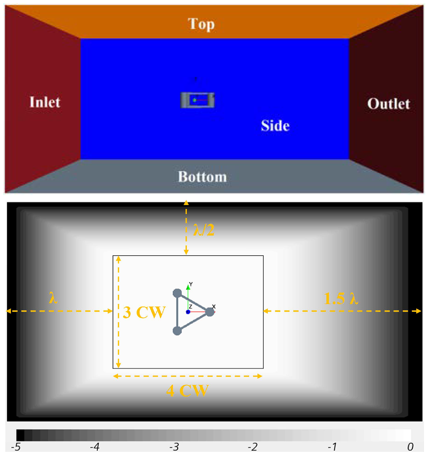
2.1. CFD Numerical Setup

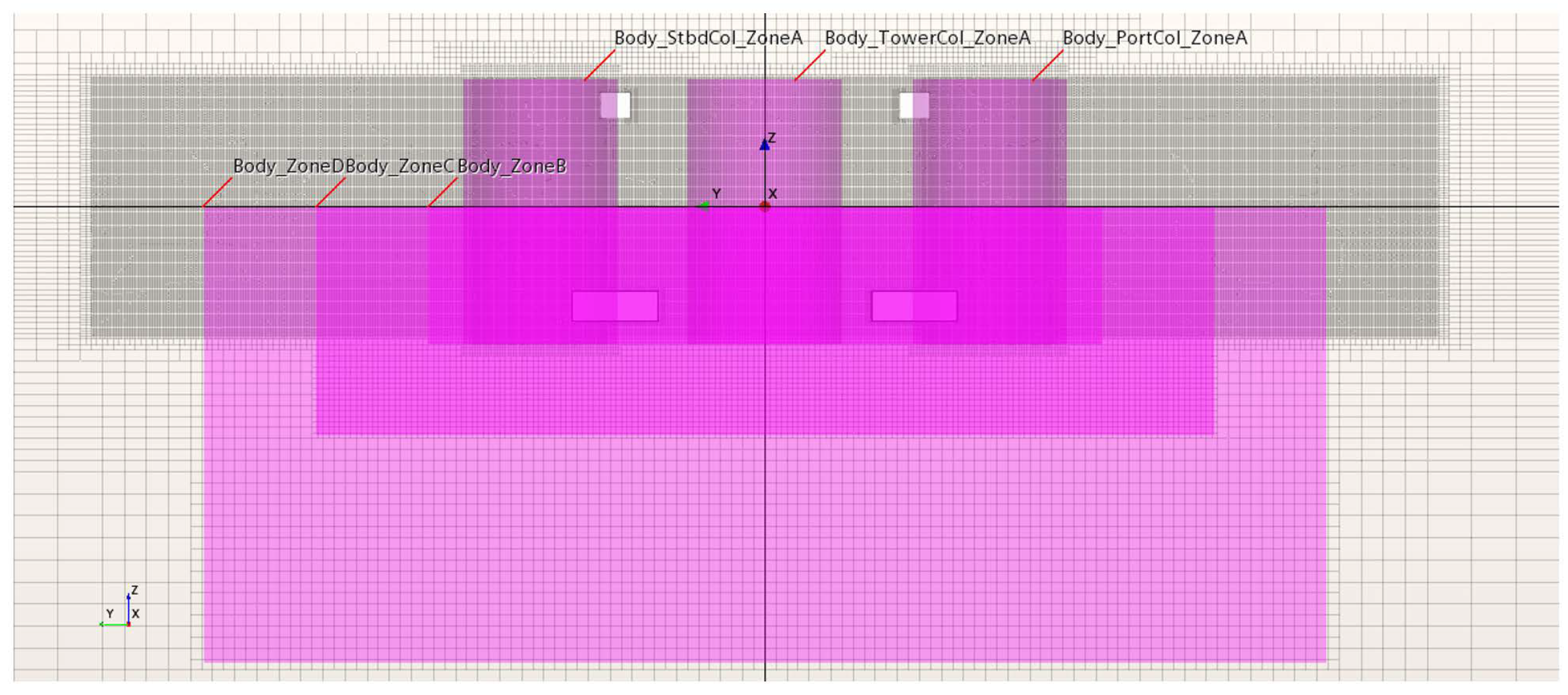
The selected computational domain consists of an inner and an outer domain. The inner domain is centered at the platform center with dimensions of 4 and 3 times the distance between column centers, i.e., 61 m. This inner domain is extended by 1, 1.5, and 0.5 wave lengths of the longest considered wave at the inlet, outlet, and side boundaries, respectively (see Figure 2). The condition on the lateral boundaries of the outer domain (inlet, outlet, and sides) is satisfied by enforcing the velocity field and elevation of the selected regular waves calculated using the fifth-order Stokes solution. In this way, incoming waves are imposed, and outgoing waves are extracted from the domain. However, since the calculated waves are different from the theoretical solution due to diffraction and numerical inaccuracies, the waves must be treated before reaching the boundaries of the outer domain.

The Euler Overlay Method is adopted to gradually blend the prescribed values at the outer domain with the computed numerical solution until the boundaries of the inner domain. A forcing function $F\left(x\right)=\mu cos{(\pi /2x)}^2$ is introduced in the blending zone, where x is the normalized distance from the outer domain boundary and $\mu$ is a constant (see Figure 2). For $x=0$ (at the outer boundary), the solution is equal to the one assigned at the boundary, whereas in the inner domain ($x=1$), the solution is solely computed by CFD. In between the boundaries of the outer and inner domains (blending zone), the forcing function $F\left(x\right)$ is applied to blend the theoretical and numerical solutions. In this way, the diffracted waves are gradually removed from the solution in the blending zone before reaching the boundaries. More details of the method can be found in [22].

All CFD simulations are carried out on a model scale of 1:40 (Froude scaling), while the full-scale dimensions of the WINDMOOR structure are given in Table 2. Unless otherwise specified, all dimensions and results are given in full scale. This means the actual imposed $\beta =Rn/KC$ values in the simulations differ from the full-scale values reported in Table 3.

A velocity condition is imposed on the boundaries with the inlet and outlet in Figure 2. These boundaries are defined in the yz plane and perpendicular to the wave propagation direction. A constant pressure outlet condition is imposed on the top boundary, while the side boundaries are modeled as symmetry planes. The surface of the wind turbine platform is represented with a no-slip wall condition, while a free-slip condition is used on the bottom.

Simulations are run with the software Simcenter STAR-CCM+ 2020.3 Build 15.06.007. The volume of fluid (VOF) method is used to capture the interface between air and water, using a high-resolution interface capturing (HRIC) convection scheme. The turbulent flow is solved using an improved delayed detached eddy simulation (IDDES), resolving the large scales of turbulence whilst modeling small-scale motions. A low-Reynolds number approach is used for the near-wall treatment, requiring a fine near-wall mesh height. An implicit unsteady solver with second-order temporal discretization is used to solve the transient problem, with a constant time-step of $T/500$, where T is the wave period.

2.2. CFD Mesh

A block-refinement methodology is adopted to generate the boundary fitted mesh. The structure’s geometry, boundary layer, and presence of waves, impose different criteria for the generated cell sizes. The refinement strategy provides the possibility to control the cell size in different regions and meet these requirements. The cells’ base size used to discretize the numerical domain is selected based on the columns diameter and summarized in

Table 4. Mesh surface discretization and cell sizes.

	Base Size Ratio	Full Scale	Model Scale
	%	[m]	[m]
Base	100%	3	0.075
Free Surface	2.7%	0.08	0.002
Columns	2.7%	0.08	0.002
Pontoons	5.3%	0.16	0.004
Deck beams	10.7%	0.32	0.008

. The base size is chosen as 20% of the column’s diameter. The sizes of cells on different surfaces after refinement are listed as absolute values in full and model scales, as well as the ratio of the base size.

Numerical simulations and selected mesh refinements are carried out following best practices in SINTEF Ocean for the application of CFD to these problems (see, for example, [23]). For the waves at least 120 cells per wave length and 20 cells per wave height, a target $x/z$ ratio of 2 is ensured. Moreover, at least 500 time steps are performed within one wave period. In order to capture the boundary layer on the structure walls, a prismatic layer is generated around the columns and the pontoons. The near-wall layer has a height of 1.0 $\times {10}^{-4}$ m with the aim to achieve a $y+$ value of 1, where a DES turbulent model with a near-wall treatment could be used. A total of 10 layers are built with a stretching ratio of 1.2 (see the view of the mesh in Figure 3). The mesh size on the body surface and in the domain is chosen after a convergence study carried out on the fixed structure with a constant current, based on SINTEF Ocean best practices. The choices are further controlled for a freely floating platform by running 6DOF simulations with two different grid sizes, the present one and another grid with doubling the refinement. Validation of the results towards model tests are carried out on the decay tests and presented in [24].

2.3. Force Calculation

Pressure on the columns is integrated at each time step to obtain the forces. Each column is split into 23 sections with an equal height of 1 m along its length, where sectional forces are calculated. These sections are numbered as $z_j$, where j is the vertical distance of the center position from the water line such that $z_0$ corresponds to a section with its center on the mean free surface (see Figure 4). In addition to the sectional forces, the total forces on columns and pontoons are extracted.

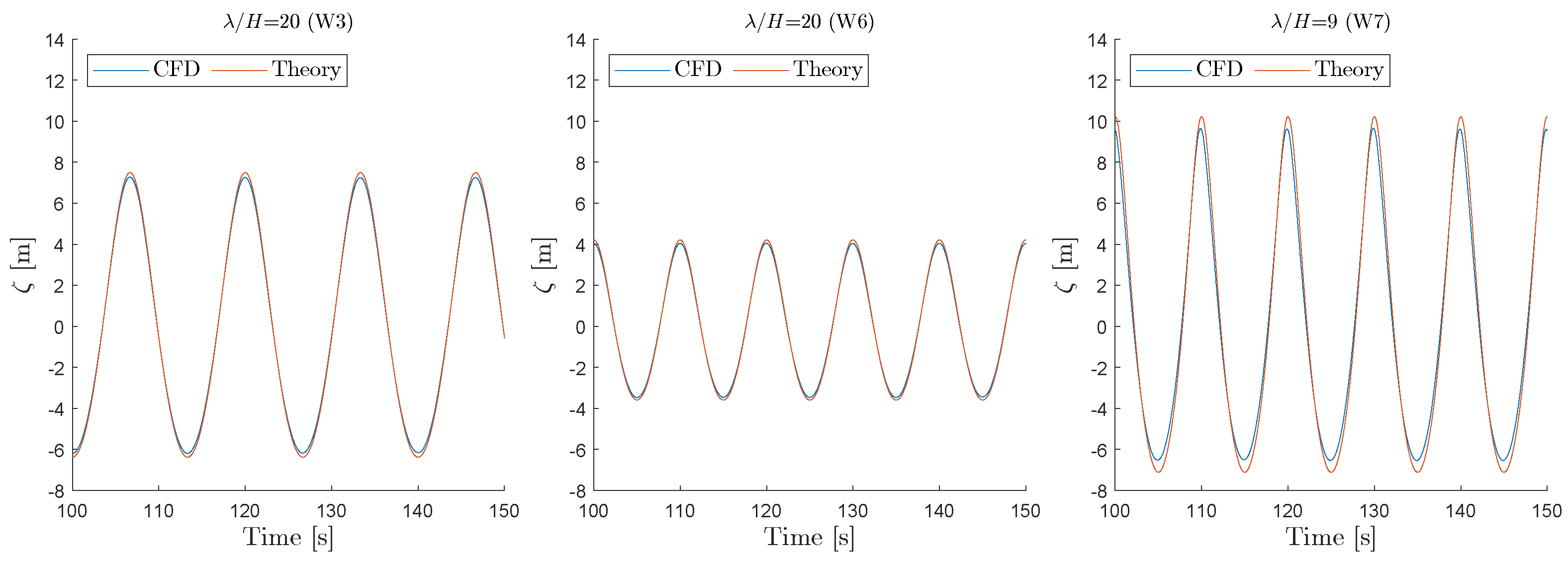
2.4. Wave Kinematics

The kinematics of incident waves on each section are needed for decomposing the obtained forces into mass and drag coefficients, i.e., fitting Morison force model. Therefore, propagation of the target waves are solved without the presence of the structure by imposing the relevant boundary conditions. These are refereed to as “wave-only” simulations. In this way, the simulated kinematics of the waves are recorded to reflect the magnitude of surface elevation at the center of columns, and the center of FOWT as captured by CFD. In addition, the wave-induced particle velocities at the center of the segments along the three columns are recorded. These values are later used as the ambient wave-induced particle velocities when extracting the coefficient from obtained forces where the FOWT is present in the simulations. The surface elevation at the columns is used to determine the wet length and segments on each column.

2.5. Potential Flow Solution

To better understand the contribution of viscous and other nonlinear forces, a linear potential flow solution of the problem is obtained using the boundary element method (panel method). The FOWT surface is discretized in flat panels. The diffraction problem, i.e., fixed FOWT exposed to waves, is solved using WAMIT (v7.3) (ref. [25]). The transfer function of forces on the columns as well as the pressure distribution on the panels of the columns are extracted. The pressure transfer function is later processed, together with the selected wave conditions, and integrated to obtain the time series of potential flow forces on different sections along the columns. These time series of forces are used to subtract the linear potential flow effects from the CFD sectional force time series. The remaining force is then decomposed using the Morison force model into a quadratic drag coefficient and a residual force.

3. Results and Discussions

Forces along the columns for the studied cases are extracted and discussed in this section. The forces are decomposed into potential and quadratic drag forces, and drag coefficient is extracted, using the methodology described in Section 2.

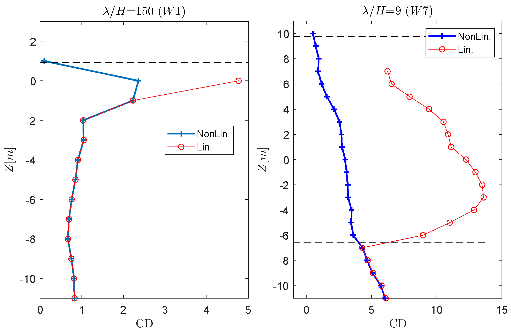
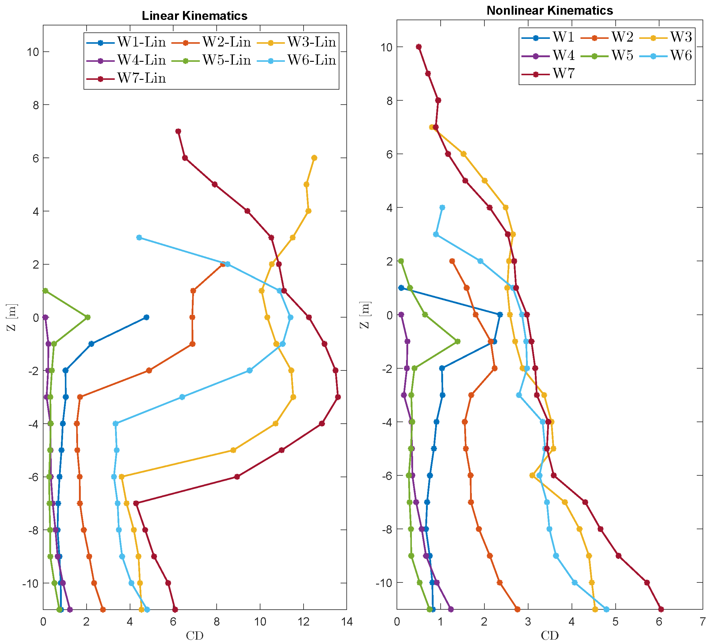
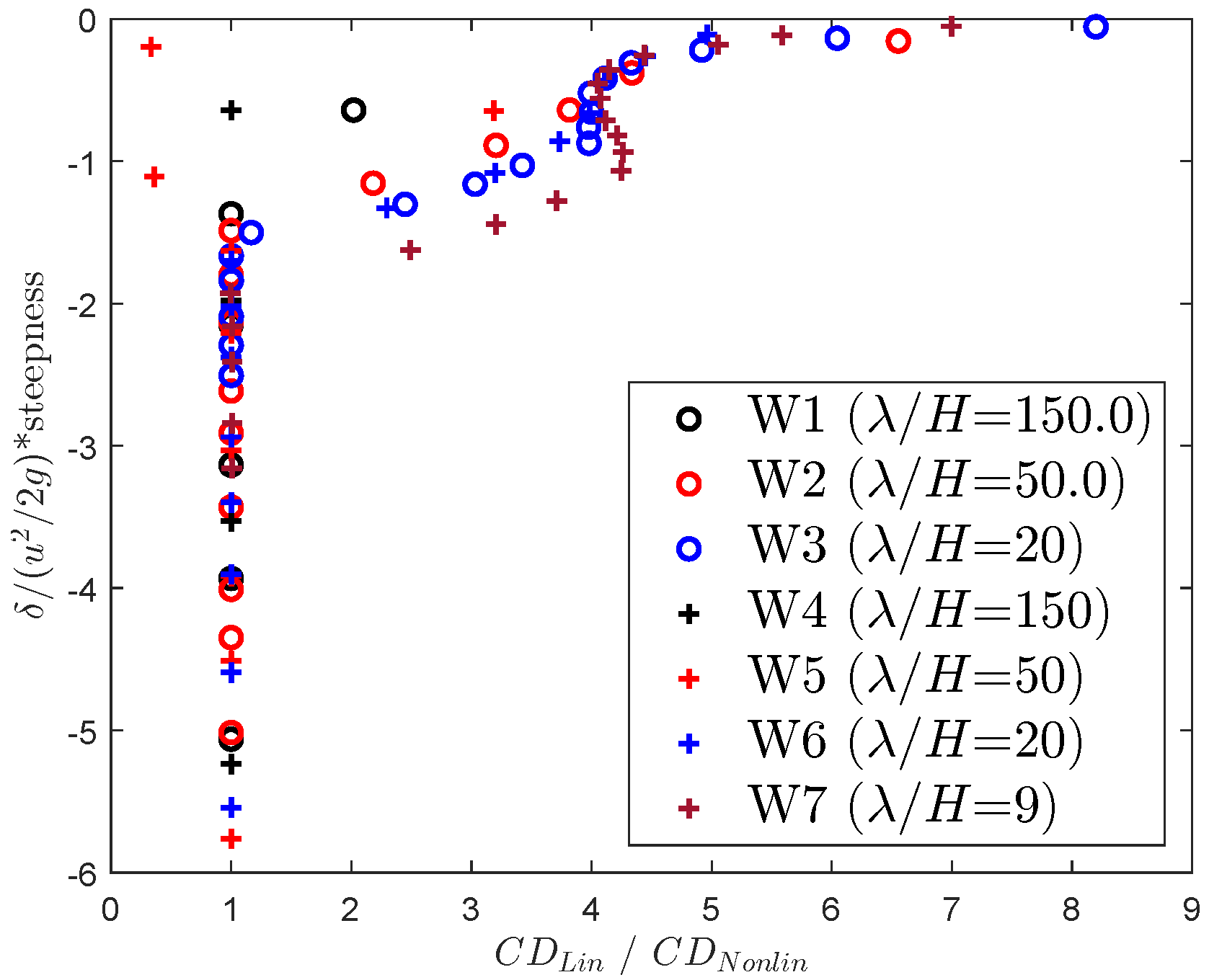
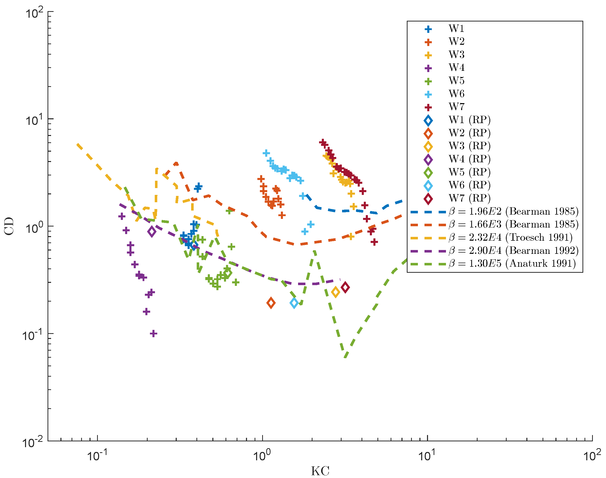
3.1. Drag Coefficients Along the Columns

Figure 5 shows a sample of the obtained force time series for different segments along the starboard column. The corresponding undisturbed free surface elevation at the platform location is shown in Figure 6. The results from the CFD calculations in the absence of a platform are included together with theoretical waves based on the fifth-order Stokes solution. As expected, the nature of the force changes drastically depending on the section’s vertical location and the wave steepness. For higher waves with higher steepness, larger portions of the column go in and out of water. The force drops to zero when the column is dry. For lower sections, in long waves, the force resembles a Morison’s force model signal, oscillatory with slight asymmetry due to the quadratic drag term.

The forces shown in Figure 5 are the total two-dimensional force on a column segment and can be decomposed as proposed in Equation (2). The potential flow diffraction problem is solved using WAMIT (v7.3), and the pressure distribution of the column is extracted. A sample of the obtained pressure distribution over the columns for a 10 s wave is presented in Figure 7. The wet segments are identified by comparing the vertical location of each segment’s center to the undisturbed incident wave elevation at the column location obtained from wave-only CFD simulations. This means that the partially wet segments, as well as water run-up effects, are not properly captured.

The obtained pressure is integrated over the wet horizontal segments. Since the linear solution only provides pressure distribution up to the mean free surface, the pressure values for higher segments are assumed to be constant and equal to the ones on the mean free surface. Considering the amplitude and phase of the incident wave in the origin of the coordinate system, the complex values of pressure are turned into time series for each segment. Special attention is devoted to ensuring that the wave in CFD and potential flow solution are in phase. Figure 8 shows a comparison between the obtained potential flow force on each segment, in addition to the CFD calculated forces. The modified potential flow force is also included. These signals are identical to potential flow forces, as long as the segment stays wet, and set to zero when the segment is above undisturbed wave elevation.

The quadratic drag and residual force on each segment are obtained by subtracting the potential flow force from the total force obtained from CFD, assuming the residual force is negligible (see Equation (2)). Then, Equation (3) is used to calculate a drag coefficient for each segment. The choice of wave kinematics, i.e., $u_r$ in Equation (3), is essential in extracting the drag coefficients.

Let us start by focusing on W1, a relatively linear wave with the nominal KC of 0.38. Figure 9 shows the obtained drag coefficients along the starboard column using the nonlinear wave kinematics obtained from the wave-only CFD simulations. Meaning, the velocities used for $u_r$ are the nonlinear solution of the fluid particle velocities due to propagating undisturbed waves at the location of the column. In addition, the same results using liner wave kinematics are included, marked with “Lin.” in this figure. As expected, for this relatively linear wave with a steepness ratio of 1/150, the obtained drag coefficients are relatively constant away from the splash zone. This area is marked in the figure with dashed lines at the nominal amplitude of the incident wave. Moreover, the predicted values from the linear and nonlinear kinematics are almost identical, except in the splash zone where fluid velocities are under-predicted by linear wave theory, and consequently, larger drag coefficients are obtained.

Unlike the linear version, the drag coefficients obtained using nonlinear wave kinematics are decreasing after entering the splash zone. This is more clearly shown for W7 in Figure 9. The difference between adopting linear or nonlinear wave kinematics is much more evident in this case where the wave steepness equals 1/9.

Figure 10 shows the obtained drag coefficients for different segments along the starboard column for all considered waves, which shows how the general trends observed for W1 and W7 are present in other conditions.

The variation of force coefficients along a column in waves have been also reported before by Dadmarzi et al. [26]. However, here, the contribution from potential flow effects is removed. The remaining drag force still varies along the column, whilst the variations are smaller for the waves with lower steepness.

A non-dimensional distance to the free surface (${\sigma }^{\prime }=\sigma /(u^2/2g)$), as introduced in [27], is used to evaluate the effect of wave kinematics in extracting drag coefficients. Figure 11 shows the ratio between the drag coefficients extracted using linear and nonlinear wave kinematics. Here, $u^2/2g$ represents the fluid velocity head at the free surface, while $\sigma$ is the distance from the undisturbed incident free surface. The ratio of the two drag coefficients is equal to one when the ${\sigma }^{\prime }$ is lower than $-1$. Close to and above ${\sigma }^{\prime }=-1$, which roughly represents the splash zone, the ratio starts to increase and follow a “S-shaped” trend with an inflection point at $CD\left(Lin\right)/CD\left(Nonlin\right)=4$. In engineering applications using linear wave kinetics, often the drag coefficient in the splash zone must be increased to properly represent the forces (see, for example, [28]). Figure 11 suggests that when using linear wave kinematics for calculating forces in the splash zone, the drag coefficient must approximately be increased four times to take the effect of nonlinear kinematics into account. A similar factor is also reported and used by Wang et al. [2].

Figure 12 shows a comparison of the reported drag coefficients for an oscillatory cylinder in infinite fluid in the literature. The reported values are for pure single frequency, harmonic, two-dimensional flow, where $\beta$ values are from approximately $2\times {10}^2$ to $1.3\times {10}^5$. The full-scale $\beta$ values are outside this range (about $2\times {10}^7$), while the model-scale values are within (about $2\times {10}^4$). Disregarding the discrepancies in the reported values for $\beta >={10}^4$, it seems the drag coefficients are less dependent on $\beta$. The recommended values from [5], marked with (RP) are also included for the nominal $KC$ numbers of the waves, which seem to follow the reported values for $\beta >={10}^4$.

The extracted drag coefficients for the segments along the starboard column for all the considered waves are shown with a plus sign in Figure 12. Since the incident wave particle velocity changes along the column, a range of $KC$ numbers is obtained for each wave. For a column with a constant cross section as shown here, the higher $KC$ numbers indicate that the segment is closer to the free surface, i.e., experiences higher fluid velocity. For the lowest steepness of 1/150, i.e., W1 and W4, the drag coefficients for lowest $KC$ values are in good agreement with the Recommended Practice [5] and experimentally reported values. However, as the $KC$ increases, i.e., the segment gets closer to the free surface, the magnitude is deviating from the expectation. It seems that the variation depends both on steepness as well as the wave-length-to-diameter ratio. The drag coefficients for waves with higher steepness start with a much higher value than expected and are generally decreasing for higher $KC$ numbers. This could be attributed to the free surface effects, and the fact that pressure on the free surface has to stay constant. It is possible to conclude that other phenomena besides quadratic drag are present in the interaction between fluid and the segments, especially in the presence of the free surface. The fact that a quadratic model has chosen to represent the resulted force leads to obtaining higher than previously estimated drag coefficients, which decreases as the segment gets closer to the free surface. This suggests the variation in drag coefficients along the column cannot be explained by $KC$ alone.

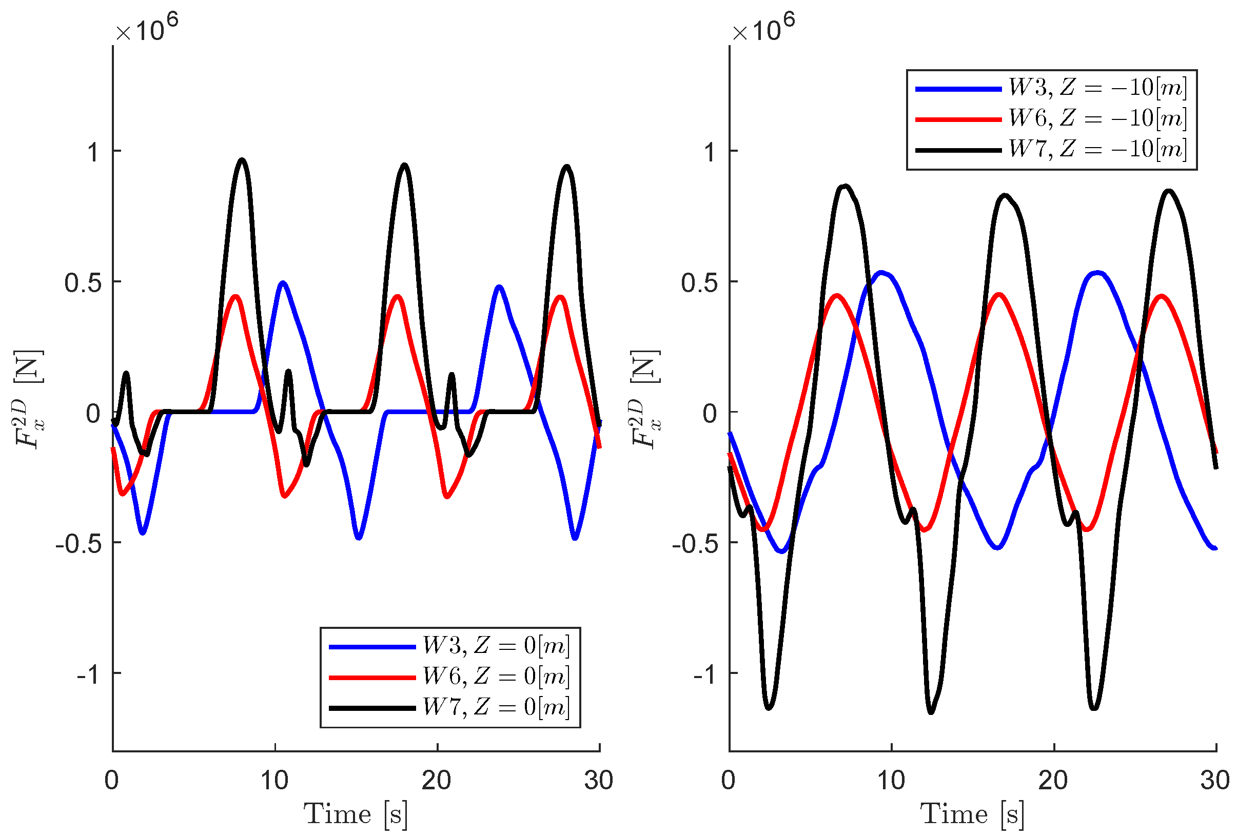
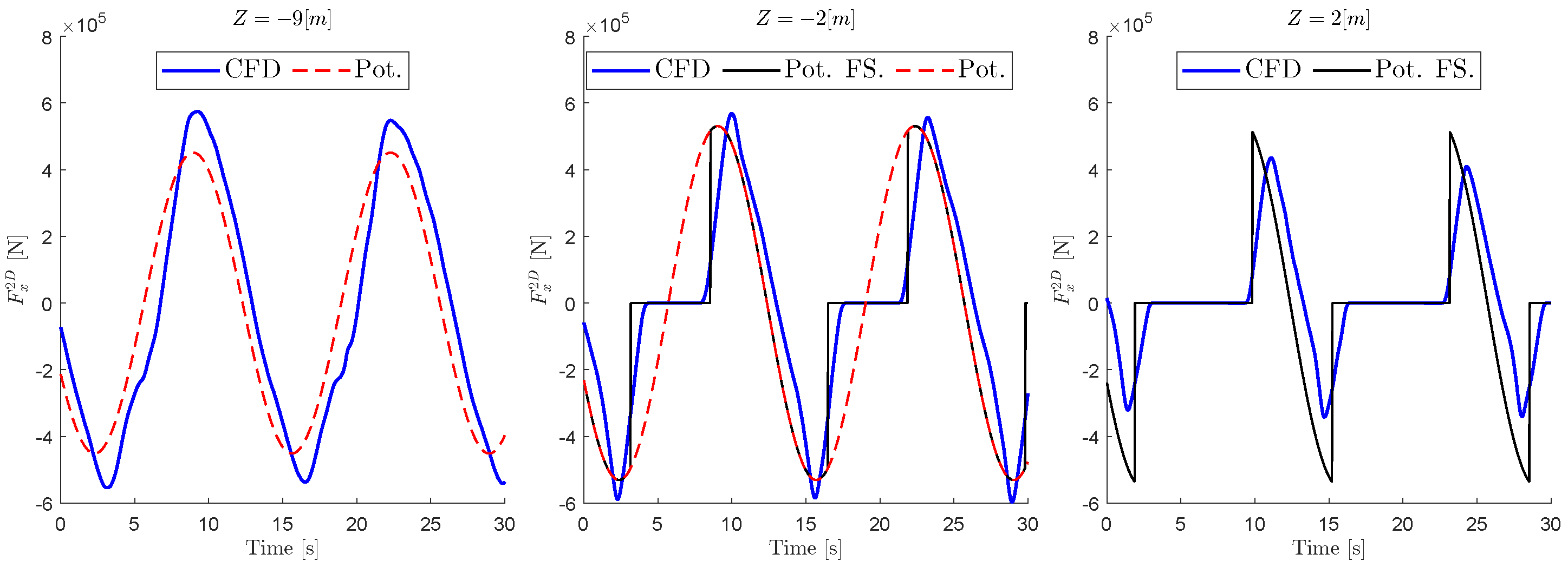
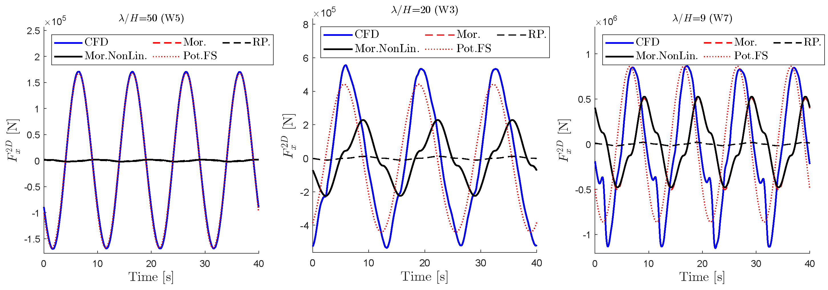
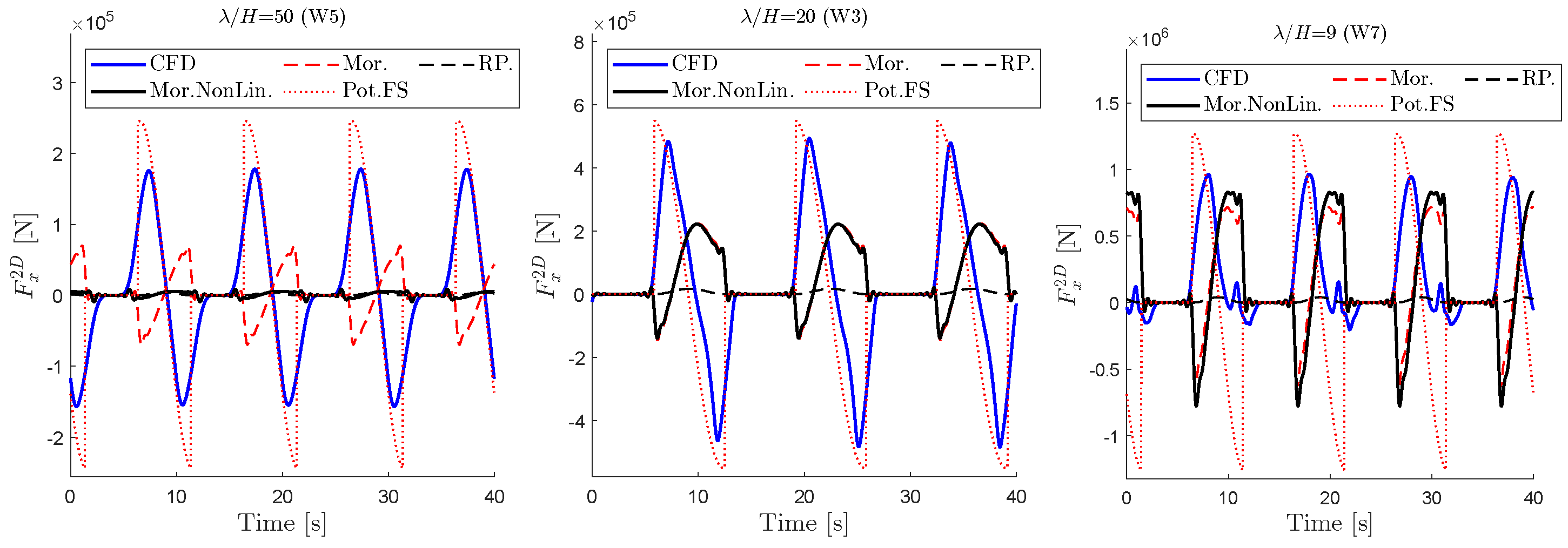
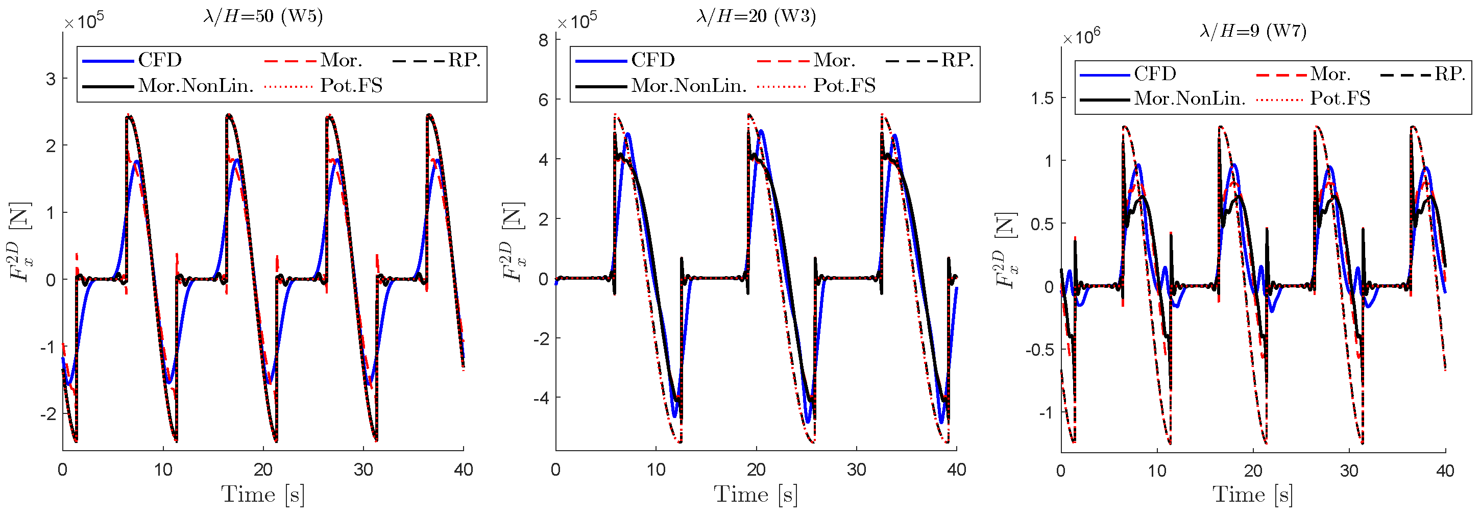
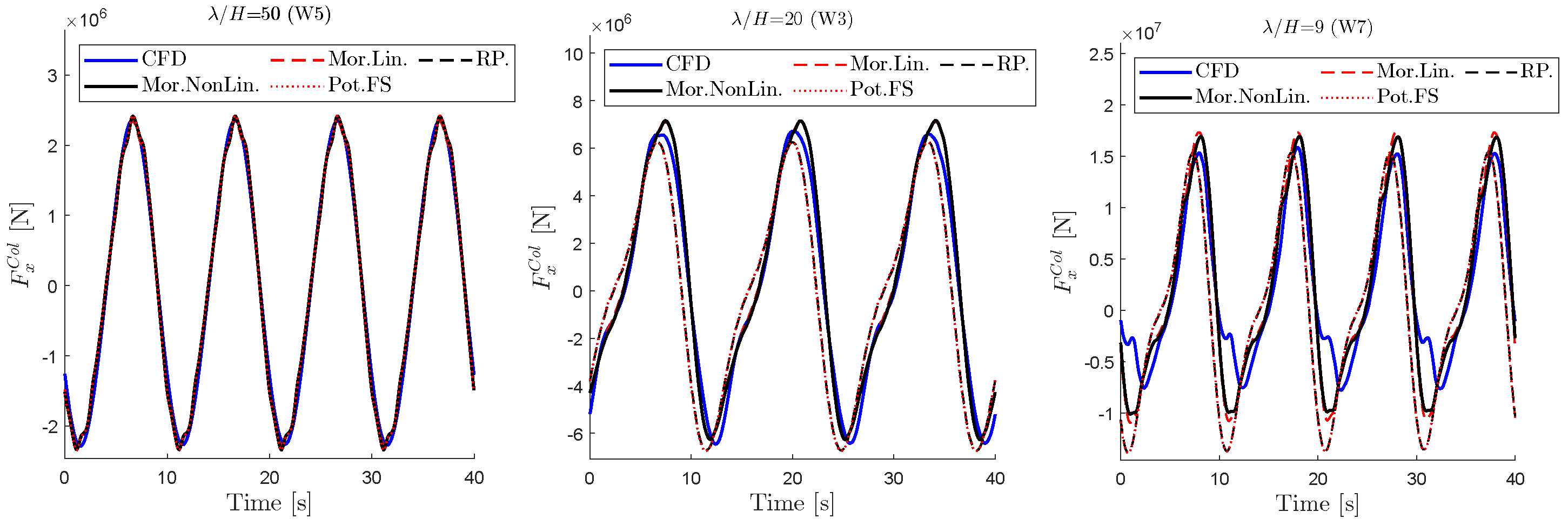
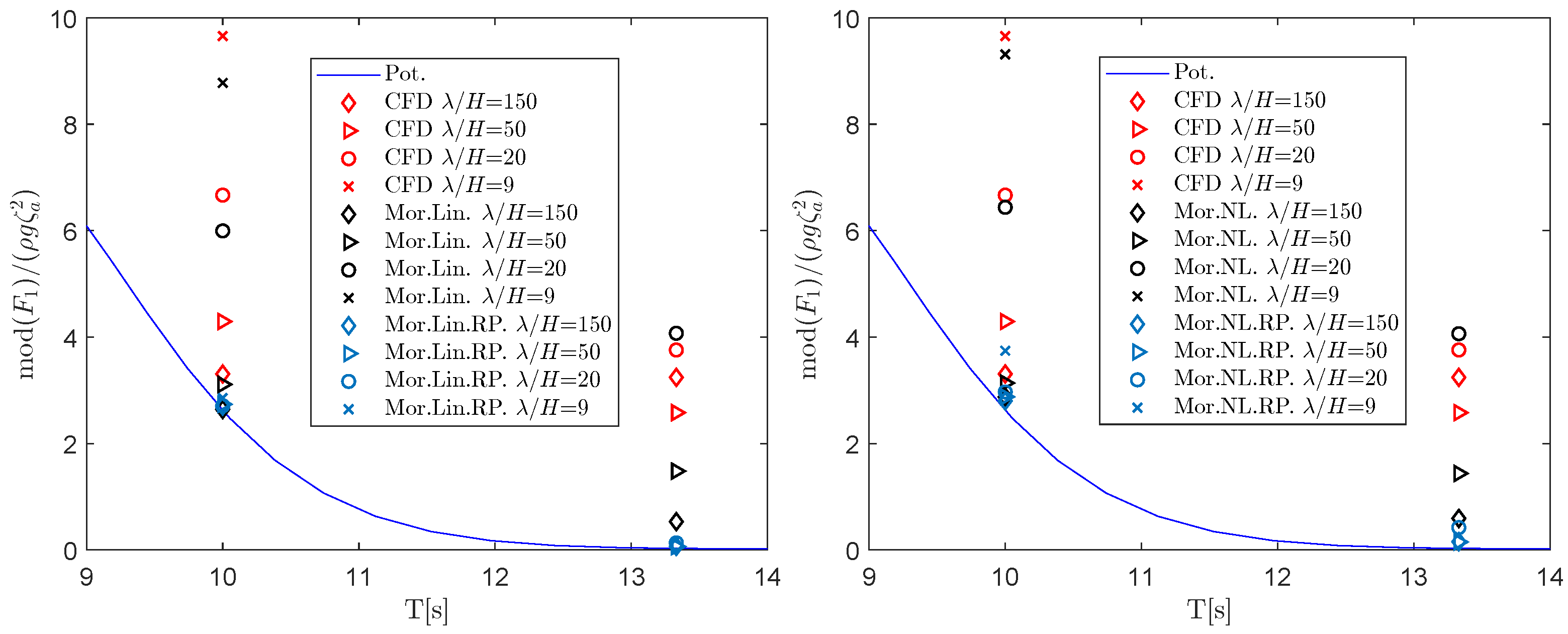
3.2. Reconstructed Forces

Figure 13 shows the x-component of the force time series on the lowest segment of the starboard column (Z = $-10$ m) for three different waves. The forces obtained from CFD as well as the diffraction forces from potential flow and the extracted quadratic drag term are included for comparison. Three different method for calculating the drag force are presented, while all three are using the Morison drag model. The included force components are as follows:

• Linear Diffraction (Pot.FS.): Linear diffraction forces calculated using potential flow theory and stretched up to instantaneous free surface.
• Linear Morison (Mor.): The drag coefficient is extracted using linear wave kinematics, and forces are calculated with linear wave kinematics.
• Nonlinear Morison (Mor. NonLin.): The drag coefficient is extracted using nonlinear wave kinematics, and nonlinear wave kinematics are used for calculating forces.
• Linear Morison with Recommended Practice drag coefficient [5] (RP): Linear wave kinematics and the recommended drag coefficient are used to calculate forces.

Starting with the wave with the lowest steepness, i.e., W5, the segment is sufficiently far away from the splash zone for the influence of drag to be negligible, and therefore the potential force agrees well with the CFD results. As expected, the importance of the drag term increases with the steepness, i.e., W3 and W7. The linear and nonlinear Morison drag forces give very close results, while the predicted drag force using the recommended coefficients from [5] is much smaller. The phase difference between the drag and potential force is noticeable. The phase of the CFD force is slightly behind that of the potential force while it is ahead of the drag term.

Figure 14 shows the reconstructed force by adding the potential flow force to the calculated drag components. As expected, the force for the lowest segment matches well with the CFD results due to the small contribution of the drag force. In cases with higher-steepness waves, the phase of the total force is much closer to the CFD results by adding the potential force. The linear and nonlinear Morison models give similar results and match the CFD forces in terms of phase and amplitude reasonably well. However, for W7 with the highest steepness, it is clear that there are complex phenomena which cannot be captured, particularly when the flow is moving back, i.e., when the wave is passing. The CFD results seem to suggest the presence of a secondary wave system, interacting with the segment. Such a phenomenon has been reported before in [29] for steep waves interacting with columns.

Figure 15 shows a similar comparison for a segment on the mean free surface, i.e., Z = 0 m. Here, the linear diffraction forces (Pot.FS.) and the drag component seem to cancel each other. The difference between the linear and nonlinear Morison models for the lowest steepness is noticeable. This difference is much smaller for the cases with higher steepness. It is possible to argue that the nonlinear Morison model gives better, and more physically correct, drag forces. However, comparing the reconstructed forces in Figure 16 suggests that a consistent order of modeling for drag and diffraction forces matters. This means that combining the linear diffraction forces and linear Morison (please see the definition above) gives better local predictions, at least when potential flow diffraction forces are dominant.

Figure 17 shows a comparison of the total force on the Starboard column in the x direction, both from the CFD and reconstructed force using different methods. Similar to segment forces, the total force on the column is predicted with good accuracy for the lowest wave steepness. For higher steepness waves, the linear and nonlinear Morison models seem to perform equally well, and better than the other method. However, for the highest steepness (W7), the peak of the negative force is not captured by any of the models.

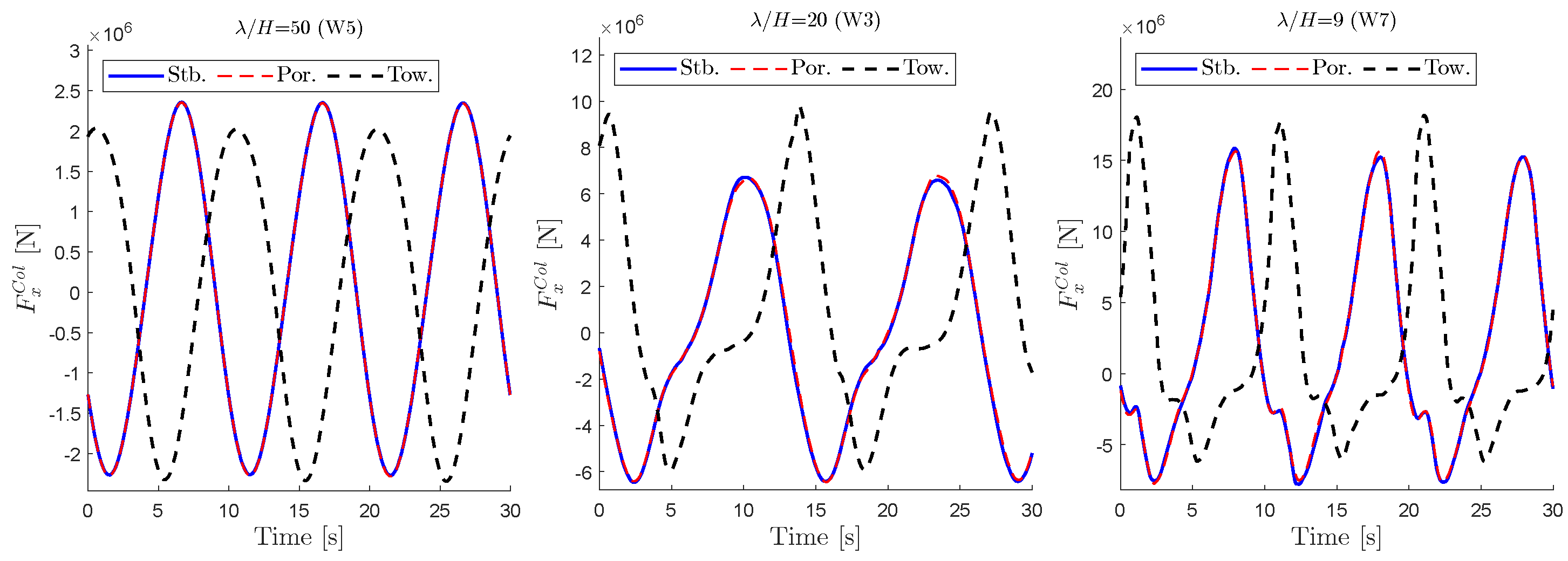
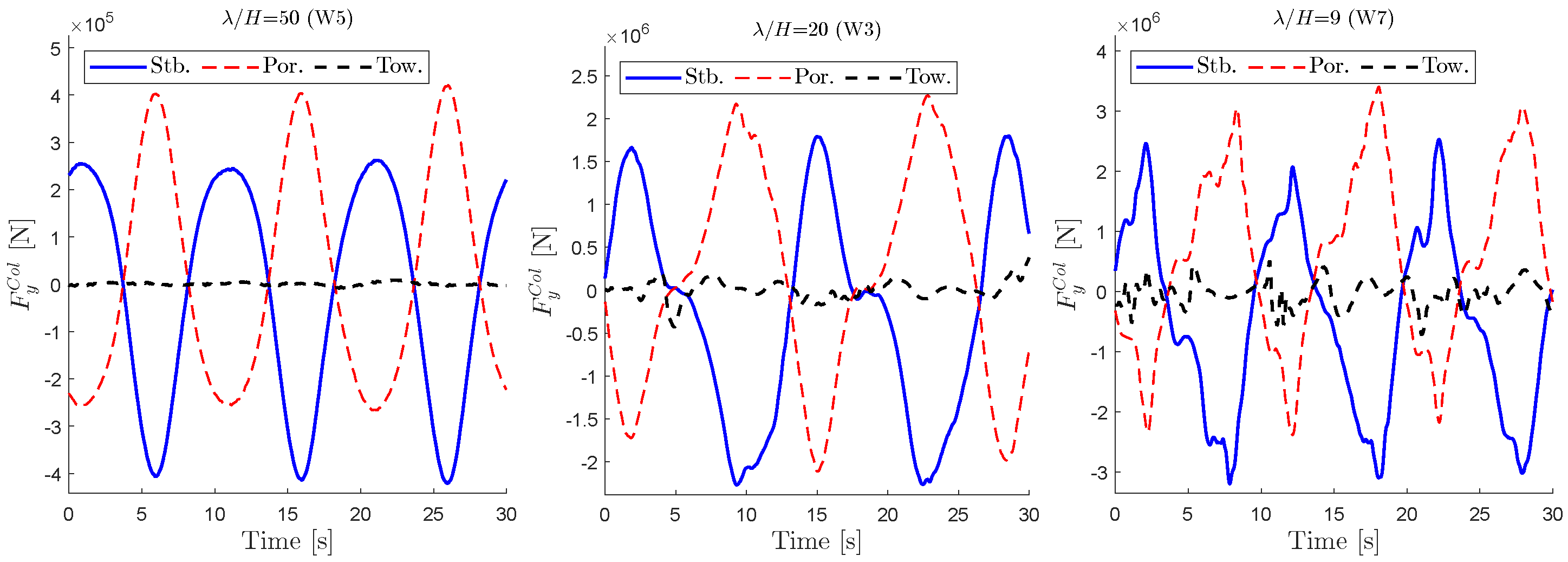
3.3. Interaction Effects

In practice, it is assumed that the effects of the columns diffracted wave pattern on the viscous forces of other columns are negligible. Using CFD, it is possible to evaluate this assumption. Figure 18 shows the obtained total forces in the x direction on the three columns from CFD. The forces on the starboard and port columns are almost identical, while the force on the tower shows a phase shift. In addition to the shift, the magnitude and the shape of the peaks are also different. This could be attributed to the diffraction effects of the upstream columns since using a pure Morison model with the kinematics of the undisturbed wave fails to reproduce such differences.

Figure 19 shows the reconstructed forces from the nonlinear Morison model, together with the linear diffraction solution from potential-flow theory. In this way, the diffraction wave patterns of the columns are included in calculating the forces. The obtained forces show similar differences between the tower and the other two columns, which suggests that including diffraction waves in calculating forces on closely placed columns might be important. This is more clear for the forces perpendicular to the wave propagation direction (y direction for the present cases). Figure 20 shows the obtained forces on the columns in y direction. Although the forces predicted by Morison model after imposing a long crested uniform wave in x direction predict no force in the y direction, the CFD calculation suggests a strong force in y, which is consistent with the potential flow diffraction results. This suggests, depending on the column dimensions, that the diffraction effects, and their consequent effect on viscous forces, cannot be neglected.

3.4. Drift Forces

Viscous forces contribute to mean and low-frequency drift forces. An estimation of the obtained drift force on the columns is presented here. The potential mean drift force on the three columns is calculated using linear potential flow solver WAMIT. In addition, the mean forces from CFD and the constructed forces from the three different method presented in Section 3.2 are shown in Figure 21. Here, the recommended drag coefficients from [5] are used both with linear and nonlinear kinematics. The predicted obtained values from CFD show higher mean drift forces, comparing to the potential flow effects, which could be attributed to the contribution of viscous forces (see, for example, [30]). The linear and nonlinear Morison models, with extracted drag coefficients, give a better prediction of the mean drift forces. However, the values are slightly under-predicted comparing to CFD, while the nonlinear Morison models perform slightly better. In the case of the lowest-steepness waves with the higher period (13.3 s), the under-prediction is larger. Meaning, the mean drift forces by CFD are up to four times larger than the estimation by the Morison models. The exact reason for this difference is not fully understood and left for future investigations. A similar comparison for a higher-steepness wave with the same period gives much closer results. Overall, the results suggest a higher drag coefficient than what is usually applied is needed to reproduce the mean drift forces.

4. Conclusions

The total and sectional forces on columns of a floating offshore wind turbine (FOWT) support structure were investigated using CFD and potential flow. Morison-type models were used to decompose the forces on column sections and extract a quadratic drag coefficient along the column.

It was shown that it is important to consider potential flow forces in processing CFD forces to extract drag coefficients. The exact free surface should be considered while selecting the segments which are wet and hence exposed to wave forces.

Moreover, the residual forces on column could be translated to drag coefficients using linear or nonlinear wave kinematics. The drag coefficient extracted from nonlinear wave kinematics gives a more correct physical representation of the drag force. For example, the forces goes to zero when approaching the instantaneous free surface. The drag coefficients extracted using linear wave kinematics give a more consistent drag force with linear diffraction forces. As a consequence, where linear diffraction forces are important, the reconstructed force using the linear Morison results gives a better prediction of the total force.

It was also discussed that interaction effects due to diffracted waves between different columns may matter, especially for forces perpendicular to wave propagation direction. The potential part of such an interaction could be considered using the potential flow solution of the diffraction problem.

Comparison of the forces with CFD suggested that higher drag coefficients than are recommended in [5] are usually needed, especially close to the free surface, regardless of using linear or nonlinear kinetics. Therefore, it is possible to under-predict viscous contribution to drift forces on large columns if the proper choice of drag coefficients and consistent wave kinematics are not applied. Moreover, it was shown that in steep waves, the quadratic drag model is unable to capture the local forces around the splash zone accurately. For this reason, model testing is an important tool to validate and tune the viscous contribution to drift forces (see, for example, [30]).

As a future study, the drag forces obtained here could be added as a correction to the potential flow drift forces, where the mean drift motion of FOWT can be compared with the measured data of the model test carried out in the WINDMOOR project.

References

1. Ommani, B.; Fonseca, N.; Stansberg, C.T. Simulation of Low Frequency Motions in Severe Seastates Accounting for Wave-Current Interaction Effects. In Proceedings of the International Conference on Ocean, Offshore and Arctic Engineering OMAE2017, Trondheim, Norway, 25–30 June 2017. [Google Scholar] [CrossRef]
2. Wang, L.; Robertson, A.; Jonkman, J.; Yu, Y.H. OC6 phase I: Improvements to the OpenFAST predictions of nonlinear, low-frequency responses of a floating offshore wind turbine platform. Renew. Energy 2022, 187, 282–301. [Google Scholar] [CrossRef]
3. Faltinsen, O.M. Sea Loads on Ships and Offshore Structures; Cambridge Ocean Technology Series; University Press: Cambridge, UK, 1990. [Google Scholar]
4. Ormberg, H. SIMO-Theory Manual Version 4.0 Rev. 1; Technical Report MT51 F93-0184; SINTEF Ocean: Trondheim, Norway, 2012. [Google Scholar]
5. DNV. DNV-RP-C205 Environmental Conditions and Environmental Loads; Technical Report DNV-RP-C205; DET NORSKE VERITAS: Høvik, Norway, 2014. [Google Scholar]
6. Sarpkaya, T. In-Line and Transverse Forces on Cylinders in Oscillatory Flow at High Reynolds Numbers. J. Ship Res. 1977, 21, 200–216. [Google Scholar] [CrossRef]
7. Bearman, P.W.; Downie, M.J.; Graham, J.M.R.; Obasaju, E.D. Forces on cylinders in viscous oscillatory flow at low Keulegan-Carpenter numbers. J. Fluid Mech. 1985, 154, 337–356. [Google Scholar] [CrossRef]
8. Sarpkaya, T. Force on a circular cylinder in viscous oscillatory flow at low Keulegan—Carpenter numbers. J. Fluid Mech. 1986, 165, 61. [Google Scholar] [CrossRef]
9. Chaplin, J.R. Loading on a cylinder in uniform oscillatory flow: Part I—Planar oscillatory flow. Appl. Ocean. Res. 1988, 10, 120–128. [Google Scholar] [CrossRef]
10. Justesen, P. Hydrodynamic Forces on Large Cylinders in High Reynolds Number Oscillatory Flow. In Proceedings of the Behaviour of Offshore Structures ’88, Trondheim, Norway, 3 June 1988. [Google Scholar]
11. Anaturk, A.R. An experimental investigation to measure hydrodynamic forces at small amplitudes and high frequencies. Appl. Ocean. Res. 1991, 13, 200–208. [Google Scholar] [CrossRef]
12. Troesch, A.W.; Kim, S.K. Hydrodynamic forces acting on cylinders oscillating at small amplitudes. J. Fluids Struct. 1991, 5, 113–126. [Google Scholar] [CrossRef]
13. Bearman, P.W.; Mackwood, P.R. Measurements of the Hydrodynamic Damping of Circular Cylinders. In Proceedings of the Behaviour of Offshore Structures ’92, London, UK, 7–10 July 1992; p. 405. [Google Scholar]
14. Chaplin, J.R. Planar Oscillatory Flow Forces at High Reynolds Numbers. J. Offshore Mech. Arct. Eng. 1993, 115, 31–39. [Google Scholar] [CrossRef]
15. Gao, Z.; Efthymiou, M.; Cheng, L.; Zhou, T.; Minguez, M.; Zhao, W. Hydrodynamic damping of a circular cylinder at low KC: Experiments and an associated model. Mar. Struct. 2020, 72, 102777. [Google Scholar] [CrossRef]
16. Nakamura, M.; Hoshino, K.; Koterayama, W. Three-Dimensional Effects on Hydrodynamic Forces Acting on an Oscillating Finite-Length Circular Cylinder. Int. J. Offshore Polar Eng. 1992, 2, 6. [Google Scholar]
17. Vengatesan, V.; Varyani, K.S.; Barltrop, N. An experimental investigation of hydrodynamic coefficients for a vertical truncated rectangular cylinder due to regular and random waves. Ocean. Eng. 2000, 27, 291–313. [Google Scholar] [CrossRef]
18. Paulsen, B.T.; Bredmose, H.; Bingham, H.; Jacobsen, N. Forcing of a bottom-mounted circular cylinder by steep regular water waves at finite depth. J. Fluid Mech. 2014, 755, 1–34. [Google Scholar] [CrossRef]
19. Clément, C.; Bozonnet, P.; Vinay, G.; Pagnier, P.; Nadal, A.B.; Réveillon, J. Evaluation of Morison approach with CFD modelling on a surface-piercing cylinder towards the investigation of FOWT Hydrodynamics. Ocean. Eng. 2022, 251, 111042. [Google Scholar] [CrossRef]
20. Wang, L.; Robertson, A.; Jonkman, J.; Yu, Y.H.; Koop, A.; Borràs Nadal, A.; Li, H.; Bachynski-Polić, E.; Pinguet, R.; Shi, W.; et al. OC6 Phase Ib: Validation of the CFD predictions of difference-frequency wave excitation on a FOWT semisubmersible. Ocean. Eng. 2021, 241, 110026. [Google Scholar] [CrossRef]
21. Sarpkaya, T. Structures of separation on a circular cylinder in periodic flow. J. Fluid Mech. 2006, 567, 281–297. [Google Scholar] [CrossRef]
22. Kim, J.; O’Sullivan, J.; Read, A. Ringing Analysis of a Vertical Cylinder by Euler Overlay Method; American Society of Mechanical Engineers Digital Collection: New York, NY, USA, 2013; pp. 855–866. [Google Scholar] [CrossRef]
23. Bouscasse, B.; Califano, A.; Choi, Y.M.; Haihua, X.; Kim, J.W.; Kim, Y.J.; Lee, S.H.; Lim, H.J.; Park, D.M.; Peric, M.; et al. Qualification Criteria and the Verification of Numerical Waves: Part 2: CFD-Based Numerical Wave Tank; American Society of Mechanical Engineers Digital Collection: New York, NY, USA, 2021. [Google Scholar] [CrossRef]
24. Califano, A.; Berthelsen, P.A.; Magalhaes Duque Da Fonseca, N.M. Effect of body motion on the wave loads computed with CFD on the INO-WINDMOOR floater. J. Phys. Conf. Ser. 2023, 2626, 012034. [Google Scholar] [CrossRef]
25. WAMIT. User Manual; Technical Report Version 7.4; WAMIT, Inc.: Chestnut Hill, MA, USA, 2020. [Google Scholar]
26. Dadmarzi, F.H.; Califano, A.; Fonseca, N.; Berthelsen, P.A. Comparison of Morison Forces with CFD Modelling for a Surface Piercing Column of a FOWT. In Proceedings of the ASME 2022 International Offshore Wind Technical Conference IOWTC2022, Boston, MA, USA, 7–8 December 2022. [Google Scholar]
27. Dean, R.G.; Dalrymple, R.A.; Hudspeth, R.T. Force Coefficients from Wave Project I and II Data Including Free Surface Effects. Soc. Pet. Eng. J. 1981, 21, 779–786. [Google Scholar] [CrossRef]
28. Berthelsen, P.A.; Baarholm, R.; Pa´kozdi, C.; Stansberg, C.T.; Hassan, A.; Downie, M.; Incecik, A. Viscous Drift Forces and Responses on a Semisubmersible Platform in High Waves. In Proceedings of the Volume 1: Offshore Technology, Honolulu, HI, USA, 31 May–5 June 2009; pp. 469–478. [Google Scholar] [CrossRef]
29. Kristiansen, T.; Faltinsen, O.M. Higher harmonic wave loads on a vertical cylinder in finite water depth. J. Fluid Mech. 2017. [Google Scholar] [CrossRef]
30. Fonseca, N.; Stansberg, C.T. Wave Drift Forces and Low Frequency Damping on the Exwave Semi-Submersible. In Proceedings of the Volume 1: Offshore Technology, Trondheim, Norway, 25–30 June 2017; p. V001T01A085. [Google Scholar] [CrossRef]
Figure 1. Platform geometrical model. The wave is propagating in the positive x-direction.
Jmse 13 00264 g001
Figure 2. A view of the computational domain with the rectangle showing the inner domain. C W : column to column distance. λ : longest wave length considered. The magnitude of wave forcing function at the water level is shown with shading. The wave is propagating in the positive x-axis direction.
Jmse 13 00264 g002
Figure 3. Lateral view of the mesh discretization with body volume refinements.
Jmse 13 00264 g003
Figure 4. Horizontal segments along the column.
Jmse 13 00264 g004
Figure 5. Sectional force time series on the starboard column for three waves (W3, W5, W7) and two heights.
Jmse 13 00264 g005
Figure 6. Comparison of CFD and theoretical undisturbed free surface elevation at the middle of the platform. Theory: initialized domain using the fifth-order Stokes wave.
Jmse 13 00264 g006
Figure 7. Amplitude of the pressure over the structure from the potential flow solution of the diffraction problem for a 10 s wave.
Jmse 13 00264 g007
Figure 8. Comparison of CFD and potential forces on several segments along the starboard column for Wave 3. Pot.: Potential force from WAMIT. Pot. FS.: Potential forces stretched up to the instantaneous free surface.
Jmse 13 00264 g008
Figure 9. Drag coefficient for W1 and W7 extracted by decomposing the residual force after removing the potential flow sectional force contribution using both nonlinear and linear (-Lin) wave kinematics. See Table 3 for wave condition details. The two dashed lines show the boundaries of the splash zone.
Jmse 13 00264 g009
Figure 10. Drag coefficient on Starboard column, extracted by fitting a quadratic model to the CFD force after removing the potential flow sectional force contribution using linear and nonlinear wave kinematics.
Jmse 13 00264 g010
Figure 11. Ratio of drag coefficients from linear and nonlinear kinematics.
Jmse 13 00264 g011
Figure 12. Drag coefficient extracted by decomposing the force.
Jmse 13 00264 g012
Figure 13. Comparison of CFD and force components on Z = 10 m segment on the starboard column for Wave 3, 5 and 7.Mor.: quadratic drag using linear wave kinematics. RP.: Same as Mor. but with recommended drag coefficients from [5]. Mor.NonLion.: same as Mor. but with nonlinear wave kinematics. Pot. FS.: Potential forces stretched up to the instantaneous free surface.
Jmse 13 00264 g013
Figure 14. Comparison of CFD and reconstructed forces on Z = 10 m segment on the starboard column for Waves 3, 5, and 7. Legends are the same as Figure 13, and potential forces are added to all drag components.
Jmse 13 00264 g014
Figure 15. Comparison of CFD and force components on Z = 0 m segment on the starboard column for Wave 3, 5 and 7.Mor.: quadratic drag using linear wave kinematics. RP.: Same as Mor. but with the recommended drag coefficients from [5]. Mor.NonLion.: same as Mor. but with the nonlinear wave kinematics. Pot. FS.: potential forces stretched up to the instantaneous free surface.
Jmse 13 00264 g015
Figure 16. Comparison of CFD and reconstructed forces on Z = 10 m segment on the starboard column for Waves 3, 5 and 7. Legends are the same as Figure 15, and potential forces are added to all drag components.
Jmse 13 00264 g016
Figure 17. Comparison of CFD and reconstructed total forces on the starboard column for Wave 3, 5 and 7. Mor.: quadratic drag and potential-flow forces using linear wave kinematics. RP.: same as Mor. but with recommended drag coefficients from [5]. Mor.NonLion.: same as Mor. but with nonlinear wave kinematics. Pot. FS.: linear diffraction forces from potential flow stretched up to the instantaneous free surface.
Jmse 13 00264 g017
Figure 18. Comparison of CFD forces on columns for three waves. Stb.: Starboard, Por.: Port, Tow.: Tower.
Jmse 13 00264 g018
Figure 19. Comparison of CFD and reconstructed forces on starboard (Stb.) and Tower (Tow.) columns. Mor. Nl.: Quadratic drag plus potential forces stretched up to the instantaneous free surface.
Jmse 13 00264 g019
Figure 20. Comparison of CFD forces on columns for three waves, perpendicular to wave propagation direction. Stb.: Starboard, Por.: Port, Tow.: Tower.
Jmse 13 00264 g020
Figure 21. Drift forces on the columns of FOWT support structure. Pot.: Potential flow mean drift. Mor.Lin.: Linear Morison, Mor.NL.: Nonlinear Morison, Mor.Lin.RP.: Linear wave kinematics with recommended drag coefficients from [5]. Mor.NL.RP.: Nonlinear wave kinematics with recommended drag coefficients from [5].
Jmse 13 00264 g021