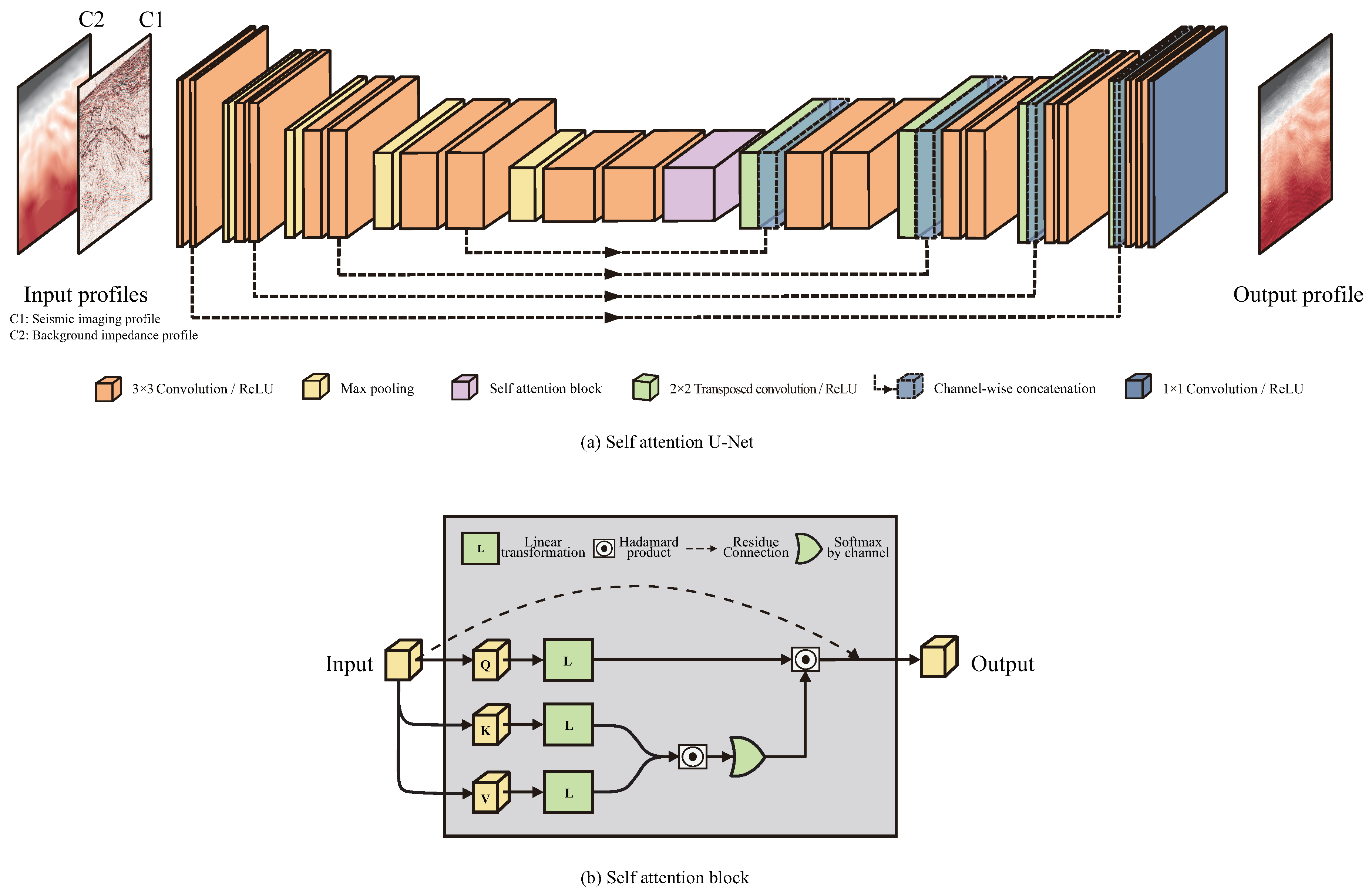
Figure 1.
Architecture of Self attention U-Net.
Figure 1.
Architecture of Self attention U-Net.
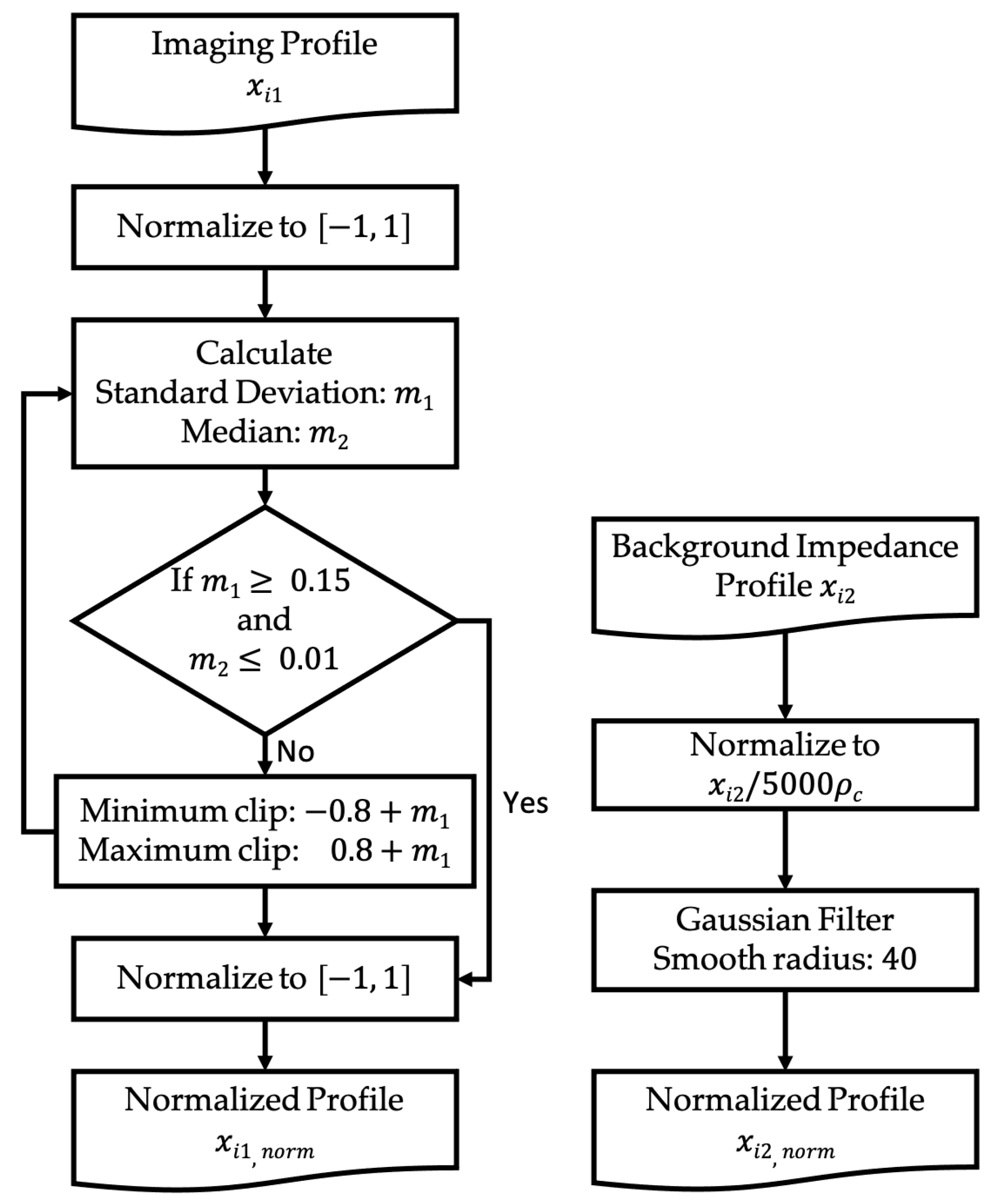
Figure 2.
Workflow of pre-process strategy.
Figure 2.
Workflow of pre-process strategy.
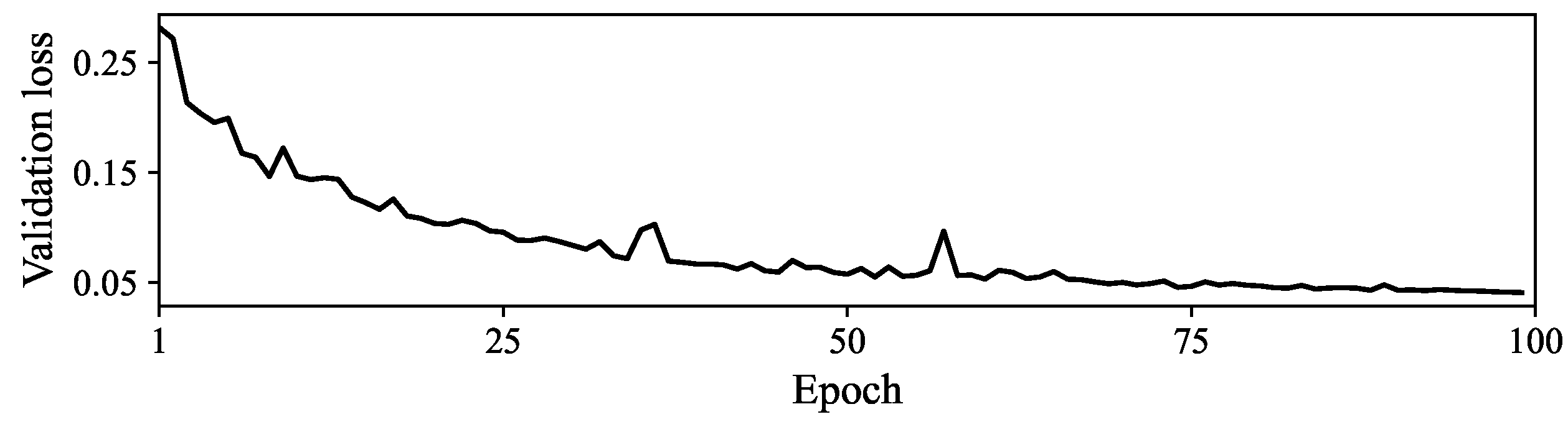
Figure 3.
Loss curve during validation.
Figure 3.
Loss curve during validation.
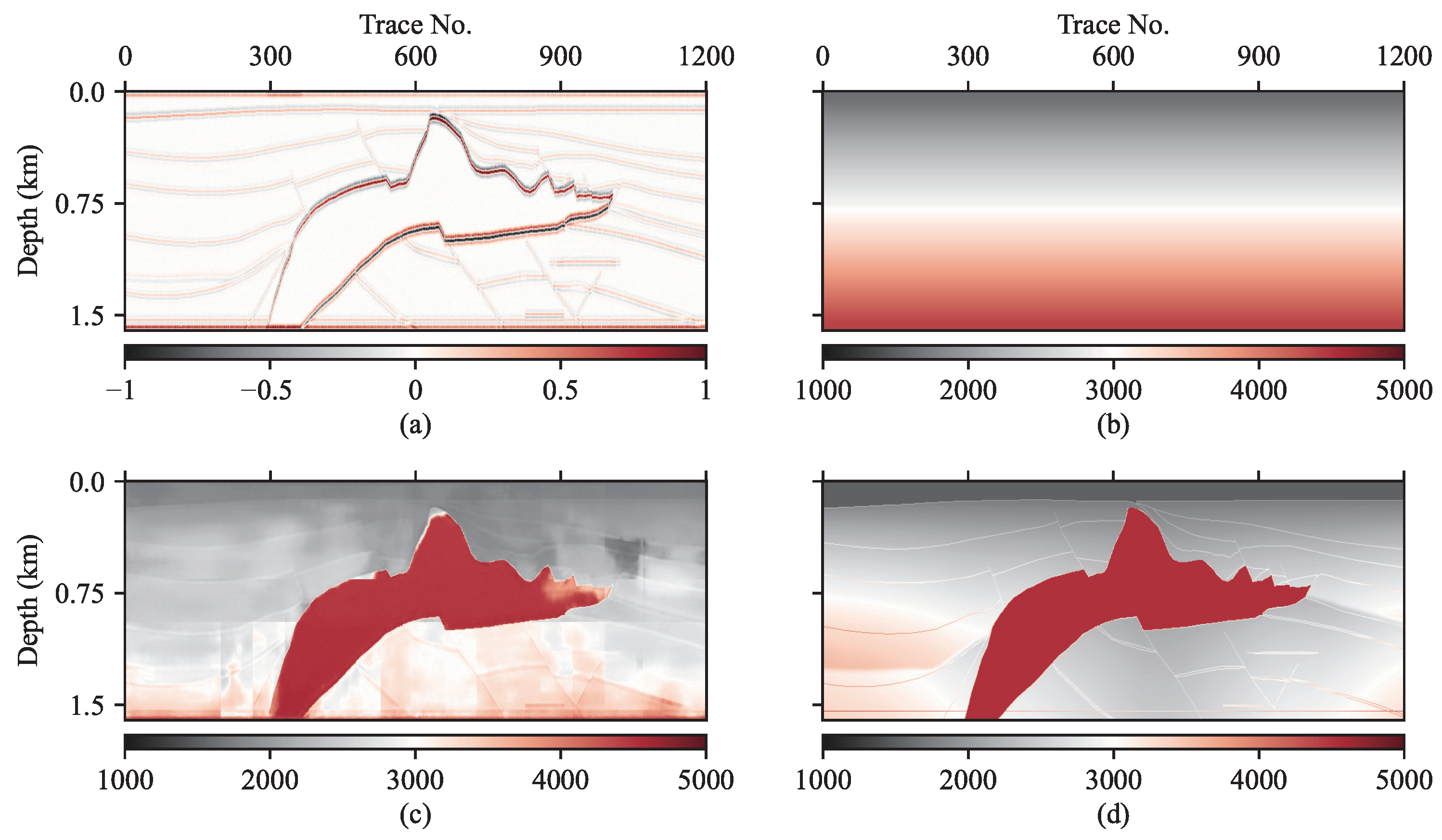
Figure 4.
Inversion of the SEG/EAGE Salt model based on 1D linear background impedance profile: (a) channel 1 of input: imaging profile, (b) channel 2 of input: background impedance profile, (c) inversion by proposed method, (d) original salt model.
Figure 4.
Inversion of the SEG/EAGE Salt model based on 1D linear background impedance profile: (a) channel 1 of input: imaging profile, (b) channel 2 of input: background impedance profile, (c) inversion by proposed method, (d) original salt model.
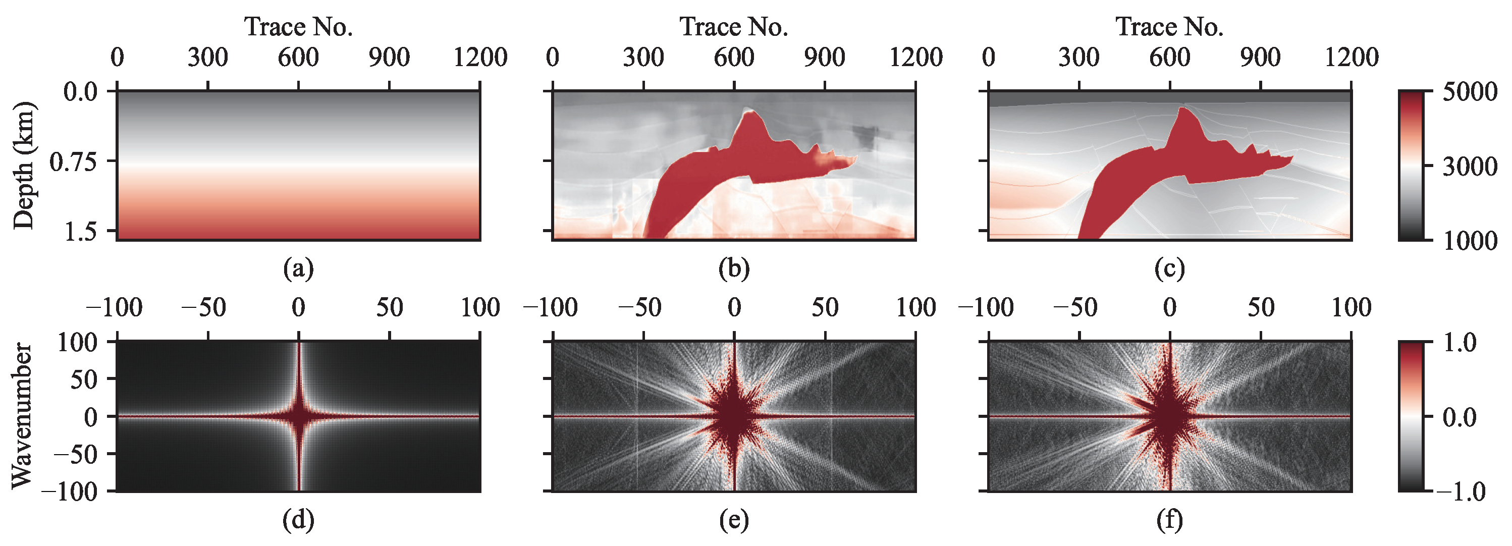
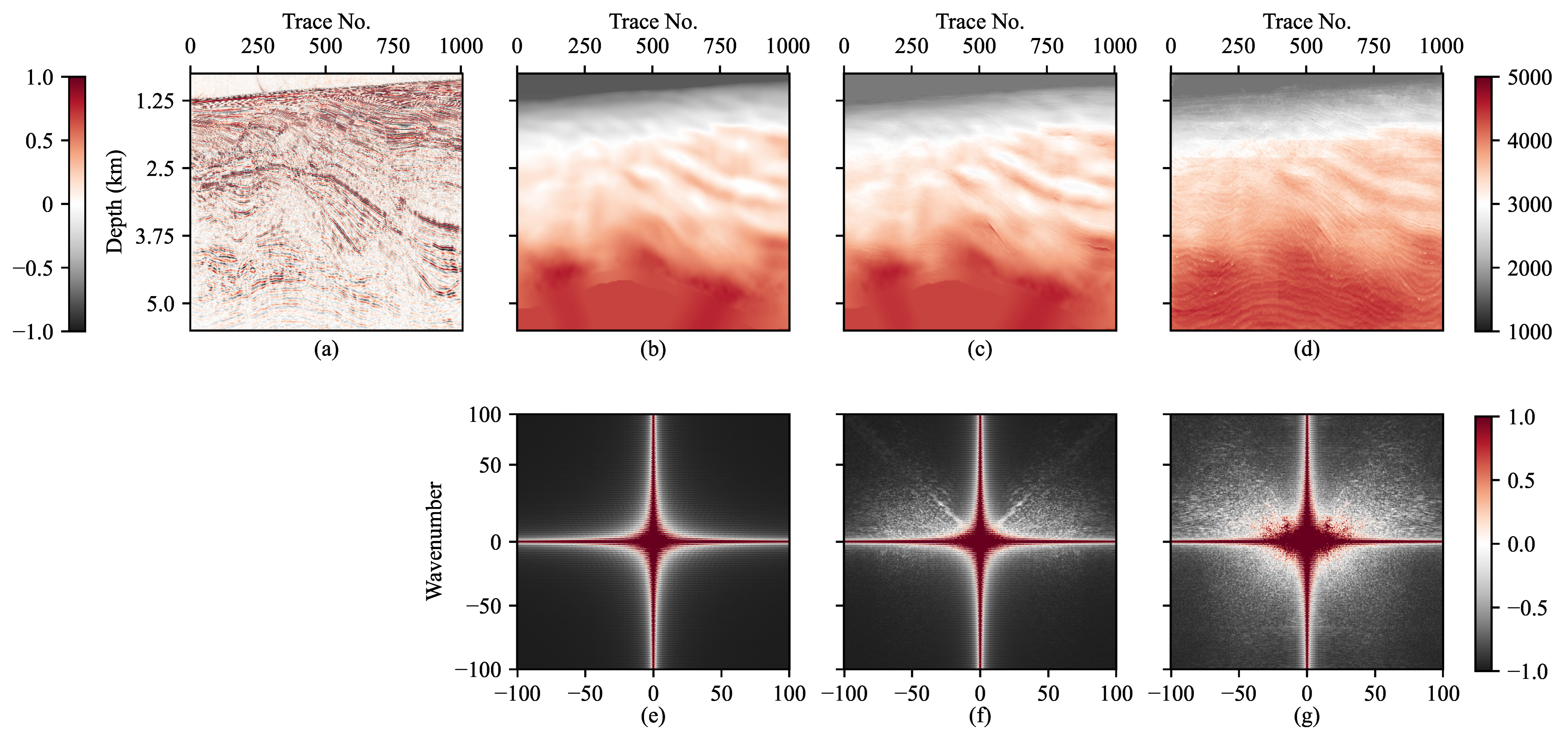
Figure 5.
Inversion and wavenumber spectra of the SEG/EAGE Salt model based on 1D linear background impedance profile: (a) background impedance profile, (b) inversion by proposed method, (c) salt model, (d–f) are corresponding wavenumber spectra to (a–c).
Figure 5.
Inversion and wavenumber spectra of the SEG/EAGE Salt model based on 1D linear background impedance profile: (a) background impedance profile, (b) inversion by proposed method, (c) salt model, (d–f) are corresponding wavenumber spectra to (a–c).
Figure 6.
Inversion of the Marmousi model based on 1D linear background impedance profile, (a) imaging profile: (b) background impedance profile, (c) inversion by proposed method, (d) original Marmousi model.
Figure 6.
Inversion of the Marmousi model based on 1D linear background impedance profile, (a) imaging profile: (b) background impedance profile, (c) inversion by proposed method, (d) original Marmousi model.
Figure 7.
Inversion of the SEG/EAGE Salt model based on 1D logging background impedance profile without high impedance: (a) imaging profile, (b) background impedance profile, (c) inversion by the proposed method, (d) original salt model and location of logging trace marked by dotted line is No. 1050.
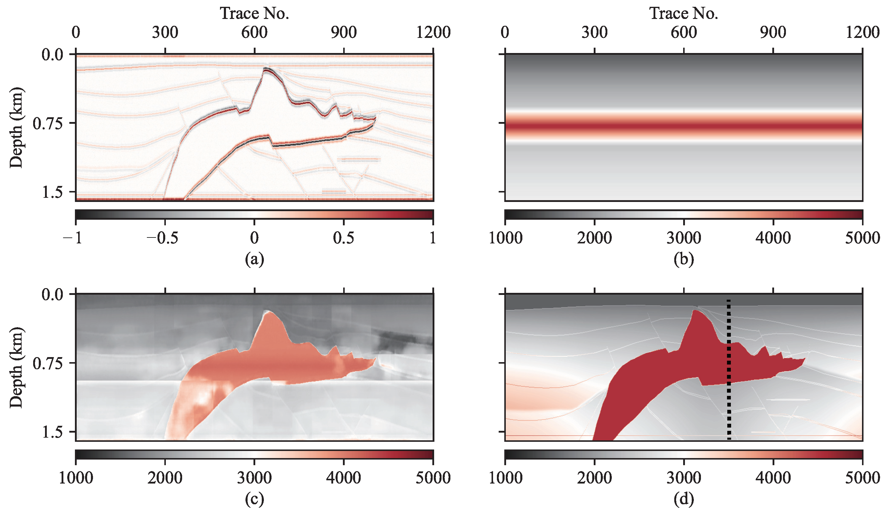
Figure 8.
Inversion and wavenumber spectra of the SEG/EAGE Salt model based on 1D logging background impedance profile with high impedance: (a) imaging profile, (b) background impedance profile, (c) inversion by the proposed method, (d) original salt model and location of logging trace marked by dotted line is No. 750.
Figure 9.
Inversion of the Marmousi model based on 1D logging background impedance profile with high impedance: (a) imaging profile, (b) background impedance profile, (c) inversion by proposed method, (d) original Marmousi model.
Figure 9.
Inversion of the Marmousi model based on 1D logging background impedance profile with high impedance: (a) imaging profile, (b) background impedance profile, (c) inversion by proposed method, (d) original Marmousi model.
Figure 10.
Inversion of the SEG/EAGE Salt model based on 2D Gaussian-blurred background impedance profile: (a) imaging profile, (b) background impedance profile, (c) inversion by the proposed method, (d) original salt model.
Figure 10.
Inversion of the SEG/EAGE Salt model based on 2D Gaussian-blurred background impedance profile: (a) imaging profile, (b) background impedance profile, (c) inversion by the proposed method, (d) original salt model.
Figure 11.
Inversion of the Marmousi model based on 2D Gaussian-blurred background impedance profile: (a) imaging profile, (b) background impedance profile, (c) inversion by the proposed method, (d) original Marmousi model.
Figure 11.
Inversion of the Marmousi model based on 2D Gaussian-blurred background impedance profile: (a) imaging profile, (b) background impedance profile, (c) inversion by the proposed method, (d) original Marmousi model.
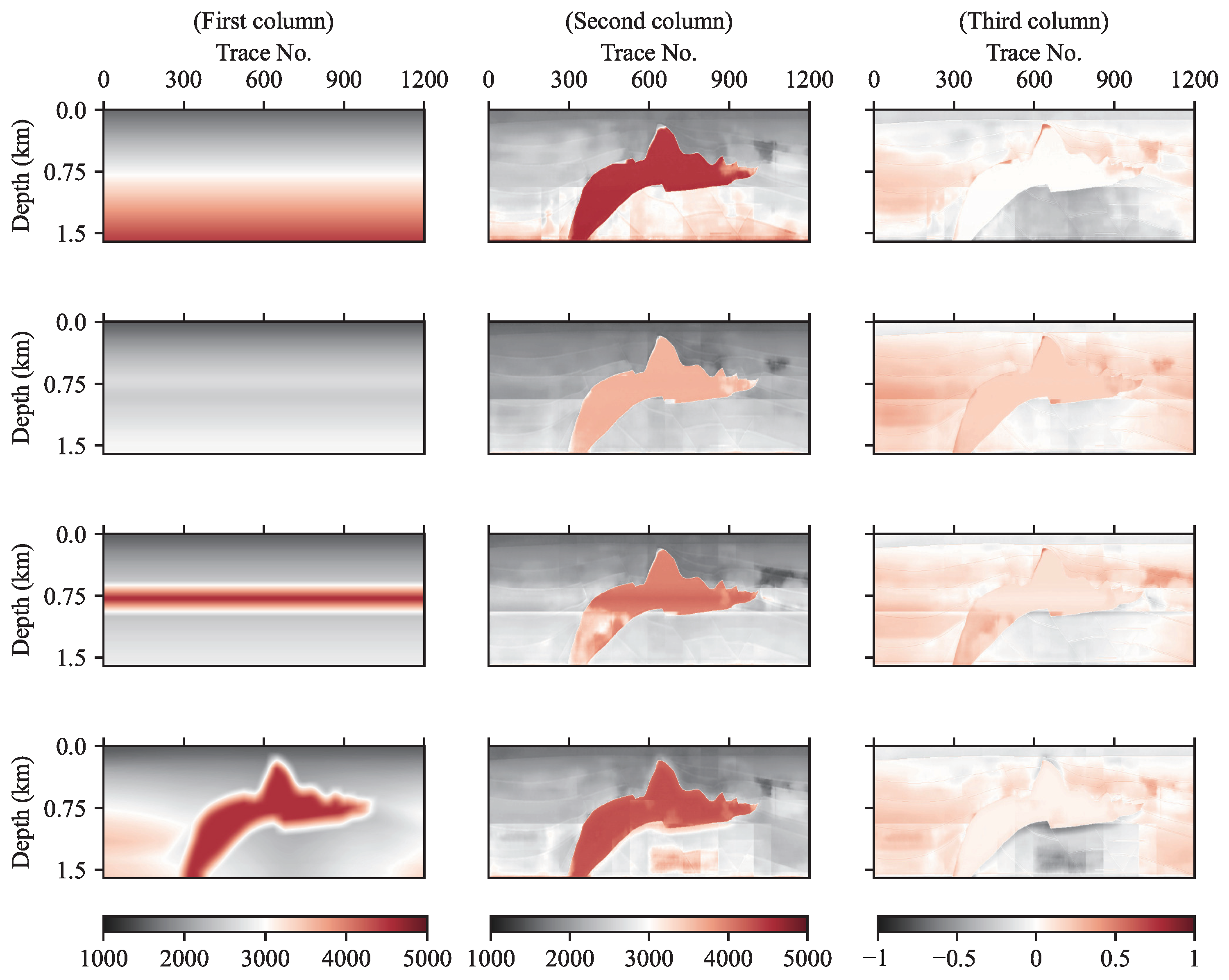
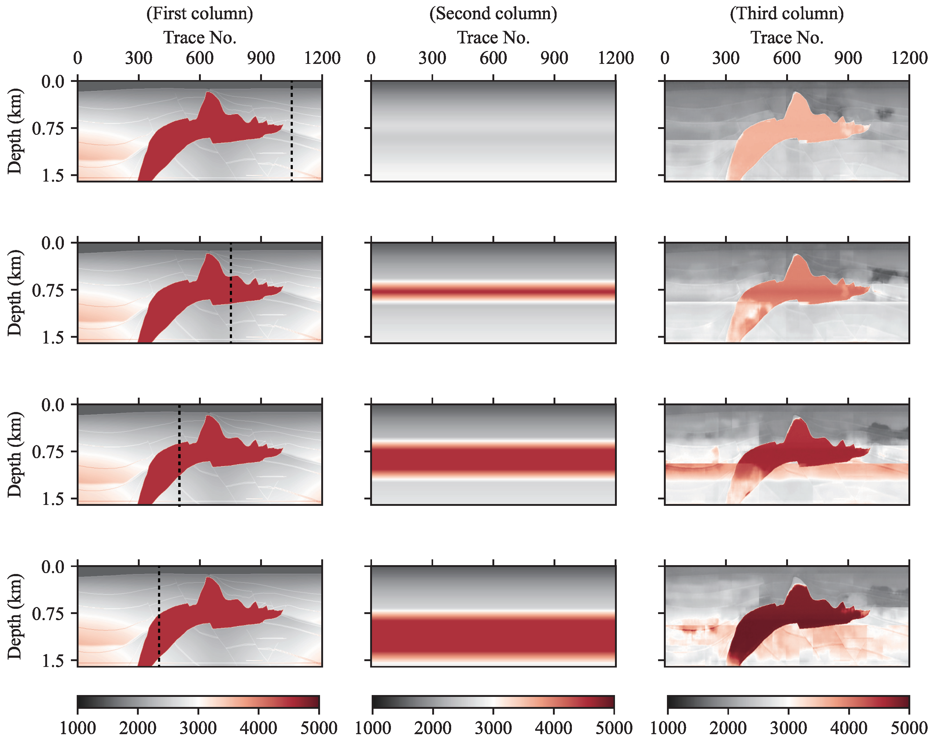
Figure 12.
Relative errors between the SEG/EAGE Salt model and inversions which are inverted by four types of background impedance profiles: (first column) 1D linear, 1D logging without, with high impedance, and 2D Gaussian-blurred background impedance profiles; (second column) inversions; (third column) relative errors between the true model and inversions in the second column.
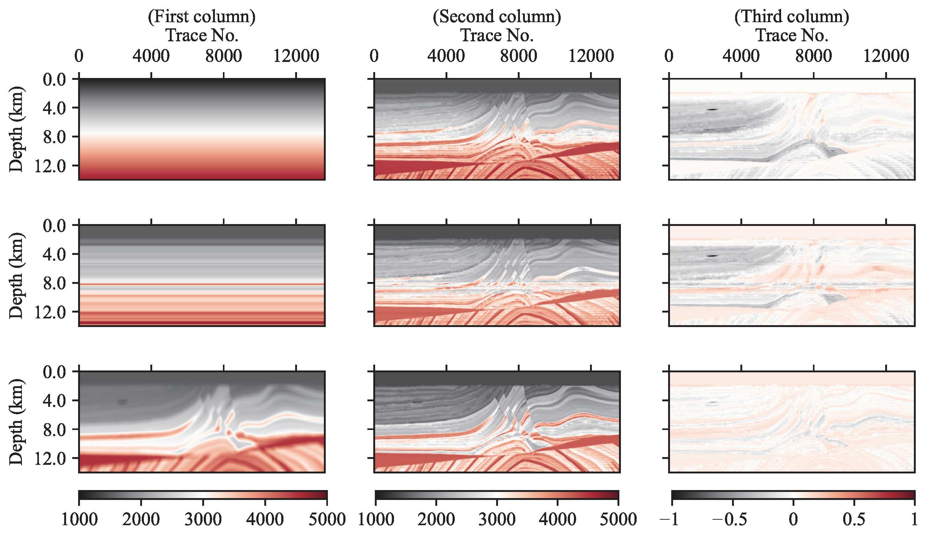
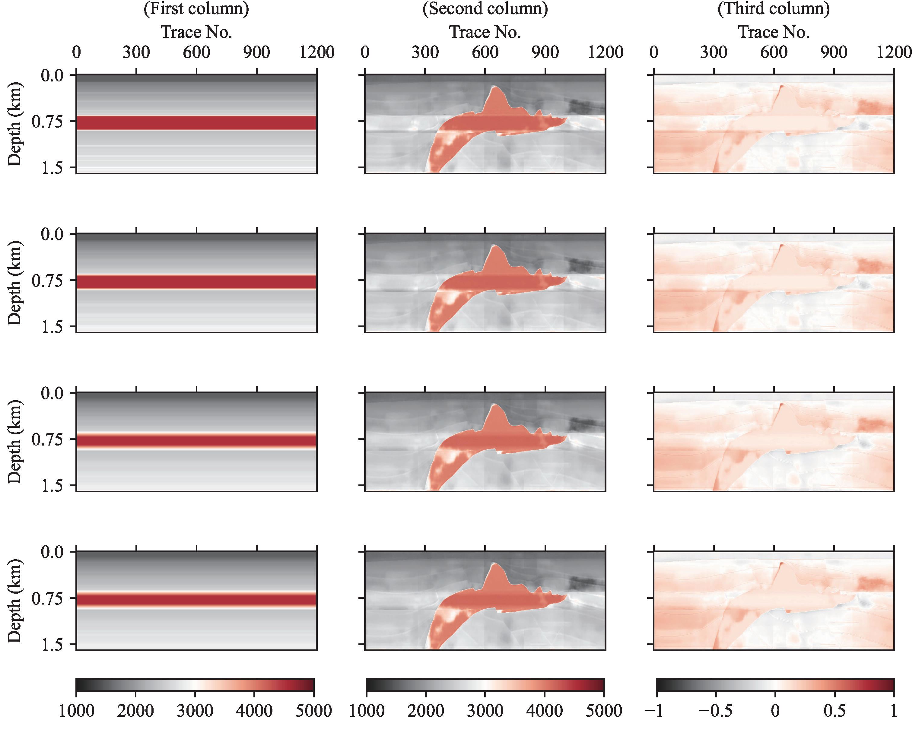
Figure 13.
Relative errors between the Marmousi model and inversions which are inverted by three types of background impedance profiles: (first column) 1D linear, 1D logging, and 2D Gaussian-blurred background impedance profiles; (second column) inversions; (third column) relative errors between the true model and inversions in the second column.
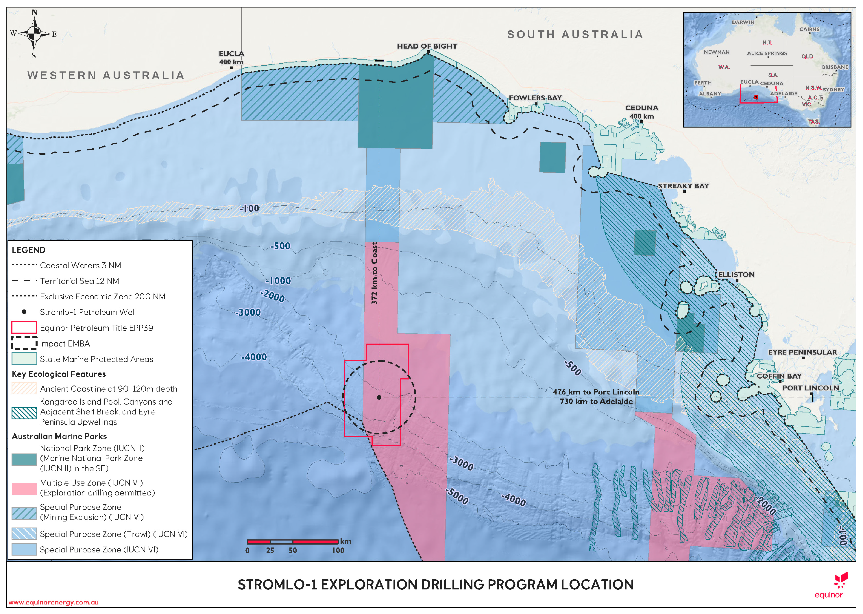
Figure 14.
The location of
Ceduna sub-basin survey area [
40].
Figure 14.
The location of
Ceduna sub-basin survey area [
40].
Figure 15.
Inversion based on Ceduna sub-basin marine seismic data: (a) RTM profile (inline No. 550) after pre-process, (b) migration velocity profile as a background impedance profile with constant density in this research, (c) inversion by the previous strategy where pre-process and iteration in test stage are not contained, (d) inversion by the proposed strategy, (e–g) are corresponding wavenumber spectra of (b–d).
Figure 16.
Inversions with different widths of high-impedance layers based on different logging traces (first column) Salt model and locations of logging traces marked by black lines are No. 1050, 750, 500, and 400 from top to bottom (second column). One-dimensional logging background profiles with different widths of high-impedance layers (third column) inversions based on the second column.
Figure 17.
Inversions with and without pre-process on imaging profile. (a,b) RTM imaging profile with pre-process and inversion, (c,d) RTM imaging profile without pre-process and inversion.
Figure 17.
Inversions with and without pre-process on imaging profile. (a,b) RTM imaging profile with pre-process and inversion, (c,d) RTM imaging profile without pre-process and inversion.
Figure 18.
Inversions by different background impedance profiles with smoothing radius. (First column) background profiles with different blurred radii, from top to bottom, are 5, 10, 20, and 40 grids, respectively; (second column) corresponding inversions; and (third column) relative errors.
Figure 18.
Inversions by different background impedance profiles with smoothing radius. (First column) background profiles with different blurred radii, from top to bottom, are 5, 10, 20, and 40 grids, respectively; (second column) corresponding inversions; and (third column) relative errors.
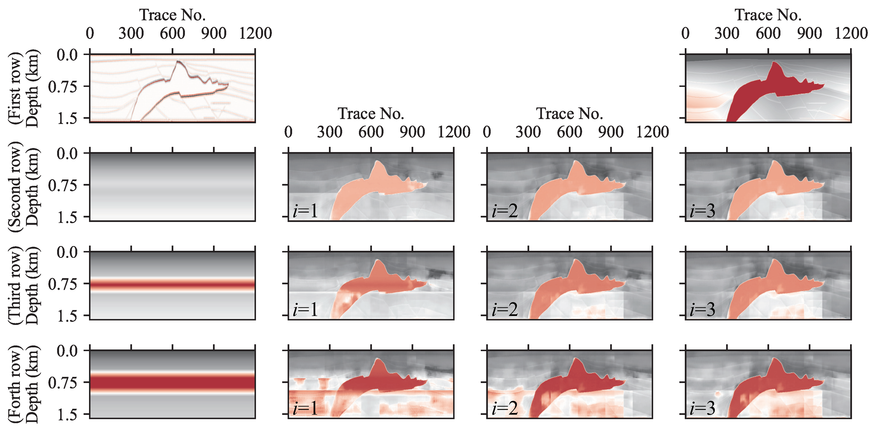
Figure 19.
Inversions of RTM data based on different widths of high-impedance layers by three-times iterations. (First row) input including RTM profile and the SEG/EAGE Salt model, (second row) background profile without high impedance and inversions at iteration 1, 2, 3, (third row) background profile with high impedance layer and inversions at iteration 1, 2, 3, (second row) background profile with wider high impedance layer and inversions at iteration 1, 2, 3.
Table 1.
Architecture of U-Net.
Table 1.
Architecture of U-Net.
| Layer | Input (BS, W, H, C) | Type | Output (BS, W, H, C) |
|---|
| 1 | (1, 200, 200, 2) | Input | (1, 200, 200, 64) |
| 2 | (1, 200, 200, 64) | Forward convolution | (1, 100, 100, 128) |
| 3 | (1, 100, 100, 128) | Forward convolution | (1, 50, 50, 256) |
| 4 | (1, 50, 50, 256) | Forward convolution | (1, 25, 25, 512) |
| 5 | (1, 25, 25, 512) | Forward convolution | (1, 12, 12, 1024) |
| 6 | (1, 12, 12, 1024) | Self attention | (1, 12, 12, 1024) |
| 7 | (1, 12, 12, 1024) | Transposed convolution | (1, 25, 25, 512) |
| 8 | (1, 25, 25, 512) | Transposed convolution | (1, 50, 50, 256) |
| 9 | (1, 50, 50, 256) | Transposed convolution | (1, 100, 100, 128) |
| 10 | (1, 100, 100, 128) | Transposed convolution | (1, 200, 200, 64) |
| 11 | (1, 200, 200, 64) | Output | (1, 200, 200, 1) |
Table 2.
Details of layers.
Table 2.
Details of layers.
| Type | Input shape | Operation | Activation | Channel | Filter | Strid | Padding | Output |
|---|
| Input | (BS, NVX, NVZ, 2) | Convolution | ReLU | 64 | 3 × 3 | 1 | Same | (BS, NVX, NVZ, 64) |
| Forward convolution | (BS, W, H, C) | Convolution | ReLU | C | 3 × 3 | 1 | Same | (BS, W, H, C) |
| | (BS, W, H, C) | Max pool | - | - | 2 × 2 | 2 | - | (BS, W/2, H/2, C) |
| | (BS, W/2, H/2, C) | Convolution | ReLU | 2C | 3 × 3 | 1 | Same | (BS, W/2, H/2, 2C) |
| Self attention | (BS, W, H, C) | Convolution | Softmax | 1 | 1 × 1 | 1 | Same | (BS, W, H, C) |
| Transposed convolution | (BS, W/2, H/2, 2C) | Convolution | ReLU | C | 2 × 2 | 2 | Same | (BS, W, H, C) |
| | (BS, W, H, C) | Channel-wise concatenation | - | C+C | - | - | Same | (BS, W, H, 2C) |
| | (BS, W, H, 2C) | Convolution | ReLU | C | 3 × 3 | 1 | Same | (BS, W, H, C) |
| | (BS, W, H, C) | Convolution | ReLU | C | 3 × 3 | 1 | Same | (BS, W, H, C) |
| Output | (BS, NVX, NVZ, 64) | Convolution | ReLU | 1 | 3 × 3 | 1 | Same | (BS, NVX, NVZ, 1) |
Table 3.
Notes of testing data.
Table 3.
Notes of testing data.
| Model | Type of Imaging Profiles | Type of Background Impedance Profiles |
|---|
| SEG/EAGE Salt | | 1D linear |
| and Marmousi | Synthetic | 1D logging |
| | | 2D Gaussian-blurred |
| Ceduna sub-basin | RTM | Migration velocity with constant density |
Table 4.
MSE.
| First Column | Second Column |
|---|
| 1.0946 | 0.2031 |
| 0.8790 | 0.1561 |
| 0.7728 | 0.1426 |
| 0.1901 | 0.0838 |
Table 5.
MSE.
| First Column | Second Column |
|---|
| 0.2447 | 0.0892 |
| 0.3332 | 0.1085 |
| 0.0295 | 0.0148 |
Table 6.
MSE.
| Second Column | Third Column |
|---|
| 0.8790 | 0.1561 |
| 0.7728 | 0.1426 |
| 0.8258 | 0.2491 |
| 1.0000 | 0.2057 |
Table 7.
MSE.
| (a) | (b) | (c) | (d) |
|---|
| 0.8782 | 0.3999 | 0.8584 | 0.7821 |
Table 8.
MSE.
| First Column | Second Column |
|---|
| 0.8783 | 0.1309 |
| 0.8584 | 0.1299 |
| 0.8266 | 0.1290 |
| 0.7728 | 0.1291 |


