Article

PJ-YOLO: Prior-Knowledge and Joint-Feature-Extraction Based YOLO for Infrared Ship Detection

Institute of Logistics Science and Engineering, Shanghai Maritime University, Shanghai 201306, China
*
Authors to whom correspondence should be addressed.
J. Mar. Sci. Eng. 2025, 13(2), 226; https://doi.org/10.3390/jmse13020226
Submission received: 25 December 2024 / Revised: 17 January 2025 / Accepted: 22 January 2025 / Published: 25 January 2025
(This article belongs to the Section Ocean Engineering)

Abstract

:
Infrared ship images have low resolution and limited recognizable features, especially for small targets, leading to low accuracy and poor generalization of traditional detection methods. To address this, we design a prior knowledge auxiliary loss for leveraging the unique brightness distribution of infrared ship images, we construct a joint feature extraction module that sufficiently captures context awareness, channel differentiation, and global information, and then we propose a prior-knowledge- and joint-feature-extraction-based YOLO (PJ-YOLO) for use in detecting infrared ships. Additionally, a residual deformable attention module is designed to integrate multi-scale information, enhancing detail capture. Experimental results on the SFISD and InfiRray Ships datasets demonstrate that the proposed PJ-YOLO achieves state-of-the-art detection performance for infrared ship targets. In particular, PJ-YOLO achieves improvements of 1.6%, 5.0%, and 2.8% in mAP50, mAP75, and mAP50:95 on the SFISD dataset, respectively.

1. Introduction

The safety of maritime navigation is threatened by numerous risk factors, including adverse weather conditions, navigational obstacles, and technical malfunctions, among others. The rapid development of the global shipping industry, coupled with the rise of unmanned surface ships and intelligent industries, has increased the number and variety of ships, making maritime navigation safety more complex [1]. To better mitigate accident risks, ensure navigation safety, and enhance the efficiency of maritime traffic management, effective and accurate detection of ships has become a key research field.
In recent years, with the advancement of infrared technology, infrared object detection has gradually become a research focus. Infrared images, formed by capturing the infrared radiation of objects, possess advantages that are irreplaceable by visible images. These advantages include all-weather capabilities and strong adaptability to complex environments, addressing the limitations of visible images, which are susceptible to environmental factors and struggle with imaging under low-light conditions [2]. Infrared imaging finds widespread applications in various fields such as military, agriculture, medicine and transportation.
Traditional infrared object detection methods include wavelet transform [3], template matching [4], and contrast mechanism-based methods [5], among others. However, these methods have limited accuracy, as they rely on manually designed features. Domain expertise and experience are required to manually select and design features for representing targets. These features often struggle to capture advanced semantic information on complex targets, resulting in poor generalization and limited adaptability to changes in target size. This inadequacy hinders their ability to effectively meet the requirements of ship detection tasks.
The rapid development of deep learning technology has led to powerful feature extraction capabilities, significantly outperforming traditional algorithms in detection performance. This advancement has been widely applied across various fields, such as semantic segmentation [6], keypoint detection [7], and image dehazing [8], further demonstrating its versatility and effectiveness in tackling complex tasks. Convolutional neural network (CNN)-based object detection algorithms excel at automatically learning hierarchical feature representations from raw pixel data, which enables them to detect and localize objects with high accuracy and robustness. Compared to traditional methods, which rely on manually designed features, CNNs can automatically learn and extract complex and abstract features, thereby overcoming the limitations of these methods.
For ship detection, Wen et al. [9] proposed a multi-scale, single-shot detector (MS-SSD) and introduced a scale-aware scheme, which demonstrated excellent performance for small targets while performing less effectively for larger ones. Zhan et al. [10] proposed an edge-guided structure-based object detection network named EGISD-YOLO for infrared ship detection. Li et al. [11] designed a complete YOLO-based ship detection method (CYSDM) for thermal infrared remote sensing ship detection in complex backgrounds, providing a reference for large-scale and all-weather ship detection. Yuan et al. [12] proposed a multitype feature perception and refined network (MFPRN) combining a fast Fourier module and a lightweight multilayer perceptron. This method effectively reduces false detections, but it has a large number of parameters and high computational costs. Although these methods have innovated feature extraction and designed detectors suitable for ship detection, they primarily focus on extracting features from the images without fully utilizing the inherent characteristics of the targets. For example, information such as the shape, motion patterns, and thermal radiation characteristics of the ships is not adequately considered, leading to missed and false detections.
CNN-based detection algorithms have made certain progress in the task of infrared ship detection, but there are still some challenges that need to be overcome. Ship targets in infrared images often exhibit weak features, especially small ones, lacking clear shapes and texture details. The limited recognizable features contribute to increased uncertainty in detection results. Therefore, it is necessary to enhance the extraction of these limited features. Additionally, ships vary greatly in size and have irregular shapes, further limiting the robustness of infrared ship detection. Moreover, the intrinsic characteristics of ship targets can be fully incorporated, enabling more precise and reliable feature extraction tailored to the unique traits of these objects. To address the aforementioned challenges, this paper proposes the PJ-YOLO, which uses YOLOv8 [13] as the baseline. The main contributions of this paper are as follows:
(1)
We propose a novel PJ-YOLO network for infrared ship detection. It integrates prior knowledge auxiliary loss, which leverages the unique brightness distribution characteristics between ships and backgrounds in infrared images as prior knowledge, and also incorporates a joint feature extraction module and a residual deformable attention module.
(2)
To address the challenge of weak and elusive features in infrared images, particularly for small ship targets, we construct a joint feature extraction module to enhance feature extraction ability by utilizing channel-differentiated features, context-aware information, and global information. This module effectively captures subtle characteristics of ship targets.
(3)
Considering the multiscale nature of ship targets, a residual deformable attention module is designed within the higher layers of the backbone network, which effectively integrates multi-scale information to significantly enhance detail capture and improve detection performance.
The remainder of this paper is organized as follows: Section 2 reviews related works. Section 3 describes the overall framework of PJ-YOLO and its modules. Section 4 presents comparative experiments and analyses on the infrared ship datasets. Finally, Section 5 provides the conclusion.

2. Related Work

2.1. Deep Learning-Based Schemes

Deep learning-based object detection methods can be divided into CNN-based methods and transformer-based methods.
CNN-based methods primarily rely on convolution operations to extract features, gradually building an understanding of the image, and can further be categorized into two-stage and one-stage approaches. Two-stage approaches first generate region proposals and then perform further classification and bounding box regression on these proposals. Representative algorithms such as Fast R-CNN [14], Faster R-CNN [15], and Cascade R-CNN [16] have been widely used in object detection tasks. One-stage approaches extract features using CNNs and simultaneously predict the classification and localization of targets, eliminating the step of generating region proposals. Typical algorithms in this category include SSD [17], RetinaNet [18], and YOLO [19]. YOLO, in particular, is renowned for its excellent real-time performance and low computational cost, making it well-suited for real-time applications or scenarios with high speed requirements. For instance, YOLOv8 and YOLOv9 [20] continue the excellent tradition of the YOLO series while introducing advanced techniques and innovations. YOLOv8 adopts a new C2f structure in the backbone network, providing richer gradient flow and employing an anchor-free design. YOLOv9 adopts a lightweight architecture and introduces programmable gradient information, using reversible branches to preserve key deep features for effective object detection. However, for infrared ship detection tasks, these YOLO-like methods still confront significant challenges. Infrared images are characterized by weak and elusive features as well as the presence of numerous small targets that are prone to being missed, which collectively make target detection inherently more difficult. The performance of existing YOLO-like methods remains limited, often resulting in issues such as missed detections and false alarms.
Transformer-based methods leverage the self-attention mechanism to capture global contextual information within images, and RT-DETR [21] is a representative of such approaches. Transformer-based methods excel at capturing global features and long-range dependencies, but they are resource-intensive, slower to train, and often require large datasets for effective performance. By comparison, modern CNN-based methods are generally more suitable for real-time detection tasks.

2.2. Knowledge-Driven Infrared Object Detection

In object detection, “prior knowledge” refers to pre-existing or previously acquired information or assumptions about the target that can help the algorithm better understand and locate it. This prior knowledge can encompass information regarding the target’s size, brightness, shape, appearance characteristics, and spatial distribution.
Prior knowledge plays a crucial role in infrared object detection by leveraging prior understanding of target features and background information, thereby enhancing detection accuracy. Zhu et al. [22] combined the structural prior knowledge of infrared small targets with the autocorrelation of the background to propose infrared small target detection based on low-rank tensor completion and ring top-hat regularization. Liu et al. [23] proposed an infrared object detection algorithm that combines low-rank prior with deep denoising prior. Gao et al. [24] proposed an infrared cirrus cloud detection model based on multi-directional graph learning and local fractal feature prior weight mapping. This model improves the low-rank characteristics and smoothness of the background, resulting in more complete detection of cirrus cloud structures. Zhang et al. [25] proposed a prior model based on the assumption that infrared targets are locally prominent. This model serves as a constraint for the target tensor, effectively reducing the false detection of sparse edge structures. However, existing methods are typically optimized for targets of specific scales, making it difficult to effectively handle multi-scale targets, especially when the target size varies significantly. Additionally, their generalization capability is limited, as they are often designed for specific scenarios and may not perform well in diverse or complex environments.

2.3. Data-Driven Infrared Object Detection

The data-driven approach refers to the methodology of training models with large amounts of annotated data, enabling them to learn and understand the features and contextual information of targets from the data, thereby achieving automated target recognition and localization.
Data-driven deep learning methods have achieved significant application success in various tasks of infrared object detection. To address the challenges posed by the complexity of the background and occlusion among multiple targets, Xu et al. [26] proposed a contour information-guided multiscale feature detection method to enhance the accuracy of pedestrian target detection. Du et al. [27] incorporated the YOLOv4 model into the context of detecting weakly visible and severely occluded vehicles in infrared aerial images amid complex backgrounds. Nonetheless, their method depends on K-means clustering for anchor box determination, necessitating extensive hyperparameter adjustment. To address the challenge of accuracy loss due to the absence of texture features in infrared objects, Bao et al. [28] proposed the Dual-YOLO incorporating attention fusion and shuffle design to achieve simplified and effective fusion of information. However, this solution substantially increases computational demands. To accurately and swiftly detect infrared long-range aerial targets in complex backgrounds, Jiang et al. [29] presented a lightweight multiscale infrared aircraft recognition algorithm. They used a focus module to reduce computational load and a Res2net-based feature extraction design to improve accuracy. Nevertheless, their approach is prone to missed detections. Bhat Kera et al. [30] explored a domain adaptation approach and designed a staged block-wise framework to repurpose the EfficientDet object detector for operation in the thermal infrared domain. Despite its effectiveness, the method faces challenges in managing occlusion scenarios. Zhou et al. [31] integrated existing convolutional backbones with the contemporary transformer architecture to develop a novel combined backbone model named IRMultiFuseNet for infrared ship detection. While the methods outlined above primarily focus on model design, it is also important to consider the inherent characteristics of different types of infrared targets, which could further improve detection performance.

3. Proposed Method

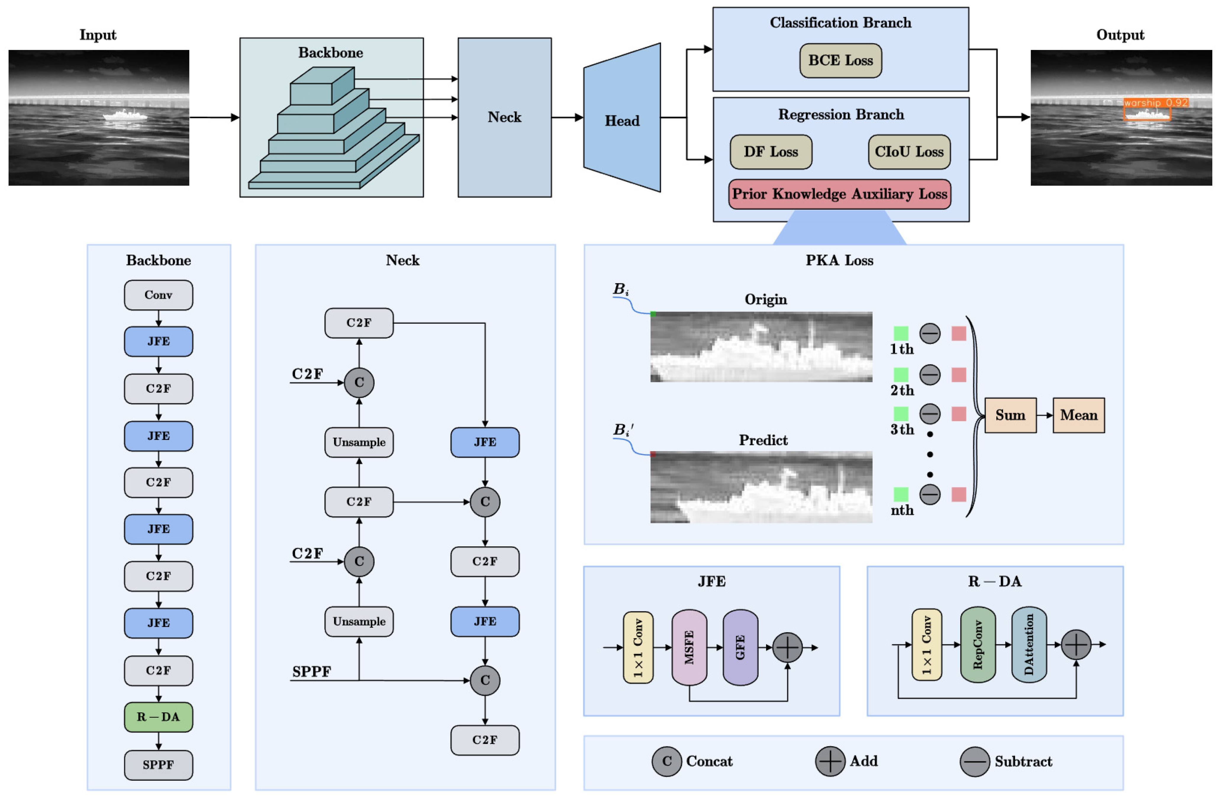
The overall architecture of the proposed PJ-YOLO is shown in Figure 1. In this network, the backbone and neck parts incorporate the joint feature extraction (JFE) module, which enhances feature extraction from multiple dimensions by integrating channel-differentiated features, context-aware information, and global information. This module is particularly effective in capturing subtle characteristics of ship targets, especially in scenarios with weak features or small targets. To better integrate multi-scale information, a residual deformable attention (R-DA) module is introduced in the high layers of the backbone, improving the model’s robustness to scale variations and complex backgrounds. Additionally, considering the significant brightness difference between ships and their backgrounds, an infrared ship prior knowledge auxiliary loss is designed. This loss function utilizes the prior knowledge of brightness distribution differences to guide the network in accurately locating targets, effectively reducing false alarms and missed detections. By combining the JFE module, R-DA module, and prior knowledge auxiliary loss, PJ-YOLO achieves an optimal balance between accuracy and speed, demonstrating strong potential for practical applications in infrared ship detection tasks.

3.1. Joint Feature Extraction Module

In infrared ship images, the available target features are limited, and it is particularly difficult to identify and obtain relevant features for small infrared targets. Therefore, a joint feature extraction (JFE) module has been designed to enhance feature extraction capability across multiple dimensions, including channel, context-aware, and global information. The structure of the JFE module is shown in Figure 2. The number of channels in the feature map is adjusted through a 1 × 1 convolution followed by multi-scale and global feature extraction using Multi-Scale Feature Extractor (MSFE) and Global Feature Extractor (GFE), respectively, with subsequent feature fusion. The residual connection designed after the MSFE facilitates the flow of information between network layers.
The MSFE consists of two branches, each designed to enhance the network’s focus on differentiated features and better capture context-aware information. The first branch is implemented with Self-Calibrated Convolution (SCConv) [32]. Similar to regular convolutions, SCConv separates each channel of the convolution. However, SCConv channels are responsible for specific functions or information. Through dual mapping in the original scale space features and the downsampling latent space features, the network focuses on differentiated features, enhancing channel feature extraction capabilities. The second branch is achieved through three dilated convolutions with different dilation rates. By introducing dilation into the convolutional kernels, the receptive field is expanded, allowing for better capture of context information and strengthening the extraction of spatial features. Compared to regular convolutions, dilated convolutions maintain the same receptive field size while reducing the number of parameters and computational load. Finally, the features extracted from both branches are fused. This process can be expressed as follows:
MSFE ( x ) = ReLU BN Concat SCConv ( x ) , DConv 1 ( x ) , DConv 3 ( x ) , DConv 5 ( x ) ,
where x is the input feature, and D C o n v 1 , D C o n v 3 , and D C o n v 5 represent dilated convolutions with dilated coefficients of 1, 3, and 5, respectively.
The GFE first processes the input by applying ReLU activation subsequent to both global max-pooling and global average-pooling operations. Global max-pooling captures the most prominent features by selecting the maximum value from each feature map, effectively highlighting the most significant characteristics of the image. In contrast, global average-pooling computes the average value of each feature map, maintaining the overall distribution of features and retaining the global context of the image. Finally, the activated features are processed by a fully connected layer, which integrates the salient and global information, thereby guiding the fusion of multi-scale features and improving the overall feature representation. This procedure can be represented as follows:
GFE ( x ) = Sigmoid ( FC ( ReLU ( AvgPool ( x ) ) ) ) + Sigmoid ( FC ( ReLU ( MaxPool ( x ) ) ) ) ,
where x is the input feature.

3.2. Residual Deformable Attention Module

To enhance the model’s focus on objects of varying scales and improve the network’s perception of critical features, an attention module is designed in the high layers of the backbone network. This aims to better capture the features of the targets.
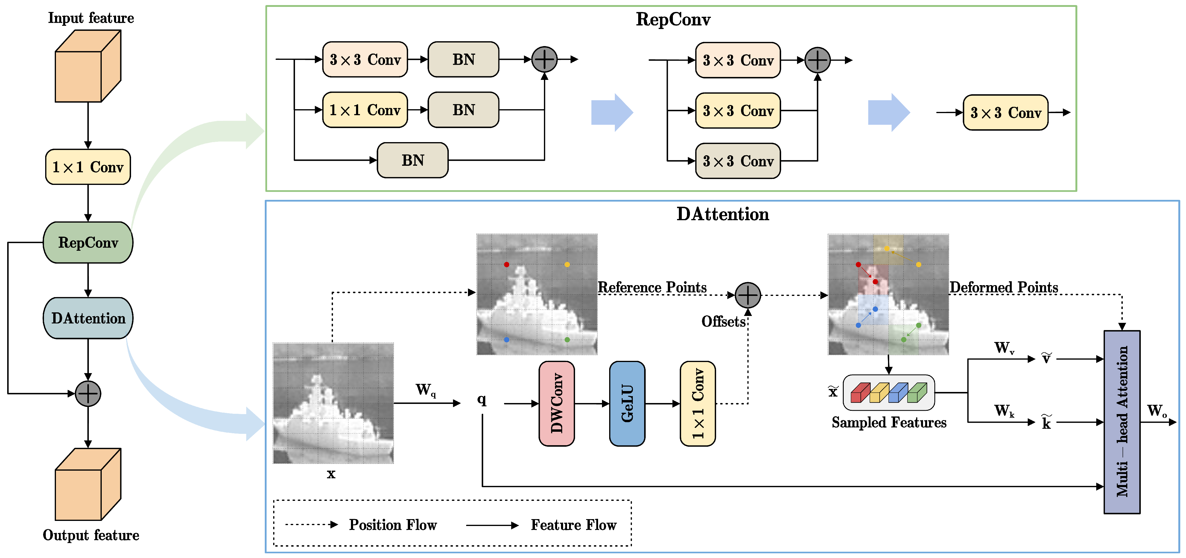
The structure of the residual deformable attention (R-DA) module is shown in Figure 3. The input features first pass through 1 × 1 convolution for cross-channel aggregation. Then, RepConv [33] reparameterization is applied to enhance inference speed without degrading accuracy. Finally, the features pass through DAttention [34], with a residual connection introduced. The inclusion of the residual connection helps retain the original feature information, preventing the loss of important details and semantic information during feature transmission. This makes the network easier to train and addresses potential issues of information loss and gradient vanishing in attention modules. By establishing a connection between the attention module and the residual connection, the network can more accurately learn and utilize key features.
The main motivation of RepConv is to transform as many convolutions as possible into 3 × 3 convolutions, aiming to improve inference speed. As shown in Figure 3, the simplification process of RepConv involves unifying convolutions of different sizes into a single 3 × 3 convolution, followed by an equivalent merging of the batch normalization (BN) parameters into the 3 × 3 convolution. This equivalent merging method converts the mean and variance of BN into the weights and biases of the convolution, allowing for a single convolution operation during inference and thereby improving inference efficiency.
Inspired by deformable convolutions, the DAttention focuses only on a set of key sampling points around a reference point, rather than processing all pixels in the image. This significantly reduces computational overhead while maintaining good performance. Given the input feature map, reference points are generated. To obtain the offset for each reference point, the feature map is linearly projected to the query token. The offset is generated by the offset network, and it is applied to the reference points. In the offset network, the input features are first captured by deep convolution to extract local features. Then, a GeLU activation function and a 1 × 1 convolution are applied to obtain the two-dimensional offset. After obtaining the reference points, local features are captured through bilinear interpolation and used as the input for both key k and value v. Subsequently, the operations of q, k, and v follow the standard self-attention, with an additional relative position offset compensation. The process can be formulated as follows:
q = x W q , k ˜ = x ˜ W k , v ˜ = x ˜ W ν ,
Δ p = θ o f f s e t ( q ) ,
x ˜ = ϕ ( x ; p + Δ p ) ,
where x and x ˜ represent input and sample features, k ˜ and v ˜ represent deformable key embeddings and value embeddings respectively, and ϕ represents bilinear interpolation operation.

3.3. Loss Function

In object detection, the role of the loss function is to guide the optimization process by quantifying the difference between the model’s predictions and the ground truth, with the goal of enabling the model to accurately and robustly detect targets. Regression loss is a crucial component of object detection, as it guides the model in adjusting the predicted bounding boxes during training to more accurately locate the targets. We designed the Prior Knowledge Auxiliary Loss (PKA Loss), incorporating prior knowledge of infrared ships to guide the model in more accurately localizing ship targets based on brightness differences.

3.3.1. Loss Function of the Regression Branch

In vanilla YOLOv8, the regression branch includes the Distribution Focal Loss (DFL) and CIoU Loss functions. The DFL enables the network to quickly focus on the distribution of positions close to the target location, while the CIoU Loss improves upon the IoU Loss by enhancing the precision of the bounding box regression. The DFL is defined as follows:
L D F L i = ( ( y i + 1 y ) l o g S i + ( y y i ) l o g S i + 1 ) ,
where y i and y i + 1 present the values approaching the continuous label y from the left and right sides, and S i represents the Sigmoid output of the i-th branch.
Compared to the IoU loss function, CIoU incorporates considerations of aspect ratio and center point distance in the penalty term. This allows for better adaptation to targets of varying scales and more accurately measures the overlap between the predicted bounding box and the ground truth bounding box. The definition of CIoU is as follows:
I o U = B g t B p r e d B g t B p r e d ,
v = 4 π 2 a r c t a n w g t h g t a r c t a n w h 2 ,
α = v 1 I o U + v ,
L C I o U = 1 I o U + α ν + ρ 2 b , b g t c 2 ,
where B g t denotes ground truth bounding box, B p r e d denotes predicted bounding box, v is used to measure the scale consistency between two bounding boxes, and α is the weighting coefficient. b and b g t are predicted and ground truth bounding box centers, ρ 2 ( · ) represents Euclidean distance between the centers of the two boxes, and c represents the diagonal distance of the smallest enclosing area that can simultaneously contain both boxes.

3.3.2. Prior Knowledge Auxiliary Loss

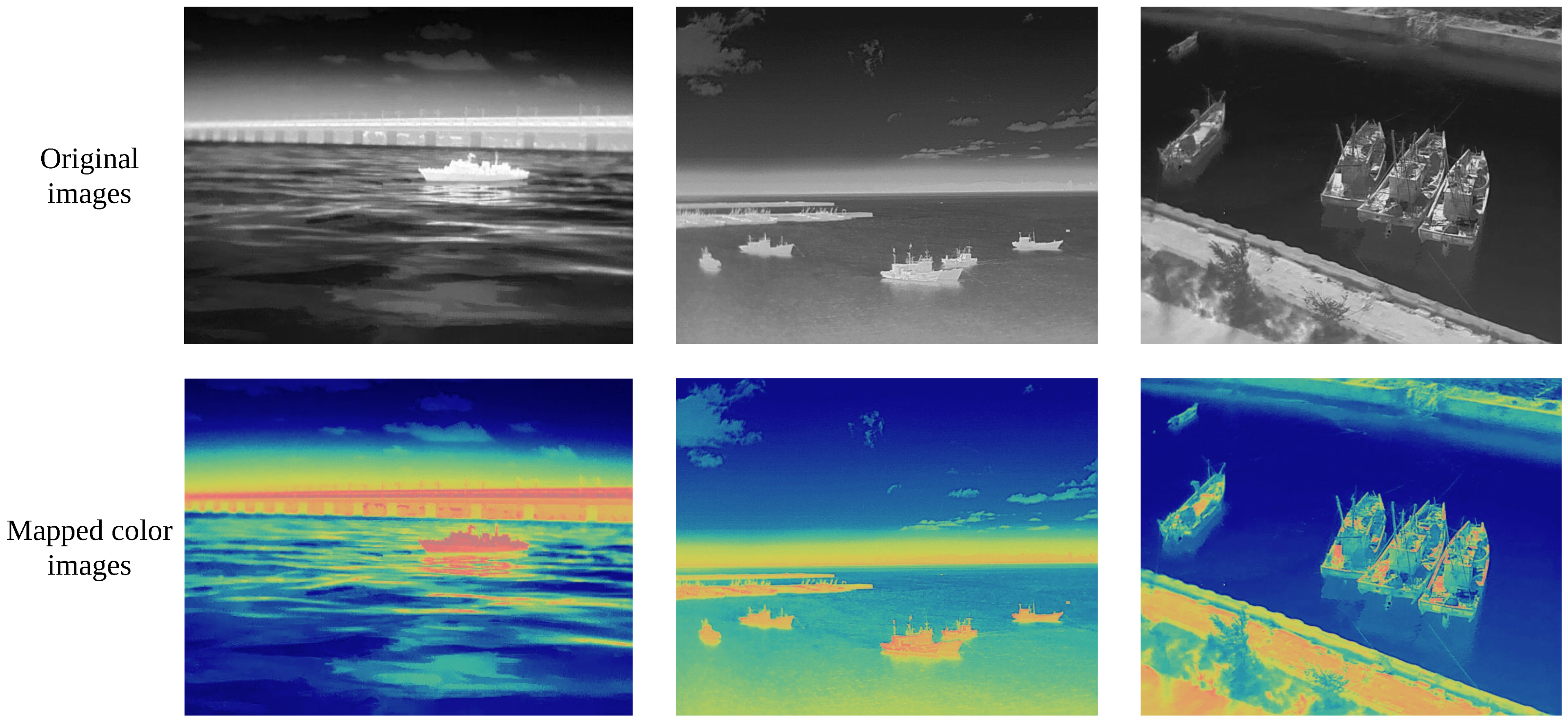
In nature, any object with a temperature above absolute zero (0 K) emits infrared radiation. Infrared images are formed by capturing the thermal radiation emitted by objects, resulting in different brightness levels corresponding to temperature differences. As shown in Figure 4, the three scenarios all demonstrate a clear difference in brightness levels between the ship targets and their backgrounds. Ships in infrared images typically have higher temperatures compared to their background, such as water surfaces, making them appear brighter in infrared images. This characteristic can be leveraged to assist in object detection.
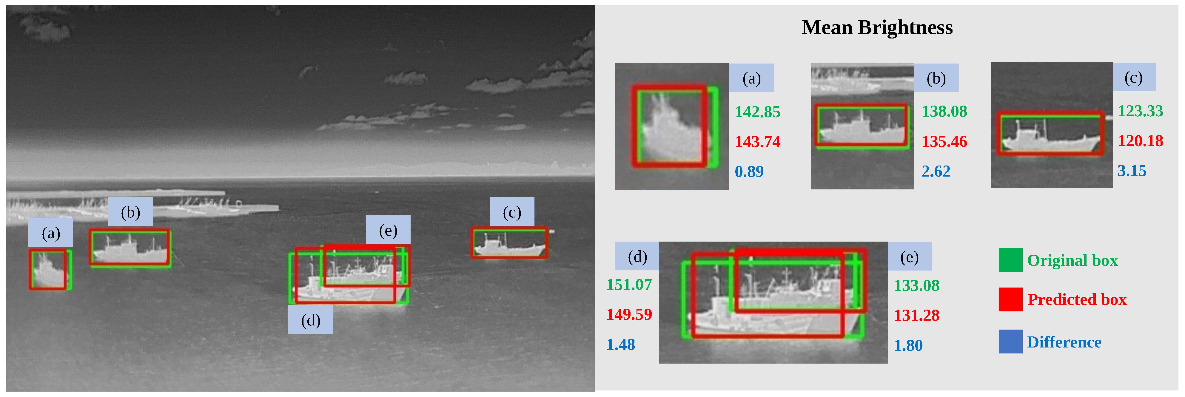
As shown in 
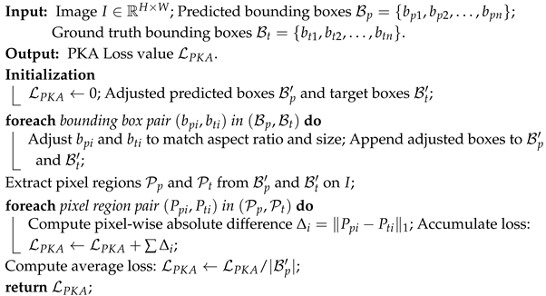
Figure 5, the mean brightness of each target bounding box in the infrared ship image is displayed. It can be observed that there is a noticeable difference in the mean brightness between the ground truth (GT) bounding box and the predicted bounding box. Specifically, for ship (c), the brightness difference between the two boxes reaches 3.15. This significant difference in mean brightness indicates that the predicted bounding box does not fully align with the target, suggesting that some portions of the ship’s main body are not accurately captured within the predicted box. This misalignment leads to the observed discrepancy in average brightness. To address this issue, Prior Knowledge Auxiliary (PKA) Loss was designed by incorporating the brightness differences between the GT and predicted bounding boxes of infrared ships as prior knowledge. The PKA Loss is combined with the CIoU from vanilla YOLOv8 to form a new regression loss, named CPA Loss. The values obtained by normalizing the pixel values of the grayscale image to a range of 0 to 1 represent brightness. There is a significant difference in brightness distribution between the target and the background. This difference in brightness distribution is represented by the mean brightness. To ensure an accurate calculation of the mean brightness with an equal number of pixels in both target boxes, the width and height of the boxes are adjusted to be identical. As shown in Figure 6, the green box represents the original bounding box, and the red box represents the predicted bounding box. By fixing the center points of the target boxes, the width and height are adjusted to the minimum values of the width and height of the two boxes, respectively. The pseudo-code of PKA Loss is shown in Algorithm 1.
Algorithm 1: Pseudo-code of PKA Loss
Jmse 13 00226 i001
The new regression loss, CPA Loss, is obtained by combining CIoU with the PKA Loss at different weight ratios:
L P K A = i = 1 | B p | j = 1 N i P p i ( j ) P t i ( j ) 1 | B p | ,
L C P A = ω L C I o U + ( 1 ω ) L P K A ,
where L P K A represents the PKA Loss value, P p i ( j ) is the brightness value of the predicted bounding box, P t i ( j ) is the brightness value of the original bounding box, P p i ( j ) P t i ( j ) 1 is the pixel-level difference, N i is the number of pixels in each bounding box, B p is the number of pixels in each bounding box, ω is the loss weight ratio, and L C I o U is the CIoU Loss value.

4. Experimental Results

4.1. Experimental Settings

The operating system used in this experiment is Ubuntu, with an Intel Core i9 10920x CPU and an Nvidia GeForce RTX 4090 GPU. The deep learning framework employed is PyTorch-GPU 2.1.1, with CUDA version 12.1. The programming language used is Python 3.8.
The number of training epochs is set to 300, with a batch size of 16. The warm-up batch size is set to 5. The optimizer used is SGD with a momentum of 0.937. The initial learning rate is 0.01, and the learning rate decay strategy employs the cosine annealing algorithm.
To enrich the background and increase the quantity of small objects, mosaic data augmentation is employed during the training process. This involves randomly cropping, scaling, and arranging four images and then concatenating them into a single image.

4.2. Datasets

The SFISD dataset [35] consists of 1070 infrared ship images, including single targets, multiple targets, dense targets, and overlapping targets. The dataset comprises 749 images for training and 321 images for testing. The InfiRray Ships dataset (www.iraytek.com (accessed on 15 June 2024)) contains a total of 8402 images of seven classes of infrared ships captured in various scenarios, with 6721 images for training and 1681 images for testing. As shown in Figure 7, the width and height of infrared ship images were normalized to analyze the scale distribution of ship targets. This normalization process involved dividing the width of the bounding box by the image width and the height of the bounding box by the image height, resulting in normalized width and height values ranging between 0 and 1. Statistical analysis of these normalized values revealed the presence of multi-scale ship targets in both datasets, with a significant proportion of small targets. The experiments in this paper were based on the two datasets mentioned above.

4.3. Evaluation Metrics

To assess the performance of the object detection model, standard evaluation metrics, such as mean value of average precision (mAP), parameters, and floating-point operations per second, are used in this study. AP (average precision) refers to the area under the precision–recall (P-R) curve, with recall as the horizontal axis and precision as the vertical axis. The calculation is expressed as Equation (13):
A P = 0 1 p ( r ) d r ,
where p represents precision, and r represents recall.
To provide a more detailed evaluation of the model’s performance across different object sizes, the metrics APS, APM, and APL are used. APS is the AP value for detecting small objects with pixel sizes less than 32 × 32, while APL is the AP value for detecting large objects with pixel sizes greater than 96 × 96. Additionally, mAP50 and mAP75 represent the average precision at IoU thresholds of 0.50 and 0.75, respectively. mAP50:95 refers to the mean average precision calculated over 10 mAP values, where the IoU threshold ranges from 0.50 to 0.95 with intervals of 0.05. The mAP is the mean of the AP values for each category, and the calculation is expressed as Equation (14):
m A P = Σ i = 1 C A P i c ,
where c represents the number of classes, and A P i represents the mean average precision for the i-th category.

4.4. Results and Analysis

4.4.1. Quantitative Results

To validate the infrared ship detection performance of the proposed PJ-YOLO, we compared it with nine state-of-the-art methods, including FCOS [36], CenterNet [37], TOOD [38], Sparse R-CNN [39], MFPRN [12], RT-DETR-r18 [21], YOLOv8 [13], YOLOv9 [20], and YOLOv10 [40]. RT-DETR-r18 refers to using ResNet18 as the backbone. The YOLO series networks are all compared using versions with a similar scale to the proposed PJ-YOLO. The proposed method was separately trained and tested on the SFISD dataset and the InfiRray Ships dataset. Our method outperforms the others based on the experimental results from both datasets.
(1)
Experiments on the SFISD dataset
The experimental comparison results on the SFISD dataset are shown in Table 1. Compared to the baseline method, the proposed PJ-YOLO demonstrates improvements of 1.6%, 5.0%, and 2.8% in mAP50, mAP75, and mAP50:95, respectively. Notably, PJ-YOLO achieves a remarkable 5.0% improvement in APS for small object detection and maintains superior performance across various target sizes.
(2)
Experiments on the InfiRray Ships dataset
The experimental comparison results on the InfiRray Ships dataset are shown in Table 2. Compared to the baseline method, the proposed PJ-YOLO demonstrates improvements of 1.0%, 2.1%, and 2.1% in mAP50, mAP75, and mAP50:95, respectively. The detailed category-wise comparison results are presented in Table 3. It can be seen that compared to the SOTA methods, the proposed PJ-YOLO shows significant improvements in metrics for each category of ship targets. Specifically, for individual categories, PJ-YOLO achieves the best results in all categories.

4.4.2. Qualitative Results

The visual comparison results on the SFISD dataset are shown in Figure 8. From left to right, the figures display the ground truth (GT) and the visualization results of YOLOv8, YOLOv9, YOLOv10, and PJ-YOLO, respectively. In Figure 8a, YOLOv9 mistakenly identifies the background on the left as a ship target, and YOLOv10 fails to detect the small target in the center. In Figure 8b, YOLOv9 fails to detect the ship target on the left, while YOLOv10 mistakenly identifies the shoreline as a ship target. In Figure 8c, both YOLOv8 and YOLOv9 mistakenly identify the background as ship targets, and YOLOv9 and YOLOv10 fail to detect the small target on the right. In Figure 8d,e, YOLOv8, YOLOv9, and YOLOv10 exhibit missed detections for small targets. The proposed PJ-YOLO effectively addresses the issues of missed detections and false positives prevalent in other methods, demonstrating superior performance in detecting infrared ship targets across various scales.
The visual comparison results on the InfiRray Ships dataset are shown in Figure 9. In Figure 9a, YOLOv8 and YOLOv10 fail to detect the target, and YOLOv9 misidentifies a canoe as a warship. In contrast, the proposed PJ-YOLO accurately detects the target. In Figure 9b, YOLOv9 and YOLOv10 misclassify the bulk carrier as another category. In Figure 9c, YOLOv8 and YOLOv10 fail to detect the ships that are close to the shore. Figure 9d depicts a relatively blurry scene. In Figure 9d, YOLOv8, YOLOv9, and YOLOv10 all exhibit false detections, incorrectly identifying shore objects and structures as ships, whereas the proposed PJ-YOLO accurately distinguishes between these objects and true ship targets. In Figure 9e, other methods exhibit numerous instances of missed detections, whereas the proposed PJ-YOLO accurately identifies all the targets. Through comparisons in diverse scenarios, the superior performance and robustness of our proposed method are clearly illustrated.
Grad-CAM [41] is a technique that highlights the regions in the input image that are the most important for the model’s prediction. Visualization experiments using Grad-CAM were conducted on the baseline method and the proposed PJ-YOLO. By utilizing the gradient information from the feature map, the corresponding weights were generated to obtain heatmaps. The comparison of image heatmaps across different stages is shown in Figure 10. It can be observed that the class activation mapping of PJ-YOLO focuses more on the target area, while the baseline method exhibits a scattered attention pattern, focusing not only on the target but also on irrelevant regions such as the shore and non-ship areas on the water surface. Guided by prior knowledge of infrared ships, the proposed JFE module enhances the network’s feature extraction capability, enabling it to concentrate more on the target area of infrared ships.

4.5. Ablation Study

To better explore the detection performance of the PJ-YOLO proposed in this paper and verify the efficacy of each module, we conducted ablation experiments on the SFISD dataset. Ablation experiment comparisons are shown in Table 4. The JFE module improves the model’s mAP50 by 0.7%, mAP75 by 1.2%, and the mAP50:95 by 0.6%. Introducing the R-DA attention module further increases the mAP50 by 0.4%, mAP75 by 0.6%, and the mAP50:95 by 0.9%. Additionally, the introduction of PKA Loss brings about further improvements in performance. However, with the model improvements, the parameters and computational complexity of the model also increase.
The visualization results of the ablation study are shown in Figure 11. By comparing the performance of the baseline model with the incremental addition of the JFE module, R-DA attention module, and PKA Loss, the figure illustrates the performance improvements contributed by each module to the overall model. It can be observed that the issues of missed detections and false detections have been improved and resolved.
To evaluate the effectiveness of the CPA Loss, we specifically designed a series of ablation experiments on the SFISD dataset, where comparisons were performed between CPA Loss and other loss functions including GIoU [42], DIoU [43], SIoU [44], EIoU [45], and CIoU [43]. The experimental results, shown in Table 5, clearly demonstrate that CPA Loss outperforms other loss functions in the task of infrared ship detection and has a positive impact on improving the overall performance of the model.
To investigate the impact of different weight ratios between CIoU Loss and PKA Loss in the regression loss component, five sets of ablation experiments were designed on the SFISD dataset. The comparison results are shown in Table 6.

4.6. Computational Complexity

To evaluate the computational complexity of the proposed PJ-YOLO, a comparative experiment was conducted with the batch size set to 1 to simulate real-world scenarios. Figure 12 demonstrates the computational complexity comparisons between PJ-YOLO and other competing methods. Initially, the computational complexity of different methods is evaluated based on latency and floating-point operations (FLOPs), and the performance of these methods is evaluated using the SFISD dataset.
The real-time performance comparison results are presented in Table 7. The proposed PJ-YOLO achieves 87.7 FPS. As illustrated in Table 7, while its FPS is marginally lower and its latency is somewhat increased compared to some baseline models, it still fulfills the requirements for real-time processing. The proposed PJ-YOLO showcases significant practical value for scenarios demanding immediate responsiveness, effectively balancing performance with speed, and holds potential for real-world applications in infrared ship detection tasks.

4.7. Performance Evaluation in Real-World Scenes

To evaluate the generalization capability of the proposed PJ-YOLO, the model trained on the SFISD dataset was utilized for detecting ships on real-world infrared images collected from the Internet. The visualization of prediction results is presented in Figure 13. In Figure 13a, both YOLOv8 and YOLOv10 fail to detect the ship target, and YOLOv9 mistakenly identifies the watermark as a ship target. In Figure 13b, YOLOv8, YOLOv9, and YOLOv10 all mistakenly identify the island on the left side of the image as a ship target. In Figure 13c, YOLOv8, YOLOv9, and YOLOv10 all exhibit numerous false detections. In comparison, the proposed PJ-YOLO successfully detects ship targets without any false alarms, demonstrating better detection capability and highlighting its enhanced generalization ability.

5. Conclusions

In this paper, we proposed a PJ-YOLO for infrared ship detection, which is dedicated to improving detection performance. In the feature extraction stage, a joint feature extraction module was designed to enhance the extraction of effective features from multiple dimensions. To enhance the model’s focus on targets of different scales, we introduced a residual deformable attention mechanism at the high level of the backbone network, improving the capture of target features. Additionally, we designed a prior auxiliary loss using prior knowledge of infrared ship brightness distribution to more accurately locate targets, enhancing the model’s robustness and improving target localization accuracy. Extensive experiments on the SFISD dataset and the InfiRray Ships dataset validate that PJ-YOLO significantly improves the detection accuracy of infrared ships.
Future research will focus on lightweighting the network structure to enhance FPS while maintaining high detection accuracy, thereby improving operational efficiency and reducing computational resource consumption. To achieve this, we will explore techniques such as network pruning, model lightweighting, operator optimization, and knowledge distillation. Additionally, to enhance the model’s generalization capability, we will also focus on collecting a more diverse set of infrared ship images, aiming to ensure that it maintains stable and efficient performance across various real-world conditions.

Author Contributions

Conceptualization, Y.L. and C.L.; methodology, Y.L.; software, Y.L.; validation, Y.L. and C.L.; formal analysis, Y.L.; investigation, C.L.; resources, C.L.; data curation, Y.L.; writing—original draft preparation, Y.L.; writing—review and editing, C.L. and G.F.; visualization, Y.L.; supervision, C.L. and G.F.; project administration, C.L. and G.F.; funding acquisition, C.L. and G.F. All authors have read and agreed to the published version of the manuscript.

Funding

This research was funded by the National Natural Science Foundation of China, grant number 62176150.

Institutional Review Board Statement

Not applicable.

Informed Consent Statement

Not applicable.

Data Availability Statement

Data will be available as requested.

Conflicts of Interest

The authors declare no conflicts of interest.

References

  1. Ye, J.; Li, C.; Wen, W.; Zhou, R.; Reppa, V. Deep Learning in Maritime Autonomous Surface Ships: Current Development and Challenges. J. Mar. Sci. Appl. 2023, 22, 584–601. [Google Scholar] [CrossRef]
  2. Liu, Y.; Su, H.; Zeng, C.; Li, X. A Robust Thermal Infrared Vehicle and Pedestrian Detection Method in Complex Scenes. Sensors 2021, 21, 1240. [Google Scholar] [CrossRef] [PubMed]
  3. Li, J.; Gong, W.; Li, W.; Liu, X. Robust Pedestrian Detection in Thermal Infrared Imagery Using the Wavelet Transform. Infrared Phys. Technol. 2010, 53, 267–273. [Google Scholar] [CrossRef]
  4. He, H.; Hu, Z.; Wang, B.; Luo, D.; Lee, W.J.; Li, J. A Contactless Zero-Value Insulators Detection Method Based on Infrared Images Matching. IEEE Access 2020, 8, 133882–133889. [Google Scholar] [CrossRef]
  5. Liu, J.; He, Z.; Chen, Z.; Shao, L. Tiny and Dim Infrared Target Detection Based on Weighted Local Contrast. IEEE Geosci. Remote Sens. Lett. 2018, 15, 1780–1784. [Google Scholar] [CrossRef]
  6. Zhang, Y.; Li, C.; Shang, S.; Chen, X. SwinSeg: Swin Transformer and MLP Hybrid Network for Ship Segmentation in Maritime Surveillance System. Ocean Eng. 2023, 281, 114885. [Google Scholar] [CrossRef]
  7. Zhong, X.; Wang, M.; Liu, W.; Yuan, J.; Huang, W. SCPNet: Self-constrained Parallelism Network for Keypoint-Based Lightweight Object Detection. J. Vis. Commun. Image Represent. 2023, 90, 103719. [Google Scholar] [CrossRef]
  8. Mo, Y.; Li, C. Contrastive Adaptive Frequency Decomposition Network Guided by Haze Discrimination for Real-World Image Dehazing. Displays 2024, 82, 102665. [Google Scholar] [CrossRef]
  9. Wen, G.; Cao, P.; Wang, H.; Chen, H.; Liu, X.; Xu, J.; Zaiane, O. MS-SSD: Multi-Scale Single Shot Detector for Ship Detection in Remote Sensing Images. Appl. Intell. 2023, 53, 1586–1604. [Google Scholar] [CrossRef]
  10. Zhan, W.; Zhang, C.; Guo, S.; Guo, J.; Shi, M. EGISD-YOLO: Edge Guidance Network for Infrared Ship Target Detection. IEEE J. Sel. Top. Appl. Earth Obs. Remote Sens. 2024, 17, 10097–10107. [Google Scholar] [CrossRef]
  11. Li, L.; Jiang, L.; Zhang, J.; Wang, S.; Chen, F. A Complete YOLO-based Ship Detection Method for Thermal Infrared Remote Sensing Images under Complex Backgrounds. Remote Sens. 2022, 14, 1534. [Google Scholar] [CrossRef]
  12. Yuan, J.; Cai, Z.; Wang, S.; Kong, X. A Multitype Feature Perception and Refined Network for Spaceborne Infrared Ship Detection. IEEE Trans. Geosci. Remote Sens. 2024, 62, 1–11. [Google Scholar] [CrossRef]
  13. Jocher, G.; Qiu, J.; Chaurasia, A. Ultralytics YOLO. 2023. Available online: https://github.com/ultralytics/ultralytics (accessed on 10 June 2024).
  14. Girshick, R. Fast R-CNN. In Proceedings of the 2015 IEEE International Conference on Computer Vision (ICCV), Santiago, Chile, 7–13 December 2015; pp. 1440–1448. [Google Scholar] [CrossRef]
  15. Ren, S.; He, K.; Girshick, R.; Sun, J. Faster R-CNN: Towards Real-Time Object Detection with Region Proposal Networks. IEEE Trans. Pattern Anal. Mach. Intell. 2017, 39, 1137–1149. [Google Scholar] [CrossRef]
  16. Cai, Z.; Vasconcelos, N. Cascade R-CNN: High Quality Object Detection and Instance Segmentation. IEEE Trans. Pattern Anal. Mach. Intell. 2021, 43, 1483–1498. [Google Scholar] [CrossRef] [PubMed]
  17. Liu, W.; Anguelov, D.; Erhan, D.; Szegedy, C.; Reed, S.; Fu, C.Y.; Berg, A.C. SSD: Single Shot MultiBox Detector. In Proceedings of the Computer Vision—ECCV, Amsterdam, The Netherlands, 11–14 October 2016; pp. 21–37. [Google Scholar] [CrossRef]
  18. Lin, T.Y.; Goyal, P.; Girshick, R.; He, K.; Dollár, P. Focal Loss for Dense Object Detection. In Proceedings of the 2017 IEEE International Conference on Computer Vision (ICCV), Venice, Italy, 22–29 October 2017; pp. 2999–3007. [Google Scholar] [CrossRef]
  19. Redmon, J.; Divvala, S.; Girshick, R.; Farhadi, A. You Only Look Once: Unified, Real-Time Object Detection. In Proceedings of the 2016 IEEE Conference on Computer Vision and Pattern Recognition (CVPR), Las Vegas, NV, USA, 27–30 June 2016; pp. 779–788. [Google Scholar] [CrossRef]
  20. Wang, C.Y.; Yeh, I.H.; Mark Liao, H.Y. YOLOv9: Learning What You Want to Learn Using Programmable Gradient Information. In Proceedings of the Computer Vision—ECCV 2024, Milan, Italy, 29 September–4 October 2024; pp. 1–21. [Google Scholar] [CrossRef]
  21. Zhao, Y.; Lv, W.; Xu, S.; Wei, J.; Wang, G.; Dang, Q.; Liu, Y.; Chen, J. DETRs Beat YOLOs on Real-Time Object Detection. In Proceedings of the IEEE/CVF Conference on Computer Vision and Pattern Recognition, Seattle, WA, USA, 16–22 June 2024; pp. 16965–16974. [Google Scholar]
  22. Zhu, H.; Liu, S.; Deng, L.; Li, Y.; Xiao, F. Infrared Small Target Detection via Low-Rank Tensor Completion with Top-Hat Regularization. IEEE Trans. Geosci. Remote Sens. 2020, 58, 1004–1016. [Google Scholar] [CrossRef]
  23. Liu, T.; Yin, Q.; Yang, J.; Wang, Y.; An, W. Combining Deep Denoiser and Low-Rank Priors for Infrared Small Target Detection. Pattern Recognit. 2023, 135, 109184. [Google Scholar] [CrossRef]
  24. Gao, Z.; Yin, J.; Luo, J.; Li, W.; Peng, Z. Multidirectional Graph Learning-Based Infrared Cirrus Detection with Local Texture Features. IEEE Trans. Geosci. Remote Sens. 2023, 61, 5004020. [Google Scholar] [CrossRef]
  25. Zhang, C.; He, Y.; Tang, Q.; Chen, Z.; Mu, T. Infrared Small Target Detection via Interpatch Correlation Enhancement and Joint Local Visual Saliency Prior. IEEE Trans. Geosci. Remote Sens. 2022, 60, 5001314. [Google Scholar] [CrossRef]
  26. Xu, X.; Zhan, W.; Zhu, D.; Jiang, Y.; Chen, Y.; Guo, J. Contour Information-Guided Multi-Scale Feature Detection Method for Visible-Infrared Pedestrian Detection. Entropy 2023, 25, 1022. [Google Scholar] [CrossRef] [PubMed]
  27. Du, S.; Zhang, P.; Zhang, B.; Xu, H. Weak and Occluded Vehicle Detection in Complex Infrared Environment Based on Improved YOLOv4. IEEE Access 2021, 9, 25671–25680. [Google Scholar] [CrossRef]
  28. Bao, C.; Cao, J.; Hao, Q.; Cheng, Y.; Ning, Y.; Zhao, T. Dual-YOLO Architecture from Infrared and Visible Images for Object Detection. Sensors 2023, 23, 2934. [Google Scholar] [CrossRef] [PubMed]
  29. Jiang, X.; Cai, W.; Yang, Z.; Xu, P.; Jiang, B. IARet: A Lightweight Multiscale Infrared Aerocraft Recognition Algorithm. Arab. J. Sci. Eng. 2022, 47, 2289–2303. [Google Scholar] [CrossRef]
  30. Kera, S.B.; Tadepalli, A.; Ranjani, J.J. A Paced Multi-Stage Block-Wise Approach for Object Detection in Thermal Images. Vis. Comput. 2023, 39, 2347–2363. [Google Scholar] [CrossRef]
  31. Zhou, W.; Ben, T. IRMultiFuseNet: Ghost Hunter for Infrared Ship Detection. Displays 2024, 81, 102606. [Google Scholar] [CrossRef]
  32. Liu, J.J.; Hou, Q.; Cheng, M.M.; Wang, C.; Feng, J. Improving Convolutional Networks with Self-Calibrated Convolutions. In Proceedings of the 2020 IEEE/CVF Conference on Computer Vision and Pattern Recognition (CVPR), Seattle, WA, USA, 13–19 June 2020; pp. 10093–10102. [Google Scholar] [CrossRef]
  33. Ding, X.; Zhang, X.; Ma, N.; Han, J.; Ding, G.; Sun, J. RepVGG: Making VGG-style ConvNets Great Again. In Proceedings of the IEEE/CVF Conference on Computer Vision and Pattern Recognition, Nashville, TN, USA, 20–25 June 2021; pp. 13733–13742. [Google Scholar]
  34. Xia, Z.; Pan, X.; Song, S.; Li, L.E.; Huang, G. Vision Transformer with Deformable Attention. In Proceedings of the IEEE/CVF Conference on Computer Vision and Pattern Recognition, New Orleans, LA, USA, 18–24 June 2022; pp. 4794–4803. [Google Scholar]
  35. Wu, P.; Su, S.; Tong, X.; Guo, R.; Sun, B.; Zuo, Z.; Zhang, J. SARFB: Strengthened Asymmetric Receptive Field Block for Accurate Infrared Ship Detection. IEEE Sens. J. 2023, 23, 5028–5044. [Google Scholar] [CrossRef]
  36. Tian, Z.; Shen, C.; Chen, H.; He, T. FCOS: Fully Convolutional One-Stage Object Detection. In Proceedings of the 2019 IEEE/CVF International Conference on Computer Vision (ICCV), Seoul, Republic of Korea, 27 October–2 November 2019; pp. 9626–9635. [Google Scholar] [CrossRef]
  37. Duan, K.; Bai, S.; Xie, L.; Qi, H.; Huang, Q.; Tian, Q. CenterNet: Keypoint Triplets for Object Detection. In Proceedings of the 2019 IEEE/CVF International Conference on Computer Vision (ICCV), Seoul, Republic of Korea, 27 October–2 November 2019; pp. 6568–6577. [Google Scholar] [CrossRef]
  38. Feng, C.; Zhong, Y.; Gao, Y.; Scott, M.R.; Huang, W. TOOD: Task-aligned One-Stage Object Detection. In Proceedings of the 2021 IEEE/CVF International Conference on Computer Vision (ICCV), Montreal, QC, Canada, 10–17 October 2021; pp. 3490–3499. [Google Scholar] [CrossRef]
  39. Sun, P.; Zhang, R.; Jiang, Y.; Kong, T.; Xu, C.; Zhan, W.; Tomizuka, M.; Yuan, Z.; Luo, P. Sparse R-CNN: An End-to-End Framework for Object Detection. IEEE Trans. Pattern Anal. Mach. Intell. 2023, 45, 15650–15664. [Google Scholar] [CrossRef]
  40. Wang, A.; Chen, H.; Liu, L.; Chen, K.; Lin, Z.; Han, J.; Ding, G. YOLOv10: Real-Time End-to-End Object Detection. arXiv 2024, arXiv:2405.14458. [Google Scholar] [CrossRef]
  41. Selvaraju, R.R.; Cogswell, M.; Das, A.; Vedantam, R.; Parikh, D.; Batra, D. Grad-CAM: Visual Explanations from Deep Networks via Gradient-Based Localization. In Proceedings of the 2017 IEEE International Conference on Computer Vision (ICCV), Venice, Italy, 22–29 October 2017; pp. 618–626. [Google Scholar] [CrossRef]
  42. Rezatofighi, H.; Tsoi, N.; Gwak, J.; Sadeghian, A.; Reid, I.; Savarese, S. Generalized Intersection over Union: A Metric and a Loss for Bounding Box Regressio. arXiv 2019, arXiv:1902.09630. [Google Scholar] [CrossRef]
  43. Zheng, Z.; Wang, P.; Liu, W.; Li, J.; Ye, R.; Ren, D. Distance-IoU Loss: Faster and Better Learning for Bounding Box Regression. arXiv 2019, arXiv:1911.08287. [Google Scholar] [CrossRef]
  44. Gevorgyan, Z. SIoU Loss: More Powerful Learning for Bounding Box Regression. arXiv 2022, arXiv:2205.12740. [Google Scholar] [CrossRef]
  45. Zhang, Y.F.; Ren, W.; Zhang, Z.; Jia, Z.; Wang, L.; Tan, T. Focal and Efficient IOU Loss for Accurate Bounding Box Regression. arXiv 2022, arXiv:2101.08158. [Google Scholar] [CrossRef]
Figure 1. Overall architecture of PJ-YOLO.
Jmse 13 00226 g001
Figure 2. Structure of the JFE module.
Jmse 13 00226 g002
Figure 3. Structure of the R-DA module.
Jmse 13 00226 g003
Figure 4. Brightness distribution of the infrared ship image.
Jmse 13 00226 g004
Figure 5. Mean brightness of the bounding box. In the right image, (ae) are extracted from the left image, each containing the ground truth (GT) bounding box and the predicted bounding box. Green numbers represent the mean brightness values of pixels within the ground truth (GT) bounding boxes, while red numbers represent the mean brightness values of pixels within the predicted bounding boxes. Blue numbers indicate the difference in mean brightness between the GT and predicted bounding boxes. A larger difference value indicates a greater discrepancy in brightness distribution.
Jmse 13 00226 g005
Figure 6. Bounding box adjustment process in PKA Loss: green box (GT) and red box (predicted).
Jmse 13 00226 g006
Figure 7. The size distribution of targets in the datasets: (a) the SFISD dataset and (b) the InfiRray Ships dataset. The darker the dot color, the larger the quantity of targets with normalized width and height.
Jmse 13 00226 g007
Figure 8. Visual comparison of results for the SFISD dataset. False negative samples are highlighted with blue circles, and false positive samples are indicated with purple circles.
Jmse 13 00226 g008
Figure 9. Visual comparison of results for the InfiRray Ships dataset. False negative samples are highlighted with blue circles, and false positive samples are indicated with purple circles.
Jmse 13 00226 g009
Figure 10. Grad-CAM visualization results for different stages of the baseline network and PJ-YOLO across diverse scenarios in the InfiRray Ships dataset: (a) single-target scenario and (b) multi-target scenario.
Jmse 13 00226 g010
Figure 11. Visualization results of the ablation study from multiple scenarios.
Jmse 13 00226 g011
Figure 12. Comparison of latency, FLOPs, and mAP50:95 (on the SFISD dataset) between PJ-YOLO and other competing methods. The number of FLOPs is represented by the radius of the circle.
Jmse 13 00226 g012
Figure 13. Visualization comparison of prediction results on real-world images.
Jmse 13 00226 g013
Table 1. Performance of different methods on the SFISD dataset.
MethodYearmAP50mAP75mAP50:95APSAPMAPLParams (M)FLOPs (G)
FCOS [36]201972.651.548.36.844.874.531.851.5
CenterNet [37]201988.152.551.312.546.072.432.7109.7
TOOD [38]202179.350.647.57.344.173.832.074.4
Sparse R-CNN [39]202383.247.447.514.044.874.0106.043.0
MFPRN [12]202384.056.552.610.250.776.764.6178.0
RT-DETR-r18 [21]202492.867.961.319.655.377.920.060.0
YOLOv8 [13]202392.069.263.017.657.280.311.228.6
YOLOv9 [20]202491.968.862.313.157.780.27.126.4
YOLOv10 [40]202492.168.761.619.655.778.97.221.6
PJ-YOLO 93.674.265.822.658.380.515.235.3
Note: Bold value indicates the best results on the evaluation metrics.
Table 2. Performance of different methods on the InfiRray Ships dataset.
MethodYearmAP50mAP75mAP50:95APSAPMAPLParams (M)FLOPs (G)
FCOS [36]201984.258.154.532.456.868.631.851.5
CenterNet [37]201987.359.155.631.656.968.132.7109.7
TOOD [38]202185.360.256.734.758.170.732.074.4
Sparse R-CNN [39]202390.761.259.034.740.272.2106.043.0
MFPRN [12]202389.664.760.439.161.872.464.6178.0
RT-DETR-r18 [21]202493.269.164.344.465.476.920.060.0
YOLOv8 [13]202392.669.865.343.863.076.711.228.6
YOLOv9 [20]202491.566.863.141.663.075.67.126.4
YOLOv10 [40]202492.569.664.643.563.374.87.221.6
PJ-YOLO 93.671.967.445.664.878.715.235.3
Note: Bold value indicates the best results on the evaluation metrics.
Table 3. Performance of different methods on specific categories on the InfiRray Ships dataset.
MethodAP50:95
All Liner Bulk Warship Sailboat Canoe Container Fishing
FCOS [36]54.547.272.674.144.137.374.132.2
CenterNet [37]55.647.172.775.646.040.374.732.6
TOOD [38]56.746.575.777.246.338.376.336.8
Sparse R-CNN [39]59.047.976.678.448.041.278.442.5
MFPRN [12]60.449.476.479.850.342.779.444.7
RT-DETR-r18 [21]64.355.579.881.255.749.880.248.0
YOLOv8 [13]65.359.082.583.757.851.575.646.8
YOLOv9 [20]63.156.179.180.956.749.676.343.4
YOLOv10 [40]64.659.279.282.356.850.777.846.4
PJ-YOLO67.461.083.585.459.154.080.348.8
Note: The results in bold font and underlined indicate the best and suboptimal results on the evaluation metric, respectively.
Table 4. Ablation experiment of each module.
MethodJFER-DAPKA LossmAP50mAP75mAP50:95Params (M)FLOPs (G)
Baseline---92.069.263.011.228.6
1--92.770.463.615.035.2
2-93.171.064.515.235.3
3-93.472.464.615.035.2
493.674.265.815.235.3
Table 5. Ablation study on the comparison of different loss functions.
LossmAP50mAP75mAP50:95
GIoU [42]93.170.363.7
DIoU [43]93.071.263.9
SIoU [44]92.971.164.2
EIoU [45]92.971.063.3
CIoU [43]93.171.064.5
CPA93.674.265.8
Table 6. Ablation experiment of weight ratios.
ω CIoU ω PKA mAP50mAP75mAP50:95
1093.171.064.5
0.80.293.272.665.1
0.60.493.674.265.8
0.40.693.972.364.4
0.20.893.471.865.0
Table 7. Comparison of FPS and latency for different methods.
MethodRT-DETR-r18YOLOv8YOLOv9YOLOv10PJ-YOLO
FPS49.0158.767.1133.387.7
Latency (ms)20.46.314.97.511.4
Disclaimer/Publisher’s Note: The statements, opinions and data contained in all publications are solely those of the individual author(s) and contributor(s) and not of MDPI and/or the editor(s). MDPI and/or the editor(s) disclaim responsibility for any injury to people or property resulting from any ideas, methods, instructions or products referred to in the content.

