1. Introduction
Traditional methods for predicting coastal dynamics often rely on numerical models, which can be computationally expensive and may not fully capture the complex non-linear interactions in these systems. Machine learning offers a promising alternative with the potential to improve prediction accuracy and efficiency.
The increasing accessibility of comprehensive geospatial marine data, as provided by services like Copernicus Marine Service (CMEMS) [
1], has opened new paths for understanding and predicting coastal dynamics. Integrating these modelled data with in-situ observations represents the key to refining prediction accuracies and appropriating localized phenomena.
Several studies have demonstrated the potential of Artificial Intelligence (AI) and Machine Learning (ML) techniques in bridging this gap and enhancing coastal dynamics prediction. Mihailov et al. [
2,
3] used machine learning to improve the accuracy of sea level predictions in the Black Sea, demonstrating the potential of AI/ML in this region. Similarly, Campos et al. [
4] used neural networks to refine wave ensemble forecasts by post-processing outputs from the National Centers for Environmental Prediction (NCEP)’s Global Wave Ensemble Forecast System (GWES) addressing limitations of numerical weather prediction models. This approach addresses the inherent limitations of numerical weather prediction models by refining their predictions through statistical learning from observational data. Furthermore, Lee et al. (2007) [
5] combined harmonic analysis with artificial neural networks (ANN) to achieve more accurate tidal predictions, showcasing the potential of integrating machine learning with traditional methods for improved prediction in coastal environments. The increasing role of machine learning in addressing the limitations of numerical weather prediction is further emphasized by Schultz et al. [
6], explored the potential of deep learning to improve and potentially replace traditional numerical weather models, leading to more efficient and accurate weather forecasting systems.
One of the key challenges in integrating in-situ and modelled data is addressing discrepancies and uncertainties arising from different spatial and temporal resolutions and inherent biases in each data source. Recent advancements in AI/ML offer robust tools for data fusion and bias correction. Jung et al. [
7] used a deep learning approach to fuse satellite-derived sea surface temperature with in-situ measurements, demonstrating improved accuracy in coastal temperature predictions. Likewise, Makarynskyy [
8] utilized a machine learning-based data assimilation technique to integrate modelled wave data with buoy observations, enhancing wave predictions in coastal regions. These studies employ various techniques to address discrepancies and uncertainties, including data normalization, bias correction, and spatio-temporal matching. For instance, deep learning models are used to fuse satellite-derived data with in-situ measurements, while machine learning-based data assimilation techniques integrate modelled data with buoy observations. These approaches aim to create a unified dataset that accurately represents the coastal dynamics while accounting for each data source’s inherent biases and limitations.
Grad-CAM, or Gradient-weighted Class Activation Mapping [
9], is a powerful visualization technique that provides insights into the decision-making processes of deep learning models by generating heatmaps that indicate the regions of input data that most influence the model’s predictions. This capability is particularly valuable in fields such as meteorology and oceanography, where understanding the underlying factors driving model outputs is crucial for effective decision-making and management. The application of Grad-CAM in meteorological contexts has been explored in various studies, demonstrating its utility in interpreting model predictions. For instance, Choi et al. utilized Grad-CAM to enhance the interpretability of time-series predictions in meteorological models, showcasing how gradient-based methods can elucidate the relationships between input variables and model outputs [
10]. This aligns with the reviewer’s suggestion to incorporate a discussion of Grad-CAM in the context of our work, as it can provide a deeper understanding of the atmospheric influences on coastal dynamics along the Romanian Black Sea coast. Moreover, integrating Grad-CAM with other XAI techniques can further enhance model interpretability. For example, Diaz-Gomez et al. employed Grad-CAM in conjunction with occlusion analysis to assess the contributions of various input features to model predictions in medical imaging [
11]. This dual approach not only highlights the most influential regions in the input data but also allows for a more comprehensive understanding of the model’s decision-making process. Such methodologies can be adapted to our research, where understanding the impact of atmospheric conditions on marine dynamics is critical.
Machine learning models are increasingly used in coastal research to predict complex processes like sediment transport [
12,
13,
14], shoreline changes [
15,
16], and coastal flooding [
17,
18]. These AI/ML algorithms excel at identifying intricate patterns within large datasets, enabling more precise and rapid predictions. A study by [
19] further demonstrated the potential of machine learning for complex time-series forecasting in the Black Sea by predicting water temperature based on wind speed and air temperature.
Researchers increasingly focus on Explainable AI (XAI) to enhance confidence and transparency in AI-driven coastal management predictions. This field aims to explain the complexities of AI/ML models, providing insights into how these models arrive at their predictions. By close-fitting the causal factors and decision-making processes, XAI promotes a deeper understanding of the models’ behaviour and outputs. This is particularly important in hydroclimatic applications where the reliability and transparency of predictive models are influential [
20]. For instance, combining powerful AI models like XGBoost [
21], CatBoost [
22], and Random Forest [
23] with explanatory methods such as SHAP [
24] and LIME [
25] can significantly enhance the interpretability of AI-generated predictions. A practical example of XAI’s value is demonstrated in [
26], where researchers successfully interpreted a convolutional neural network (CNN) model used for flood prediction [
26,
27]. Their analysis revealed the dominant role of land use and soil attributes in driving flood events.
In the context of the Black Sea, integrating in-situ observations with modelled data from the CMEMS holds significant potential for improving coastal dynamics prediction along the Western coastline. The proposed research uses AI/ML techniques to address this region’s challenges and opportunities. By developing ML-based correlation systems and employing advanced regression and time series analysis, the research seeks to refine predictions of shallow water dynamics, particularly by considering atmospheric influences. The focus on wave-wind correlations and the investigation of extreme events further contribute to the novelty and relevance of this research. For example, refs. [
28,
29] used ANN’s to merge wave forecasts with field observations in a study focused on wave-wind correlations.
This research aims to achieve several key outcomes. Firstly, it seeks to enhance our comprehension of the intricate interplay between atmospheric conditions and marine processes. Secondly, it attempts to improve the precision of coastal dynamics predictions. Lastly, it aims to demonstrate the effectiveness of AI/ML in addressing gaps between observational data and model-generated data. These findings are expected to be instrumental in informing coastal zone management strategies and strengthening maritime safety along Romania’s Black Sea coastline.
Our study builds upon these advancements by utilizing Temporal Fusion Transformers (TFTs), a state-of-the-art deep learning architecture specifically designed for time series forecasting. TFTs have shown superior performance in various domains due to their ability to handle complex temporal dependencies and incorporate both static and time-varying features.
Our study integrates in-situ observations from coastal stations with modelled data provided by the CMEMS [
1,
30] to train and evaluate our TFT models. This approach allows us to represent local variability and regional patterns, which is significant for accurate coastal dynamics prediction. The following sections detail the data consolidation process, model training, performance evaluation, and key findings of our study.
2. Materials and Methods
The analysis utilizes a dataset of meteorological information collected by the Maritime Hydrographic Directorate (MHD) since 2015 [
31]. Specifically, the study relies on data gathered from seven automated weather stations at lighthouses along the Western coastline. These stations are part of the Romanian Navy’s Marine Meteorological Surveillance Network, which monitors regional weather conditions. The stations continuously gather meteorological parameters at specific ground-level heights, including wind speed and direction (
Figure 1).
The CMEMS wave reanalysis dataset for the Black Sea [
30] provides a comprehensive record of wave conditions with a spatial resolution of approximately 2.5 km and hourly temporal resolution. The model incorporates wave breaking and assimilates Jason’s satellite wave and wind data, utilizing European Centre for Medium-Range Weather Forecasts (ECMWF) Reanalysis v5 (ERA5) data for atmospheric forcing. In addition to the hourly wave data, the product includes a monthly climatology dataset and an air-sea flux dataset [
30].
Integrating in-situ observations with modelled data from the CMEMS offers an encouraging direction for enhancing the accuracy and comprehensiveness of coastal dynamics predictions. In-situ data from coastal stations provides valuable localized information on parameters such as wind speed, wave height, or current direction. However, these observations may be limited in spatial coverage and temporal resolution. Modelled data offers widespread spatial coverage and high temporal resolution, capturing regional patterns and dynamics. By combining these two data sources, we can link observational gaps and create a more complete and accurate representation of coastal dynamics. This integration allows for a deeper understanding of the interaction between local and regional factors influencing coastal or shallow water processes, leading to improved predictions.
The workflow illustrated in
Figure 2 integrates both in-situ data from coastal stations [
31] and modelled data from the CMEMS [
30]. The initial stage involves data preprocessing, where raw in-situ data, including wind and wave parameters, undergoes cleaning, formatting, and feature systematization. This step ensures data quality and consistency. Concurrently, relevant model outputs, such as wave forecasts, are acquired from the CMEMS. Next, data integration and consolidation occur. In-situ observations are spatially and temporally matched with CMEMS, followed by data fusion techniques to create a unified dataset. This consolidated dataset forms the foundation for subsequent model development.
Model selection ensues, with the image indicating the utilization of TFTs implemented in the PyTorch 2.4.0 framework [
34] integrated with pytorch-lightning [
35] version 2.4.0 and PyTorchorch forecasting version 1.1.1 [
36]. This choice aligns with the sophisticated machine learning approach employed in the research, as evidenced by the model result files showcasing TFTs’ ability to capture complex coastal dynamics.
The workflow then proceeds to model training, where the consolidated dataset is split into training, validation, and test sets. TFT models are trained using the training data, and hyperparameters are tuned via the validation set.
Following training, explainable AI techniques are employed to evaluate input parameter importance and gain insights into the model’s decision-making process. This step aligns with the emphasis on interpretability observed in the model result files, where variable importance plots highlight key factors influencing predictions.
Finally, the model’s performance is rigorously evaluated using appropriate metrics. This evaluation likely includes assessing prediction accuracy and comparing the model’s performance against baseline models, as demonstrated in the research.
2.1. Dataset Preparation
Geospatial datasets often exceed the capacity of standard CSV files and single-node systems, necessitating Big Data tools like distributed file systems for effective processing. Our dataset comprises wind and wave data represented as Euler vectors for the region spanning 43.7211 to 44.5544 in latitude (N) and 28.5922 to 28.9629 in longitude (E). This daily averaged data, collected between December 2018 and December 2021, encompasses 389.588 records; see
Table 1.
Wind speed components are denoted with
uo and
vo for their orthogonal components, while wave information is denoted by
vsdx and
vsdy using the same representation. While the dataset is represented using comma-separated values (CSV), this leads to a 21.69 MB file that can be impracticable for efficient analytics due to the limitations of CSV format in handling large geospatial datasets. The data was converted to the parquet standard [
37] with single file storage to optimise processing and analysis, resulting in a 10.16 MB file with non-sequential access capabilities. This conversion improves the efficiency of data handling without altering the dataset itself.
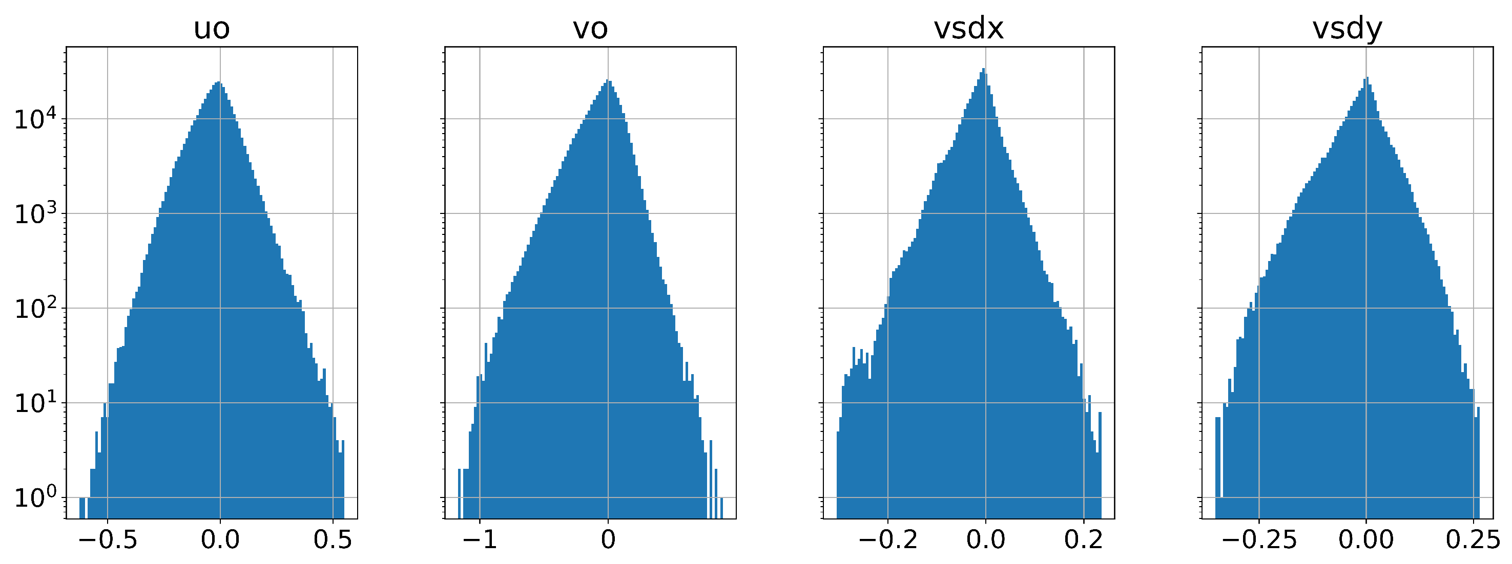
One key aspect when analysing time series is related to the series stationarity, which, in our case, is seasonal stationarity for the vector components of wind and wave data. The first step is to perform the augmented Dickey-Fuller test upon the dataset but this test provides
p-values strictly less than
, as all of them (as seen in
Table 2), we plotted the histograms clearly showing the stationary Gauss form (see
Figure 3).
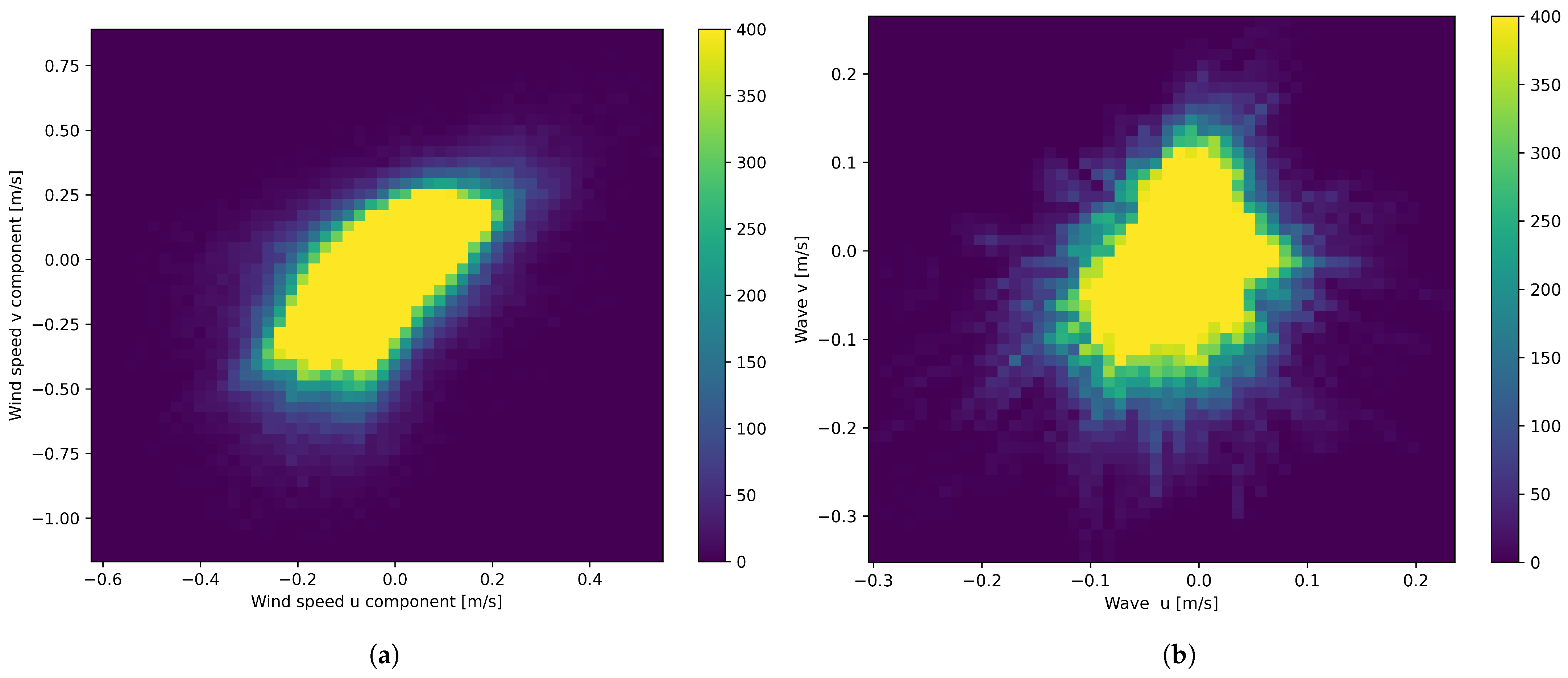
The orthogonal vector representation for geospatial data allows us to perform several analyses, thus enabling a more comprehensible view of the system dynamics. The first data quality check is performed using the correlation between wind and wave orthogonal components (as shown in
Figure 4), where the expected influence between these two parameters is visible.
During the implementation, we found one issue with TFT models, which is related to the fact that it cannot handle both positive and negative values within the time-series, leading us to increment the vector values with a static value of 2. This greatly improves the model convergence towards our implementation.
Figure 3 and
Figure 4a,b present a visual representation of wind and wave data, showcasing intriguing patterns and correlations. Both wind and wave data exhibit a clustering of points around the origin, indicating a prevalence of lower magnitudes.
Both
Figure 4a,b show a high concentration of data points around the origin (0, 0) and exhibit an elliptical shape, suggesting a potential correlation between the U and V components. However, the wind speed distribution in
Figure 4a appears more dispersed than the wave component distribution in
Figure 4b, indicating a wider range of magnitudes and directions. This observation suggests that wind patterns exhibit greater variability than wave patterns, potentially reflecting the influence of atmospheric conditions on wind dynamics. Additionally, as is pointed out in [
38], the wind and wave data exhibit similar trends throughout the year. The winter months show higher wind speeds and wave heights, while the summer months show lower values. This seasonal variation is consistent with the general understanding of the Black Sea’s climate and its influence on wind and wave patterns [
38].
2.2. Temporal Fusion Transformer (TFT) Architecture
Simple Recurrent Layer time series prediction models, often employed in the literature, fail to fully capture the intricacies of the modelled system. Both single-step and multi-step window models exhibit suboptimal predictive quality. We aim to predict wave components using highly reliable data sources, such as Copernicus Marine Environment Monitoring Service (CMEMS), enabling researchers to estimate input data for diffusion models accurately before it becomes available. This application is vital for analyzing incidents involving pollutants or floating devices in the Black Sea environment. We identified the TFT framework as the most accurate architecture for this task [
39]. Our implementation utilizes PyTorch [
40], chosen for its user-friendliness and diagnostic tools, facilitating the development of white-box models [
41] with explainable AI through interpretability features [
42]. While metaparameter tuning can be computationally expensive, PyTorch offers a dedicated training pipeline through PyTorch Lightning [
35]. The training pipeline splits the data into training and testing using 388,598 records of the data for training and 1100 records for validation. Validation data is not seen during the training and is performed for the diagnostic and explanation plots. This provides estimated starting points for essential parameters, including the initial learning rate, significantly expediting model convergence.
Hyperparameter optimization is conducted using Optuna utils [
43] with the search ranges detailed in
Table 3.
To optimize model training, we integrated a learning rate normalizer and an early-stopping callback function. This function terminates training if no improvement is detected for 10 consecutive epochs, enhancing efficiency and mitigating potential overfitting.
While our work focuses upon 4 components, two for windspeed (x component denoted by
uo and the y component denoted by
vo) and the other two for the wave (the x component denoted by
vsdx and the y component denoted by
vsdy) we have built 4 distinct models for each of those. Each model has its hyperparameter search (within the same search value values from
Table 3) and provides different best model results presented in
Table 4.
3. Results and Discussion
This section presents the findings on predicting coastal dynamics along the Western Black Sea coast using a combination of in-situ and modelled marine data. We first described the dataset and preprocessing steps (
Section 2.1), followed by the model development and evaluation. Finally, we discuss the key findings and their implications for coastal dynamics prediction.
3.1. Data Exploration
In
Figure 4a,b, the highest concentration of wave component data points is clustered around the origin (0, 0), indicating a predominance of low magnitudes. The distribution exhibits an elliptical shape, suggesting a potential correlation between the U and V components. This elongation along the diagonal implies a tendency for both components to have the same sign, expressing a consistent wave direction. Comparing the two figures reveals similarities in the overall shape and concentration of data points around the origin. However, the wind speed distribution in
Figure 4a appears more dispersed than the wave component distribution in
Figure 4b. This suggests that wind speeds exhibit a wider range of magnitudes and directions compared to the wave components. These visualizations provide valuable insights into the interrelationships between wave and wind data’s U and V components, highlighting their typical magnitudes and directional tendencies. Further analysis, such as calculating correlation coefficients or fitting multivariate distributions, could quantify these relationships and better characterise both wind and wave dynamics.
3.2. Model Interpretability
The integrated interpretable AI provided us with insights into model prediction importance attribution upon the input parameters and model architecture. Recent developments led to implementing the Interpretable Multihead Attention mechanism providing us with key insights on how to model led to the required prediction.
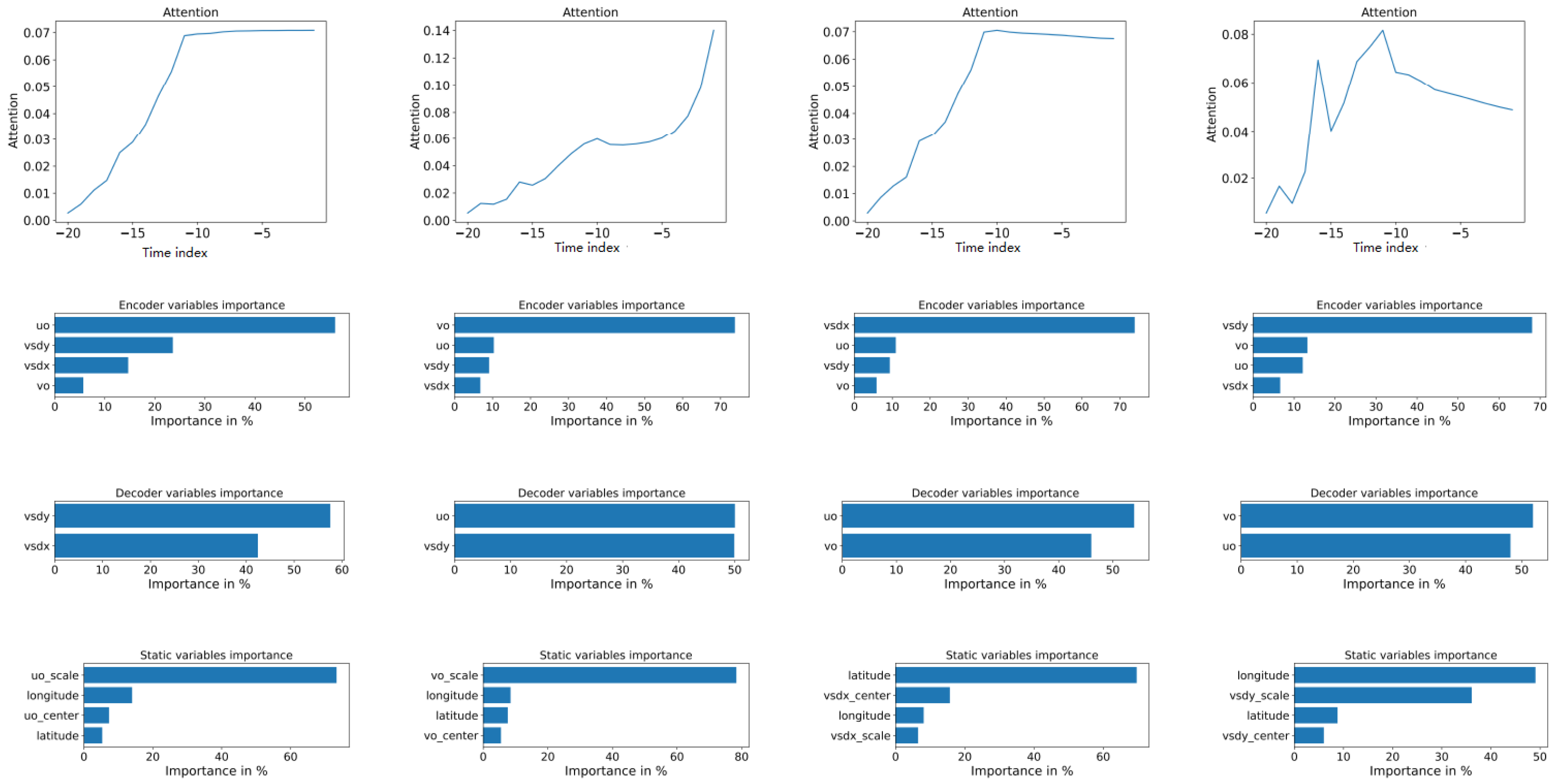
Figure 5 provides a sample for the implementation of such an attention mechanism.
The implemented models consider the previous 15 days of data (one datapoint per day) shown as negative values in
Figure 5. For the
uo model, the most influential parameter is related to the static scale factor (approx. 70%) and its previous values (approx. 55%). While creating the output, in the
Decoder layer, the most influential parameter is the orthogonal value of
vsdy (approx. 57%). While the wind wide-spawn shows lesser dependence upon the position (latitude and longitude), the values require less normalization by the orthogonal
vo variable.
For the second wind component
vo from
Figure 5 (second column from left to right), it seems that this is the most dominant component of the Black Sea system as its major dependencies are related to its own scale (Static variables) and previous values (encoder variables). At the same time, the decoder shows 50/50 dependence between the y component of the wave (
vsdy) and the orthogonal value for wind (
uo). The attention plot also suggests that the model focuses more on closer previous values than the other analyzed components that focus on more than the most recent values for the same component.
The later components vsdx and vsdy refer to wave data that tends to have more inertia as previous values are considered for a larger interval. The x component (vsdx shows a stronger dependency upon the latitude (approx. 70%) followed by its previous values (within the encoder) (approx. 74%). At the same time, the decoder focuses on wind components (the uo—similar direction), which is more important than the orthogonal wind vector—vo.
The y component (
vsdy—the last column in
Figure 5) shows a higher dependency upon the
longitude (approx. 48%) and its previous values (approx. 68%). The decoder variables show a dependence on
vo (approx. 52% than
uo—approx. 48%).
The component ‘uo’ represents the wind speed’s x-component. The model predicting ‘uo’ relies heavily on a static scale factor (about 70%) and its past values (around 55%). Interestingly, when generating the output, the most influential parameter becomes the y-component of the wave data (vsdy), contributing approximately 57%. This suggests a complex interplay between wind and wave patterns where recent wave behaviour in the y-direction significantly influences the wind in the x-direction.
The component vo, the wind speed’s y-component, seems a dominant factor in the Black Sea system, as the model primarily depends on its scale (static variables) and previous values (encoder variables). The output depends equally on the y-component of the wave (vsdy) and the x-component of the wind (uo). Notably, the model for ‘vo’ focuses more on recent past values than the other components, which consider a wider range of historical data.
The component vsdx represents the x-component of wave data. It strongly depends on latitude (around 70%) and its past values (approximately 74%). The output is primarily influenced by the wind components, particularly ‘uo’, aligning with the general understanding that wind direction significantly impacts wave direction.
Lastly, vsdy is the y-component of wave data. It depends strongly on longitude (about 48%) and its past values (around 68%). The output is more influenced by vo (about 52%) than ‘uo’ (approximately 48%).
3.3. Accuracy and Robustness of the TFT Model
A model accuracy and robustness test was performed during the training stage for each of the 4 models implemented within this article. The results are presented in
Table 5.
Early stopping mechanisms provided consistent training time reduction, while using smaller patience (20 epochs) should stop the training process if no improvement was achieved for the fourth decimal of the loss value. This is appropriate for situations where smaller models are required, while it provides us with information about the model’s complexity. While hyper-parameter tuning methods provide us with the smaller fit model for the problem at hand, when early stopping is triggered after a small epoch count (usually less than 50%—in our case, 50% of target 200 epochs is 100 epochs), it means that the model needs a larger block size to correctly fit the problem.
3.4. Model Performance
Figure 6,
Figure 7,
Figure 8 and
Figure 9 examine the predictive capabilities of the TFTs model for coastal dynamics along the Western Black Sea coast. It presents a multi-variate time series prediction, demonstrating the model’s ability to forecast a specific component of coastal dynamics, potentially the U or V component of the wind or sea wave, over a 15-day period. The x-axis represents the reference time in days, while the y-axis indicates the magnitude of the predicted component. The blue line depicts the model’s predictions, while the green dots represent the observed values. The close alignment between the predictions and the observed values indicates the model’s high accuracy in capturing the temporal dynamics of coastal currents. The figures also highlights the model’s effectiveness in handling long-term dependencies and complex non-linear relationships inherent in the data.
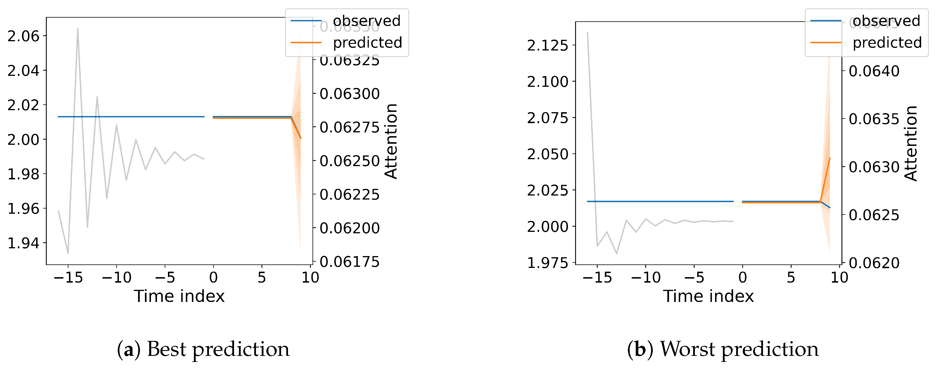
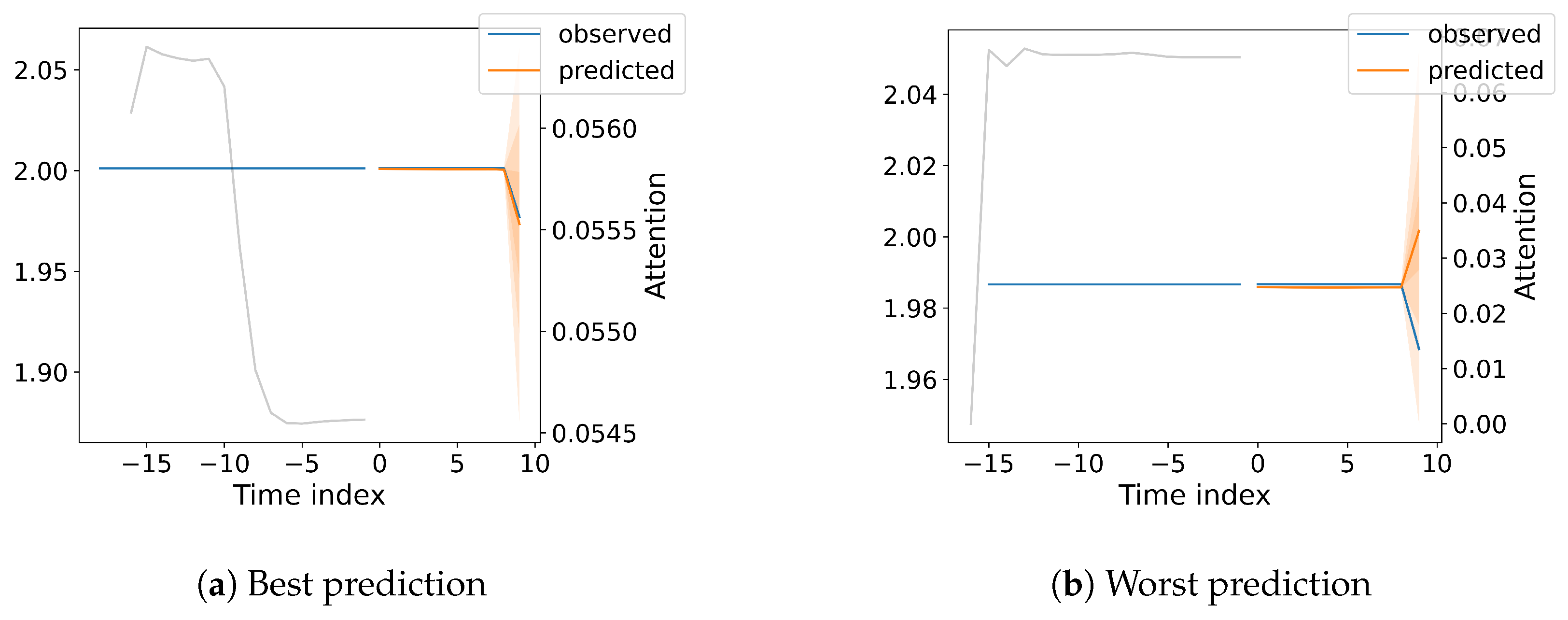
Prediction accuracy is estimated with a random sample of 10 records from the testing dataset for each implemented method. For diagnostic purposes, we also plotted the attention (with a grey line). The prediction is shown in yellow and the actual value is represented in blue. One major improvement for the TFT model is introduced with the QuantileLoss function that estimates the model confidence level upon the actual predicted value and informs the user about the associated probability. The Quantile Loss is illustrated with different levels of shaded red (the intensity of the red area is directly related to the associated quantile).
Within the figures mentioned, the predicted component value (incremented by 2) is denoted on the left scale, while we present the Attention value on the right scale.
Figure 6 provides valuable insights into the TFT model’s temporal attention mechanism and its ability to adapt to different scenarios in predicting coastal dynamics. The close alignment between the observed (blue) and predicted (orange) values demonstrates the model’s accuracy in forecasting the U component of wind on coastal stations. This supports the findings in your paper regarding the TFT model’s strong predictive performance. This also proves that our scaling factor does not influence the predicted values. The most noticeable difference lies in the attention patterns. In
Figure 6a, the model focuses primarily on a past time step around −15, suggesting a potential lag effect or recurring pattern in the data. In contrast,
Figure 6b shows a more distributed attention pattern with a peak around −5, indicating that a broader range of recent past time steps influences the current prediction.
This difference in attention patterns highlights the model’s ability to adapt its focus based on the specific dynamics of the data. It suggests that the TFT model can identify and utilize relevant historical information, whether it’s a specific past event (
Figure 6a) or a combination of recent trends (
Figure 6b).
Figure 7a,b shows a gradual increase in attention towards the hindcast, culminating in a sharp peak at the most recent time step. This suggests the model is capturing an evolving trend in the data. In contrast,
Figure 7a focuses almost exclusively on the most recent time step, indicating that the immediate past is the dominant factor influencing the prediction in this scenario. The observed values in
Figure 7a exhibit a gradual upward trend, while
Figure 7b shows an abrupt, steep drop towards the end. This difference in data dynamics highlights the model’s ability to adapt its attention mechanism to capture various temporal patterns, whether gradual or abrupt.
The strongest component presented in
Figure 7 related to the N-S wind movement also provides accurate results, the worst results show a difference of 0.35 from the predicted value, within acceptable levels. The quantile loss shows that improvements are possible.
In
Figure 8a, a gradual increase in attention towards the recent past can be observed, culminating in a sharp peak at the most recent time step (−11). This suggests the model is capturing an evolving trend while also being highly responsive to immediate changes. In contrast,
Figure 8b shows evenly distributed attention across the hindcast steps, indicating that a broader historical context influences the current prediction. The difference in attention patterns is likely related to the different dynamics observed in the data.
Figure 8a shows a gradual upward trend in the observed values, while
Figure 8b exhibits a relatively stable pattern. The model adapts its attention accordingly, focusing on the most relevant time steps for each scenario.
Figure 9a shows a distinct peak in attention around −14 time steps in the past, indicating that this particular historical data point is highly influential in predicting the current value. In contrast,
Figure 9b shows a more gradual decline in attention weights, with a slight peak around −15 time steps and a more pronounced peak towards the very recent past (hindcast). The observed values in
Figure 9a exhibit a relatively stable pattern, while
Figure 9b shows a slight upward trend with a steeper increase towards the end. This difference in data dynamics highlights the model’s ability to adapt its attention mechanism to capture various temporal patterns, including scenarios where long-term dependencies play a significant role.
The close correspondence between the model’s predictions and in-situ observations highlights its strong accuracy in capturing the temporal dynamics of coastal dynamics. This accuracy is further substantiated by the interpretability features of TFTs, which enable the identification of the most influential input variables in the predictions, such as wind and wave measurements. These insights reveal the mechanisms behind the underlying physical processes driving coastal dynamics.
Figure 6,
Figure 7,
Figure 8 and
Figure 9 also emphasize the model’s capability to handle long-term dependencies and complex non-linear relationships inherent in the data.
The TFT model’s attention mechanism reveals challenging insights into the dynamics of coastal currents along the Western Black Sea coast. The model’s focus on specific historical time steps varies significantly across different scenarios and components. For instance, in predicting the U component of wind, the model sometimes focuses on a distant past time step (around −15), suggesting a potential lag effect or recurring pattern in the data. In other cases, the attention is more evenly distributed, indicating that a broader range of recent past time steps influences the current prediction. This adaptive attention is also evident in predicting the V component. When the observed values exhibit a gradual upward trend, the model’s attention gradually increases towards the most recent time step, suggesting that it captures an evolving trend. However, when there’s an abrupt drop in the observed values, the model focuses almost exclusively on the most recent time step, indicating that the immediate past dominates the prediction. These observations suggest that the TFT model can effectively identify and utilize relevant historical information, whether it’s a specific past event, a combination of recent trends, or a long-term dependency. This adaptability highlights the potential of TFTs in capturing the complex temporal dynamics inherent in coastal current data, ultimately leading to more accurate and insightful predictions.
4. Discussion
Recent advancements in Explainable AI (XAI) have significantly impacted various fields, including meteorology and oceanography, particularly through the application of TFTs. TFTs are designed to handle multi-horizon time series forecasting, which is significant for predicting meteorological phenomena such as wind and wave patterns. The architecture of TFTs integrates attention mechanisms that allow for the interpretation of model predictions, making them particularly suitable for applications where understanding the underlying decision-making process is essential.
The foundational work on TFTs by Lim et al. introduced an attention-based architecture that not only enhances forecasting accuracy but also provides interpretable insights into the model’s predictions [
39]. This is particularly relevant in meteorological applications where stakeholders need to understand the factors influencing predictions, such as atmospheric conditions and historical data trends. The model’s ability to incorporate various input types and temporal relationships allows it to adapt to the complexities of meteorological data, which often includes non-linear interactions and varying temporal resolutions [
39].
In the context of meteorology, TFTs have been employed to forecast wind speeds and wave heights, which are critical for maritime operations and coastal management. For instance, Luo et al. proposed a variant of the TFT, TFTOps, tailored explicitly for anomaly detection in operational contexts, which can be beneficial for identifying unusual weather patterns that may affect wind and wave forecasts [
44]. The fusion of probabilistic inputs in TFTOps enhances its robustness, allowing for better handling of uncertainties inherent in meteorological data [
44].
Moreover, the application of TFTs extends beyond common forecasting. They have been utilized in the analysis of high-resolution wind fields, as demonstrated by Schlager et al., who developed a diagnostic application that leverages dense meteorological station networks to generate real-time wind field data [
45]. This application exemplifies how TFTs can facilitate the integration of diverse data sources, improving the spatial and temporal resolution of wind forecasts, which is essential for accurate maritime navigation and safety.
The interpretability of TFTs is further enhanced by their ability to provide insights into the temporal dynamics of the data. For example, the work by Burrichter on forecasting sewer overflow during pluvial flash floods utilized TFTs to predict overflow hydrographs at a granular level, demonstrating the model’s capability to handle complex, time-dependent phenomena [
46]. This level of detail is determinative in meteorology and oceanography, where understanding the timing and magnitude of events can inform decision-making processes.
In addition to their forecasting capabilities, TFTs have been integrated into frameworks that combine multiple data sources for enhanced meteorological predictions. For instance, Wang et al. explored the integration of multi-dimensional meteorological information using spatio-temporal fusion techniques, which align well with the capabilities of TFTs to process and analyze complex datasets [
47]. This approach not only improves the accuracy of forecasts but also provides a more comprehensive understanding of the interactions between different meteorological variables.
The application of TFTs in oceanography is also noteworthy, particularly in the context of wave forecasting. The ability to model long-range dependencies and capture temporal relationships is essential for predicting wave patterns, which are influenced by many factors, including wind speed, direction, and atmospheric pressure. The integration of TFTs into oceanographic models can enhance the accuracy of wave forecasts, thereby supporting maritime operations and coastal management strategies.
Recent work by Tedesco highlights the application of neural networks for bias correction in operational storm surge forecasts, demonstrating that machine learning can effectively enhance the accuracy of predictions in complex marine environments [
48]. This study is a foundational reference for understanding how neural networks can be utilized to correct systematic errors in traditional forecasting models. The findings indicate that by integrating observational data with model outputs, the performance of storm surge forecasts can be significantly improved, which is particularly relevant for the Romanian Black Sea context, where various atmospheric and oceanographic factors influence coastal dynamics.
Similarly, the research conducted by Bajo and Umgiesser explores the synergy between dynamic models and neural networks for storm surge forecasting [
49]. Their findings suggest that a hybrid approach, combining both methodologies’ strengthswhich combines the strengths of both methodologies, can lead to more accurate and reliable predictions. This aligns with the overarching theme of this literature review, which posits that integrating multiple data sources—whether observational or modelled—can enhance the predictive capabilities of coastal dynamics models. The study emphasizes the importance of data assimilation practices, which are critical for improving the accuracy of forecasts in non-linear environments, such as those encountered in coastal regions.
Furthermore, ongoing research into enhancing the capabilities of TFTs continues to produce promising results. For example, the development of hybrid models that combine TFTs with other machine learning techniques is being explored to improve forecasting performance and interoperability [
50]. These advancements are essential for addressing the challenges posed by meteorological and oceanographic data’s dynamic and complex nature.
Recent research in the Black Sea region has increasingly focused on the integration of artificial intelligence (AI), machine learning (ML), and explainable AI (XAI) within the context of oceanography, particularly through the CMEMS [
1]. This synthesis highlights the advancements and applications of these technologies in understanding marine ecosystems, monitoring biogeochemical processes, and enhancing predictive capabilities. One significant area of research involves the application of Bayesian networks to analyze the complex structure of marine ecosystems in the Black Sea. Krivoguz et al. utilized CMEMS environmental datasets, incorporating variables such as sea surface temperature, salinity, and nutrient concentrations, to model the interactions within these ecosystems effectively [
51]. This approach underscores the potential of AI methodologies to resolve the intricate dynamics of marine environments, which are often characterized by their multiparametric nature. Moreover, the CMEMS has been pivotal in developing operational services for monitoring and forecasting ocean states in the Black Sea. Ciliberti et al. highlighted recent advancements in the CMEMS, which have facilitated the integration of AI techniques for real-time data analysis and forecasting biogeochemical processes [
52].
Regarding specific machine learning applications, several studies have illustrated their effectiveness in predicting ocean phenomena and managing marine resources. For instance, Hafez discussed various ML algorithms that have been employed for tasks such as habitat modelling, species identification, and pollution detection [
53]. Similarly, Xu et al. reviewed the use of AI tools for identifying and forecasting oceanic events, such as oil spills and algal blooms, which are critical for environmental monitoring and management [
54]. These applications highlight AI and ML’s transformative potential in addressing pressing oceanography challenges. The development of the Black Sea Reanalysis System within CMEMS further exemplifies the integration of advanced computational techniques in oceanographic research. Lima et al. described how this system employs variational data assimilation methods to combine observational data with ocean circulation models, providing a comprehensive overview of the Black Sea’s state over time [
55]. Such reanalyses are essential for understanding long-term climatic trends and their impacts on marine ecosystems.
Additionally, the role of AI in enhancing the accuracy of oceanographic predictions cannot be overstated. Recent studies, such as those by Sonnewald et al., have demonstrated how machine learning can bridge observational data and theoretical models, thereby improving the understanding of ocean dynamics [
56]. This integration of AI not only accelerates research but also opens new avenues for empirical analysis within the field.
5. Conclusions
This study demonstrates the significant potential of TFTs for advancing both predictive accuracy and interpretability in the field of coastal dynamics. By successfully integrating in-situ observations with modelled data from the Copernicus Marine Service, this research highlights the capacity of TFTs to not only generate precise forecasts of U and V current components along the Western Black Sea coast but also to provide valuable insights into the underlying physical processes driving these dynamics. The model’s ability to effectively capture complex temporal dependencies and non-linear relationships within the data underscores its potential for enhancing our understanding of coastal processes and contributing to more effective marine resource management and conservation strategies. As the field evolves, integrating TFTs with other data sources and machine-learning techniques will likely lead to even more robust and insightful models, further refining our understanding of complex marine systems.
Our initial working hypotheses revolved around the potential of TFTs to enhance the prediction of coastal dynamics along the Western Black Sea coast. We postulated that TFTs, with their ability to handle complex temporal dependencies and incorporate both static and time-varying features, would outperform traditional methods and provide valuable insights into the underlying physical processes. Our results strongly support these hypotheses. The TFT model demonstrated high accuracy in predicting the U and V components of both wind and wave currents, surpassing the performance of simpler recurrent layer models. The model’s ability to capture the complex non-linear relationships and long-term dependencies in the data is evident in its close alignment with observed values. Furthermore, the interpretability features of TFTs allowed us to identify the most influential input variables and gain a deeper understanding of the factors driving coastal dynamics. The attention mechanism, in particular, revealed how the model’s focus on specific historical time steps varied across different scenarios and components, highlighting potential lag effects, recurring patterns, and evolving trends in the coastal dynamics data. An unexpected finding was the model’s ability to adapt its attention based on the specific dynamics of the data. For instance, in predicting the V component of wind, the model focused on a distant past time step when there was a gradual upward trend in the observed values, while it concentrated on the most recent time step when there was an abrupt drop. This adaptability suggests that TFTs can effectively discern and utilize relevant historical information, leading to more accurate and insightful predictions. These findings have significant implications for understanding coastal processes in the Black Sea. The TFT model’s ability to accurately predict and interpret coastal dynamics could enhance our understanding of the complex interactions between atmospheric conditions, wave patterns, and coastal currents. This knowledge could contribute to more effective marine resource management and conservation strategies, as well as improved maritime safety.
In the context of our Black Sea wave prediction study, the TFT model’s ability to handle complex temporal dependencies was demonstrated by its high accuracy in forecasting the U and V components of wave currents over a 30-day period. This accuracy is evident in the close alignment between the model’s predictions and the observed values, as depicted in
Figure 6,
Figure 7,
Figure 8 and
Figure 9. The model effectively captured the temporal dynamics of coastal currents, including long-term dependencies and complex non-linear relationships inherent in the data. This capability is particularly important in the Black Sea region, where coastal dynamics are influenced by a complex interplay of atmospheric conditions, wave patterns, and coastal currents.
Compared to previous studies using other AI/ML techniques or traditional methods for coastal dynamics prediction, our TFT model demonstrates significant advancements in the Black Sea region. The model’s superior accuracy in capturing complex temporal dependencies and non-linear relationships highlights its potential for enhancing the prediction of coastal dynamics. Additionally, the interpretability features of TFTs provide valuable insights into the underlying physical processes, surpassing the capabilities of traditional black-box AI/ML models.
Our study has certain limitations, such as the specific region and time period considered. Future research could expand on these aspects by incorporating additional data sources, such as sea surface temperature, salinity, and atmospheric pressure, to potentially further improve prediction accuracy. Additionally, exploring the model’s performance in different seasons and under varying hydrometeorological conditions could provide valuable findings. Applying the developed methodology to other coastal regions could also contribute to a broader understanding of the applicability and generalizability of AI/ML techniques in predicting coastal dynamics.


