Article

An Improved Adaptive Robust Extended Kalman Filter for Arctic Shipborne Tightly Coupled GNSS/INS Navigation

1
Merchant Marine College, Shanghai Maritime University, Shanghai 201306, China
2
College of Engineering Science and Technology, Shanghai Ocean University, Shanghai 201306, China
3
Shanghai Ship and Shipping Research Institute, Shanghai 200135, China
*
Author to whom correspondence should be addressed.
J. Mar. Sci. Eng. 2025, 13(12), 2395; https://doi.org/10.3390/jmse13122395
Submission received: 19 November 2025 / Revised: 9 December 2025 / Accepted: 13 December 2025 / Published: 17 December 2025
(This article belongs to the Section Ocean Engineering)

Abstract

In the Arctic region, the navigation and positioning accuracy of shipborne and autonomous underwater vehicle (AUV) integrated Global Navigation Satellite System (GNSS) and Inertial Navigation System (INS) solutions is severely degraded due to poor satellite geometry, frequent ionospheric disturbances, non-Gaussian measurement noise, and strong multipath effects, as well as long-term INS-based dead-reckoning for AUVs when GNSS is unavailable underwater. In addition, the sparse ground-based augmentation infrastructure and the lack of reliable reference trajectories and dedicated test ranges in polar waters hinder the validation and performance assessment of existing marine navigation systems, further complicating the achievement of accurate and reliable navigation in this region. To improve the positioning accuracy of the GNSS/INS shipborne navigation system, this paper adopts a tightly coupled GNSS/INS navigation approach. To further enhance the accuracy and robustness of tightly coupled GNSS/INS positioning, this paper proposes an improved Adaptive Robust Extended Kalman Filter (IAREKF) algorithm to effectively suppress the effects of gross errors and non-Gaussian noise, thereby significantly enhancing the system’s robustness and positioning accuracy. First, the residuals and Mahalanobis distance are calculated using the Adaptive Robust Extended Kalman Filter (AREKF), and the chi-square test is used to assess the anomalies of the observations. Subsequently, the observation noise covariance matrix is dynamically adjusted to improve the filter’s anti-interference capability in the complex Arctic environment. However, the state estimation accuracy of AREKF is still affected by GNSS signal degradation, leading to a decrease in navigation and positioning accuracy. To further improve the robustness and positioning accuracy of the filter, this paper introduces a sliding window mechanism, which dynamically adjusts the observation noise covariance matrix using historical residual information, thereby effectively improving the system’s stability in harsh environments. Field experiments conducted on an Arctic survey vessel demonstrate that the proposed improved adaptive robust extended Kalman filter significantly enhances the robustness and accuracy of Arctic integrated navigation. In the Arctic voyages at latitudes 80.3° and 85.7°, compared to the Loosely coupled EKF, the proposed method reduced the horizontal root mean square error by 61.78% and 21.7%, respectively.

1. Introduction

As the Arctic ice cap melts year by year due to global warming, the Arctic is gradually meeting the conditions for navigation. With the improvement of the navigation capacity of the Arctic shipping route, the strategic importance of the Arctic shipping route in global maritime traffic is becoming more and more apparent [1,2]. The Arctic shipping route is located in a region with frequent global economic activities and important strategic position. Its strategic value in global shipping, energy development, scientific research and exploration is increasing, and polar activities are therefore becoming more frequent [3,4]. In addition to merchant and research vessels, autonomous underwater vehicles (AUVs) are now widely deployed in polar waters for under-ice surveys, seabed mapping, resource exploration, and environmental monitoring, which further increases the demand for high-precision and high-reliability navigation in this region. Navigation systems thus play a key role in ensuring the safety of polar shipping, supporting AUV operations, and promoting polar development, and their reliability and accuracy in the polar environment are crucial. However, navigation systems in the mid-to-high latitudes of the Arctic face severe challenges. GNSS signals usually appear at low elevation angles, which leads to the degradation of satellite geometry and an increase in the geometric dilution of precision (GDOP). In addition, phenomena such as ionospheric disturbance, signal scintillation, multipath effects, and cycle slips occur frequently in this region, which seriously limit the adaptability and performance of traditional navigation methods in this environment [5,6]. For AUVs operating beneath sea ice, GNSS signals are unavailable for most of the mission, so the vehicles must rely mainly on INS, Doppler velocity logs, and acoustic positioning systems; as a result, long-duration under-ice missions are prone to rapid error accumulation and performance degradation under complex polar conditions. Furthermore, in high-latitude regions, the gyroscopes and accelerometers of inertial measurement units (IMUs) are affected by additional error sources, including amplification of the Coriolis effect caused by the Earth’s rotation, mismatch of local gravity models, and coordinate singularities caused by meridian convergence. These effects weaken the effectiveness of the gravity vector-rotation vector constraints used in the attitude alignment stage of traditional inertial navigation systems, causing attitude solutions and inertial errors to increase rapidly with increasing latitude. To mitigate this problem, free-orientation, roaming-orientation, and normal-vector mechanical arrangement schemes based on grid navigation coordinate systems have been proposed to alleviate the effects of high-latitude singularities [7,8,9,10,11]. How to improve the positioning accuracy and robustness of shipborne and AUV navigation systems in the Arctic region has therefore become a critical issue that urgently needs to be addressed [12,13,14].
GNSS/INS integrated navigation systems are widely used due to their complementarity [15,16,17,18]. The advantages of GNSS and INS respectively enable their integration to give full play to their respective strengths, playing a crucial role in improving positioning accuracy and reliability, and becoming a key technical means to meet the positioning needs of various application scenarios. GNSS/INS integration is generally divided into two modes: loose coupling and tight coupling. The loose coupling method performs data fusion based on the complete GNSS positioning solution, but it cannot provide effective positioning when there are fewer than four available satellites. In contrast, the tight coupling method directly combines the original measurement results of the global navigation satellite system with the output of the inertial navigation system, thereby making more effective use of some satellite data [19,20,21]. This method greatly improves positioning accuracy and robustness, especially in complex urban environments [22,23].
GNSS/INS integrated navigation typically employs a Kalman filter (KF) for state estimation and error correction. KF is a recursive optimal estimation algorithm based on the minimum mean square error (MMSE) criterion. Due to its ability to effectively handle random noise and uncertainty, it is widely used in dynamic state estimation in GNSS/INS integrated navigation systems [24,25]. However, GNSS signals are susceptible to interference from the external environment [26,27,28,29], and this problem is particularly prominent in polar environments. Poor satellite geometry and frequent ionospheric disturbances often cause global navigation satellite system observations to be affected by outliers. These outliers usually exhibit significant discrete deviations and typically follow a non-Gaussian heavy-tailed noise distribution [30,31,32]. Such anomalous observations violate the basic assumption of KF regarding Gaussian noise, thereby reducing the accuracy of state estimation and, in severe cases, causing filter divergence [33]. For shipborne platforms operating in complex polar environments, stable and accurate navigation information is crucial. Therefore, there is an urgent need to design a more robust filtering method to improve the state estimation accuracy and overall performance of shipborne navigation systems in the Arctic navigation area.
To address the problem that KF cannot effectively handle nonlinear noise in complex dynamic environments, researchers have proposed a variety of nonlinear filtering methods to improve positioning accuracy. For this purpose, Kalman and Bucy [34] proposed the Extended Kalman Filter (EKF), which expands the nonlinear function based on KF and ignores higher-order terms to handle nonlinear problems. EKF performs well in general nonlinear problems and has a small computational cost, so it has been widely used. Other scholars have proposed unscented Kalman filter (UKF) [35], cubature Kalman filter (CKF) [36,37] and particle filter (PF) [38], which can also effectively solve nonlinear problems and improve the accuracy of state estimation. In addition to nonlinear problems, modeling error and time-varying noise statistics are still the main problems in complex environments. In addition, outliers in measurements are usually unpredictable and unavoidable, which may lead to a significant increase in estimation error or even filter divergence. In recent years, Adaptive Kalman Filter (AKF) and Robust Kalman Filter (RKF) have received much attention due to their high accuracy and robustness. AKF has great potential in dealing with uncertain models and time-varying noise, mainly by adjusting the filtering parameters in the innovation sequence to optimize the estimation. Although different AKF methods differ in implementation, their common goal is to redistribute the weights of the predicted state and the observation in the state estimation by adjusting the Kalman gain. Some scholars have proposed an adaptive Kalman filter (AKF) [39] to improve the robustness of the state estimation by estimating the noise covariance online. The adaptive robust Kalman filter (ARKF) proposed by Kai Shen et al. [40] has made an adaptive robust improvement to the Kalman filter (KF) by introducing a new adaptive factor, which can adjust the estimation error covariance matrix and the Kalman gain according to the actual process, thereby improving the adaptability and positioning accuracy of the filter. Recently, Taewon Uhm et al. [41] proposed the Adaptive Robust Extended Kalman Filter (AREKF). Based on EKF, a robust factor is introduced to suppress the influence of measurement outliers on the filtering performance. Combined with an adaptive factor based on innovative residuals and posterior residuals, the covariance of process noise and measurement noise is estimated and adjusted online, thereby dynamically optimizing the Kalman gain and taking into account both the robustness and adaptability of the filter. In addition, Chun Ma et al. [42] proposed an improved multiple-outlier-robust Kalman filter (I-MORKF) based on a bifactor robust estimation framework, which enhances the robustness and accuracy of the traditional MORKF under non-Gaussian noise and gross measurement errors.
The above studies have been very inspiring to us. Building upon existing research on the Adaptive Robust Extended Kalman Filter (AREKF), we aim to mitigate the impact of challenging environmental factors unique to the Arctic region, such as sparse satellite numbers, poor satellite geometry, and low satellite elevation angles. Previous research has primarily focused on improving the performance of the AREKF algorithm in conventional environments, while the Arctic region presents unique challenges requiring a more robust solution. Therefore, we propose an improved AREKF algorithm based on the sliding window technique. This method dynamically adjusts the observation noise covariance, effectively reducing the impact of environmental noise and transient disturbances on navigation results. By introducing this technique, we enhance the robustness of the shipborne navigation system.
The main contributions of this paper are as follows:
(1)
Establishing a Tightly Coupled GNSS/INS Mathematical Model: This paper first establishes a mathematical model for tightly coupled GNSS/INS integrated navigation and further analyzes the accuracy differences between loosely coupled and tightly coupled models in practical applications. Through processing and analysis of actual Arctic navigation data, the navigation accuracy performance of the two combined methods is explored in depth. Research shows that the tightly coupled model can more effectively integrate GNSS and INS data compared to the loosely coupled model, improving the system’s navigation accuracy and robustness, especially in complex environments. Comparative experiments further verify the advantages of tightly coupled integrated navigation under extreme navigation conditions.
(2)
Extended Kalman Filter Optimization: To address the degradation problem of Arctic GNSS signals, this paper first replaces the traditional Extended Kalman Filter (EKF) with an Adaptive Robust Extended Kalman Filter (AREKF) based on Mahalanobis distance. By calculating the Mahalanobis distance of the residuals and comparing it with a set chi-square threshold, the innovative covariance matrix is dynamically adjusted. Furthermore, a sliding window-based observation noise covariance matrix estimation framework is used to further improve the system’s robustness and estimation accuracy under GNSS signal anomalies.
(3)
Arctic Shipborne Data Validation: To verify the effectiveness and robustness of the proposed method, this paper validated it using real Arctic shipborne data, covering two continuous trajectories of approximately 1300 s at latitudes of 80.3° and 85.7°. In the test at latitude 80.3°, the horizontal positioning accuracy was improved by 61.78% compared to the traditional method; in the test at latitude 85.7°, the horizontal positioning accuracy was improved by 21.7%. Experimental results show that under extreme conditions of severe GNSS signal degradation, the proposed method can effectively maintain excellent horizontal accuracy and robustness.
The remainder of this paper is arranged as follows: Section 2 introduces the GNSS/INS tightly coupled system model and the principles and execution process of the IAREKF algorithm. Section 3 introduces the shipborne experimental setup in the Arctic, including sensor configuration and data collection on the Xue Long 2 icebreaker. Section 4 experimentally verifies the proposed IAREKF algorithm and evaluates its effectiveness. Section 5 summarizes the entire paper and looks forward to future research directions.

2. System Model and Filtering Algorithm

This study considers the influence of other error sources in gyroscope and accelerometer measurements in the mid-to-high latitudes of the Arctic and mitigates these effects by employing a normal-vector-based inertial mechanical orchestration method. Furthermore, to address the complex navigation challenges in the Arctic region, this paper adopts a tightly coupled GNSS/INS combination and proposes an improved Adaptive Robust Extended Kalman Filter (IAREKF) algorithm. This method combines the advantages of Mahalanobis distance and chi-square test, proposing a sliding window-based framework to estimate the observation noise covariance matrix. The algorithm dynamically adjusts the observation noise covariance matrix, enhancing its robustness to outliers and non-Gaussian noise. Moreover, to eliminate the impact of residual inconsistencies on integrated navigation, this paper introduces the mean and standard deviation of the sliding window historical residuals, aiming to cope with constantly changing environmental conditions and enhance the robustness of the filter.
This chapter mainly introduces some algorithms and models used in this paper, including the basic principles and execution process of the GNSS/INS tightly coupled integrated navigation system model, the extended Kalman filter (EKF), and the improved adaptive robust extended Kalman filter (IAREKF).

2.1. Common Part of GNSS/INS Dynamic Model

The error states in GNSS/INS integrated navigation can be divided into two categories: (1) common error states, including attitude, velocity, and position error states; (2) inertial component error states, including gyroscope and accelerometer biases. The error state vector can be represented as follows:
X = φ δ v n δ p δ b g δ b a T
where φ , δ v n and δ p represent errors in attitude, velocity and state; δ b g and δ b a represents errors in gyro and accelerometer biases, and T represents the transpose operator.
The state equation can be expressed as:
X ˙ k = F k X k + G k W k
where F k is the state transition matrix, G k is the noise-accompanying array, and W k represents the system noise vector. The measurement method involves subtracting the outputs of GNSS and INS navigation results to construct observation information, in the following form:
Z k = H k X k + V k
where Z k is the observation matrix, specifically in the form of:
Z k = r G N S S r I N S V G N S S V I N S
where r represents the position vector and V represents the velocity vector.
Hk is the coefficient matrix, and its specific expression is as follows:
H k = I 3 × 3 0 3 × 3 0 3 × 3 0 3 × 3 I 3 × 3 0 3 × 3 0 3 × 3 0 3 × 3 I 3 × 3
where I represents the identity matrix.
Vk is the noise matrix, and its specific expression is:
V k = V r V V

2.2. GNSS/INS Tight-Coupled System Model

This section mainly introduces the working principle of the tightly coupled GNSS/INS integrated navigation system, as shown in Figure 1. The raw measured values of force and angular velocity output by the IMU are fed into the INS mechanical orchestration algorithm to calculate the position, velocity, and attitude of the carrier. At the same time, the GNSS receiver sends the raw observation values output to the GNSS navigation processor to calculate the GNSS pseudorange and pseudorange rate. Next, the pseudorange and pseudorange rate recursively derived by the INS are combined with the pseudorange and pseudorange rate observed by the GNSS to form the observation information, which is then fed into the tightly coupled filter for error state estimation. Finally, the navigation solution output by the INS is corrected, and the estimated component errors are used to correct the raw measured values of the IMU. The output navigation solution PVA represents Position, Velocity and Attitude.
The state vector of a compact combination consists of two parts: the INS state vector and the GNSS state vector. The INS state vector is shown in the following equation:
x ˙ I N S = F I N S x I N S + G I N S w I N S
where F I N S and G I N S are the state transformation matrix and system noise distribution matrix, respectively; w I N S is the system noise sequence associated with INS.
The expressions for F I N S , G I N S , and w I N S are shown below:
F I N S = F a a F a v F a p C b n 0 3 × 3 F v a F v v F v p 0 3 × 3 C b n 0 3 × 3 F p v F p p 0 3 × 3 0 3 × 3 0 3 × 3 0 3 × 3 0 3 × 3 F 0 3 × 3 0 3 × 3 0 3 × 3 0 3 × 3 0 3 × 3 F ε
G I N S = C b n 0 3 × 3 0 3 × 3 0 3 × 3 0 3 × 3 C b n 0 3 × 3 0 3 × 3 0 3 × 3 0 3 × 3 I 3 × 3 0 3 × 3 0 3 × 3 0 3 × 3 0 3 × 3 I 3 × 3
w I N S = w a w g w w ε T
where
F a a = ω i n n ×
F a v = 0 1 / R M h 0 1 / R N h 0 0 t a n L / R N h 0 0  
where L represents the latitude in the East-North-Up (ENU) coordinate system.
F a p = 0 0 ν N n / R M h 2 ω i e s i n L 0 ν E n / R N h 2 ω i e c o s L + ν E n s e c 2 L R N h 0 ν E n t a n L / R N h 2  
F v a = f n ×
F v v = v n × F a v 2 ω i e n + ω e n n ×
F v p = v n × F 1 + F 2
F p v = 0 1 / R M h 0 s e c L / R N h 0 0 0 0 1  
F p p = 0 0 ν N n / R M h 2 ν E n s e c L t a n L / R N h 0 ν E n s e c L / R N h 2 0 0 0  
F = 1 / τ 0 0 0 1 / τ 0 0 0 1 / τ
F ε = 1 / τ ε 0 0 0 1 / τ ε 0 0 0 1 / τ ε
F 1 = 0 0 ν N n / R M h 2 2 ω i e s i n L 0 ν E n / R N h 2 2 ω i e c o s L + ν E n s e c 2 L R N h 0 ν E n t a n L / R N h 2  
F 2 = 0 0 0 0 0 0 g 0 s i n 2 L β 1 4 * β 2 * c o s 2 L 0 β 3  
where the subscript i is the inertial frame; ω i n n is the angular rate of the n-frame with is the angular rate of the n-frame with respect to i-frame in n-frame; ( ) × is an antisymmetric matrix operator; R M h is radius of curvature in meridian; R N h is radius of curvature in prime vertical; ω i e is the earth rotation rate; f n is the specific force in n-frame; ω i e n is the angular rate of the earth frame with respect to the i-frame in n-frame; ω e n n is the angular rate of the n-frame with respect to e-frame in n-frame; τ and τ ε are the time constants of first-order Markov processes for accelerometer and gyroscope errors, respectively; g 0 is gravity magnitude at the equatorial sea-surface; β 1 = 5.27094 × 10 3 ; β 2 = 2.32718 × 10 3 ;   β 3 = 3.086 × 10 3 .

2.3. Filtering Algorithm

(1) EKF: The EKF algorithm is a filtering algorithm based on the idea of data fusion. It calculates the Kalman gain by fusing the prior state estimate and the observed data through the covariance matrix, thus obtaining the final posterior state estimate. The calculation formula of the EKF algorithm is mainly divided into prediction and correction parts. The discrete-time EKF system equations and measurement equations can be expressed as:
X k = Φ k 1 X k 1 + W k 1
Z k = H k x k + v k
where X k is the state vector at time k , Φ k 1 is the state transition matrix, W k 1 is the process noise at time k 1 , Z k represents the observation vector at time k , H k represents the observation matrix, which represents the relationship between the measured value and the state value, and v k represents the observation noise.
The prediction part can be represented as:
x ^ k = F x ^ k 1
P k = F P k 1 F T + Q
where x ^ k 1 is the posterior state estimate at time k 1 , x ^ k is the prior state estimate at time k , P k 1 is the posterior state estimate error covariance matrix at time k 1 , Q is the process noise covariance matrix, and P k is the prior state estimate covariance matrix at time k .
The updated part can be represented as:
S k = H P k H T + R
K k = P k H T H P k H T + R 1
x ^ k = x ^ k + K k Z k H x ^ k
P k = I K k H P k
where S k is the innovation covariance matrix, H is the observation matrix, R is the observation noise covariance matrix, K k is the Kalman gain at time k , P k is the prior state estimation covariance matrix at time k , Z k is the observation matrix at time k , and I is the identity matrix.
(2) AREKF Based on Mahalanobis Distance (MD): The Adaptive Robust Extended Kalman Filter (AREKF) algorithm based on Mahalanobis distance is shown in Figure 2. This method evaluates the difference between observed and predicted values by calculating the Mahalanobis distance of the innovation residuals, thereby dynamically adjusting the observation noise covariance matrix to adapt to different system states. Specifically, the algorithm introduces a scaling factor to adjust the scale of the noise matrix according to the magnitude of the innovation residuals. When the residuals are large, the observation noise covariance matrix is multiplied by the scaling factor to enhance tolerance to outliers; when the residuals are reasonable, the observation noise covariance matrix remains unchanged. The introduction of this scaling factor aims to automatically optimize the noise estimation according to different system states, thereby effectively improving the robustness and accuracy of the filter in complex environments.
Assuming there are no modeling errors in the standard EKF system state model, as shown in (23) and (24), the innovation vector is expected to follow a zero-mean Gaussian distribution. This distribution can be represented by the following probability density function:
P Z ~ k = N Z ~ k ; 0 , P Z ~ k = 2 π m P Z ~ k 1 e x p 1 2 Z ~ k T P Z ~ k 1 Z ~ k
where Z ~ k and P Z ~ k represent the updated innovation vector and its corresponding covariance, respectively, and P Z ~ k represents the determinant of P Z ~ k .
However, (31) cannot be applied when there are modeling errors in the system model. Therefore, by evaluating the applicability of (31), we can determine that there are modeling errors in the system state model. The innovation vector Z ~ k follows a standard normal distribution, which causes the marginal distance between the predicted state vector and the measurement vector to follow a chi-square distribution. Therefore, the observation vector based on Mahalanobis distance can be obtained from Equation (32):
d k = Z k T S k 1 Z k
where (31) holds, and the standard d k is a chi-square distribution with m degrees of freedom. By selecting the significance level α and its corresponding χ α 2 m , we can obtain:
γ = P β k χ α , m 2 = 1 α
where P · represents the probability of a random event occurring. It is important to note that when d k χ α , m 2 , it represents the optimal operating condition; when d k > χ α , m 2 , it indicates that there is a modeling error in the system.
Scaling Factor Calculation:
β k = m a x ( 1 , d k γ )
Here, β k is a scaling factor, which is used to dynamically adjust the scale of the observation noise covariance matrix based on the Mahalanobis distance.
Calculate the critical value at the γ confidence level based on the chi-square distribution with m degrees of freedom:
χ γ 2 m = χ γ 2 d f = m
where χ α 2 m is the critical value of the chi-square distribution, and m is the dimension of the observed residuals.
Compare the calculated β k with the critical value χ α 2 m of the chi-square distribution:
R adjusted = R β k if   d k   > χ α 2 m R if   d k χ α 2 m
The filter gain can thus be mathematically formulated as:
K k = P k H T H P k H T + R adjusted 1
where K k is the Kalman gain, P k is the prediction error covariance, H is the observation matrix, and R adjusted is the observation noise covariance matrix.
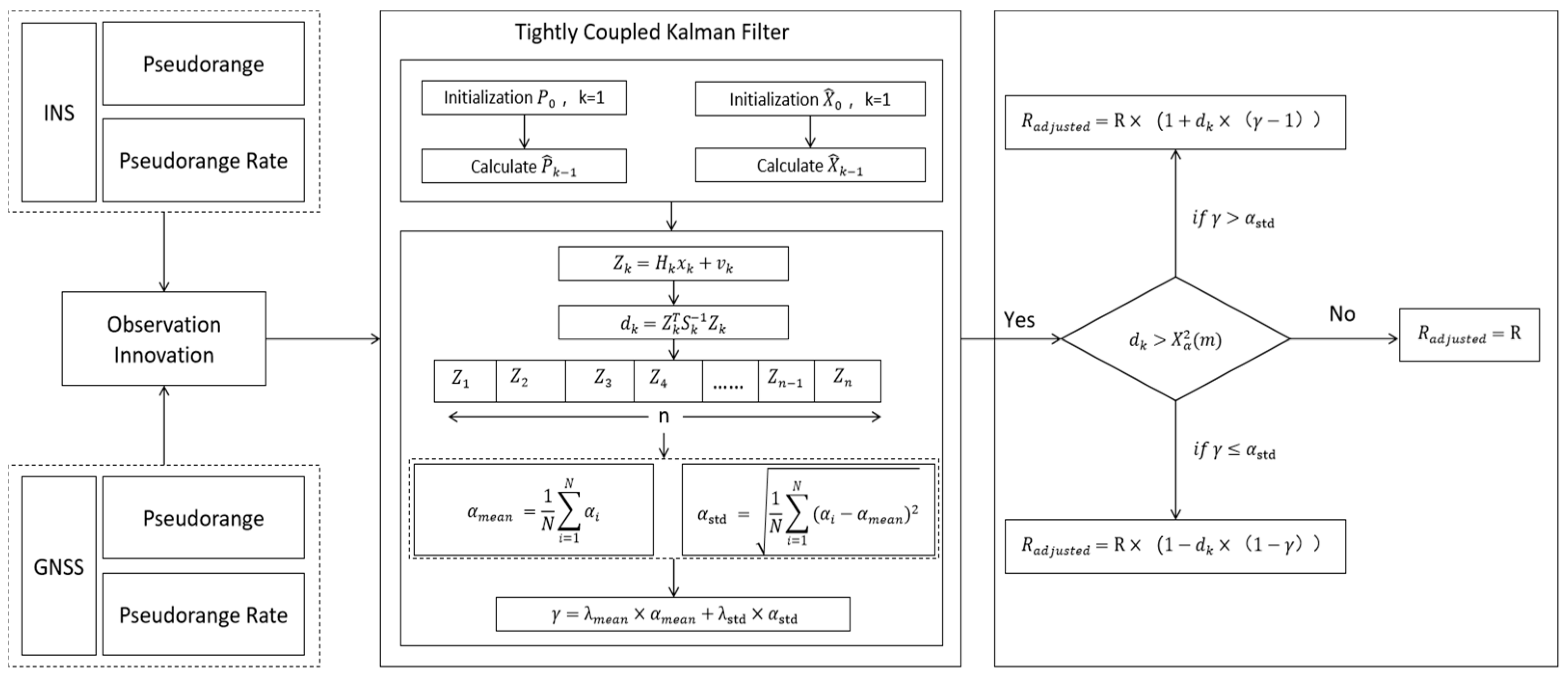
(3) Improved AREKF Based on Sliding Window: The Improved Adaptive Robust Extended Kalman Filter (IAREKF) algorithm based on a sliding window is shown in Figure 3. By introducing a sliding window framework for estimating the observation noise covariance matrix, its adaptability to observation noise in GNSS/INSs is enhanced. In this method, the predicted residuals are first calculated using the theoretical residual covariance, and the magnitude of the residuals is measured using Mahalanobis distance. Subsequently, the historical residuals are updated using a sliding window, and the mean and standard deviation of the residuals are calculated for use in calculating the adaptive factor. The adaptive factor combines the residual mean, residual fluctuation, and threshold ratio to determine whether the magnitude of the observation noise needs to be increased or decreased. The observation noise covariance matrix R is adjusted according to the adaptive factor, thereby improving the robustness and stability of the filter in complex dynamic environments.
The residuals and Mahalanobis distance can be calculated using Equations (24) and (32), and then the sliding window is updated to store the historical residuals.
After introducing the sliding window, the residual mean α mean and residual standard deviation α std are calculated for use in the calculation of the adaptive factor where N represents the sliding window size:
α mean = 1 N i = 1 N α i
α std = 1 N i = 1 N α i α mean 2
The threshold is set by Equation (34) to determine whether the residual is too large.
Subsequently, combination factors λ mean and λ std are introduced to control the impact of residual mean and residual volatility. The adaptive factor γ is calculated based on the combination factors, residual mean, and residual standard deviation.
γ = λ mean × α mean + λ std × α std
Finally, the observation noise covariance matrix R is adjusted based on the residual mean and residual fluctuation, as shown in the following equation:
R adjusted = R × ( 1 + d k × ( γ 1 ) ) i f   γ > α std   R × ( 1 d k × ( 1 γ ) ) i f     γ α std  
The implementation process is presented in Table 1.
This section has introduced the principles and implementation process of the IAREKF algorithm, focusing on the system model and filtering techniques. The next section will provide a detailed description of the experimental setup, including the methods, equipment, and navigation route used in the Arctic environment. This will allow for a comprehensive understanding of how the algorithm is applied and tested in real-world conditions.

3. Results

This section mainly introduces the experiments designed in this paper, the experimental equipment and equipment parameters, specifically including the experimental control group design, experimental data acquisition equipment and sensor parameter specifications.

3.1. Experimental Description

This paper designs experiments to verify the effectiveness of the proposed method. Under normal GNSS availability, the system fuses GNSS observations with INS output for navigation at a frequency of once per second. First, a tightly coupled integrated navigation algorithm is adopted, and an improved adaptive robust extended Kalman filter (IAREKF) algorithm is introduced for filtering to enhance the robustness of the system. To verify the performance of the proposed method, this study compares the results of the combined tightly coupled navigation algorithm and IAREKF method with the following scenarios: a loosely coupled navigation algorithm using only EKF, a tightly coupled navigation algorithm using EKF, and a tightly coupled navigation algorithm using AREKF. These comparisons demonstrate the performance advantages of the combined tightly coupled navigation algorithm and IAREKF method in navigation.
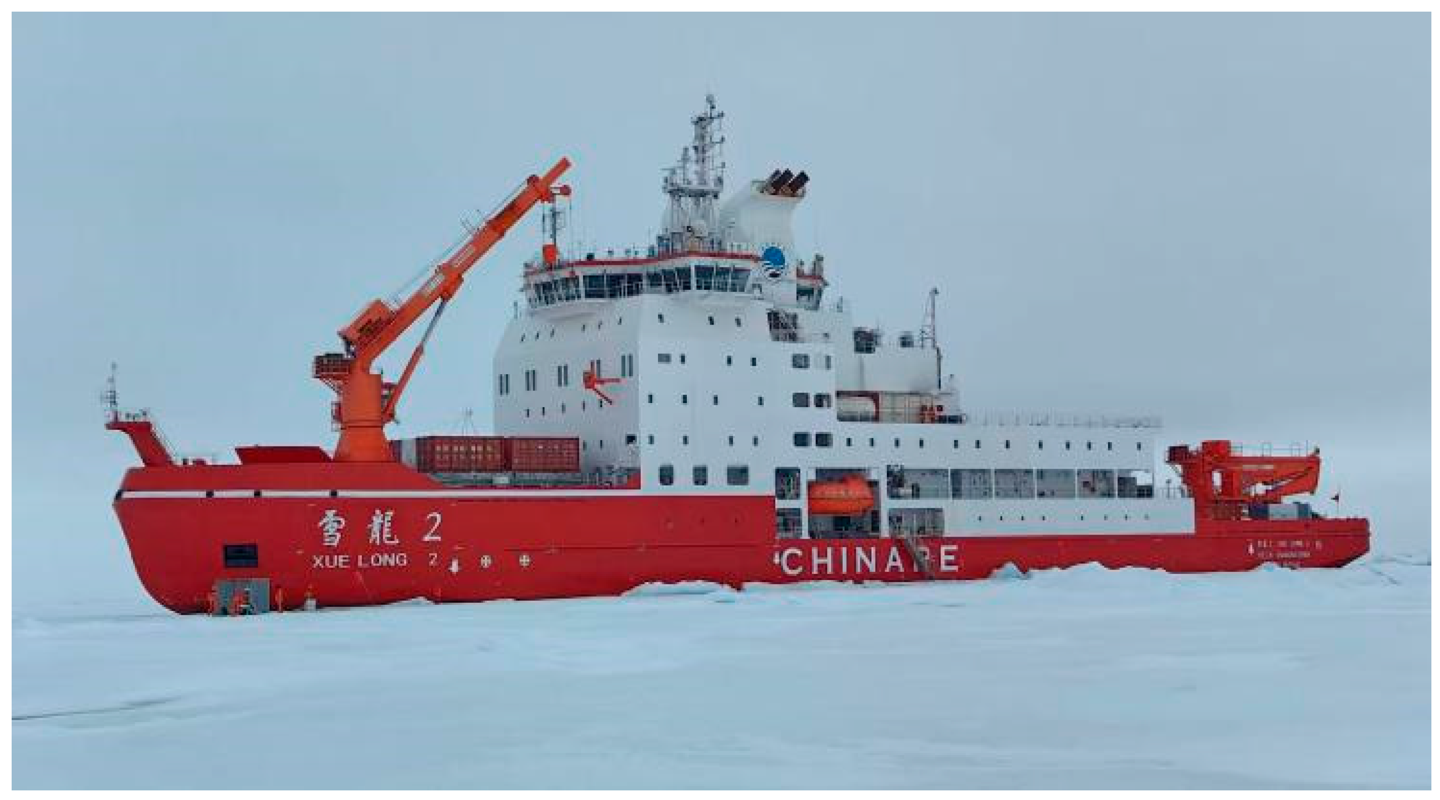
To evaluate the accuracy of the tightly coupled integrated navigation system based on IAREKF under complex navigation conditions in the Arctic Ocean, experimental data were primarily obtained from the Chinese polar research vessel “Xuelong 2” and post-processed for analysis. Operated by the Polar Research Institute of China, the Xuelong 2 is a state-owned icebreaker equipped with an advanced navigation system. As an experimental platform for high-latitude testing, the Xuelong 2 is shown in Figure 4.

3.2. Experimental Equipment

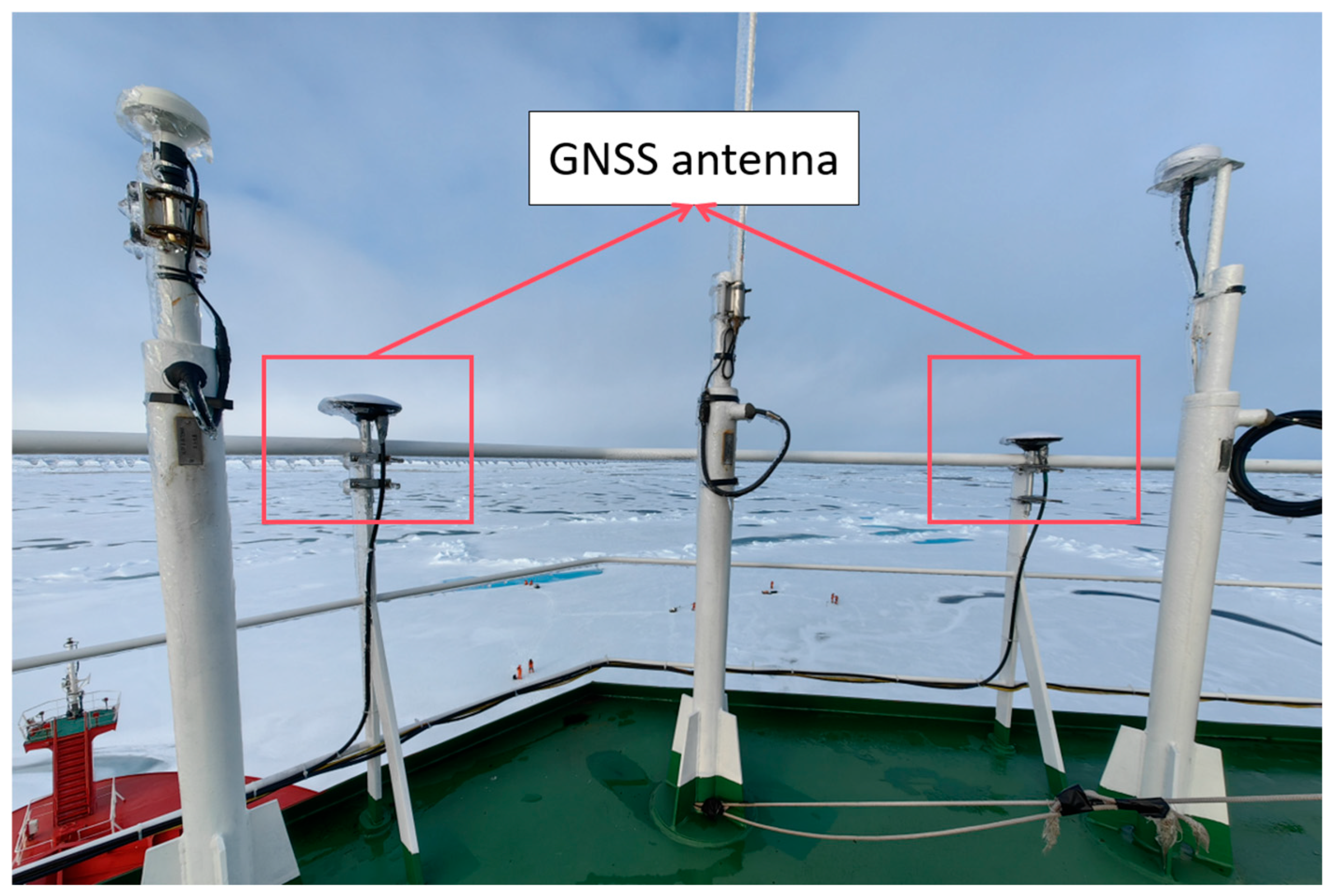
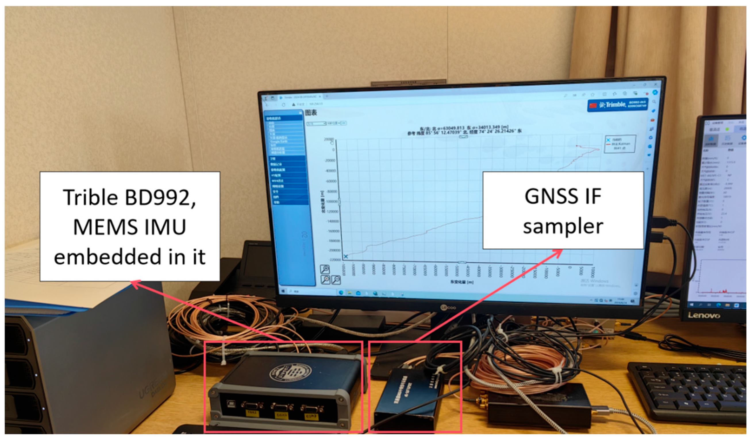
The onboard equipment installation of Xuelong 2, shown in Figure 5 and Figure 6, primarily includes the GNSS antenna, Trimble BD992, MEMS IMU, GNSS intermediate frequency sampler, and other equipment.
The onboard sensor suite included:
(1)
A STIM300 (Sensonor AS, Horten, Norway), a tactical-grade MEMS IMU co-located with a Trimble BD992 dual-frequency GNSS receiver inside a rigid enclosure.
(2)
A GNSS Intermediate Frequency (IF) sampler (HG-SOFTGPS01-B) for capturing raw GNSS signals.
(3)
Two GNSS antennas rigidly mounted on the vessel deck to reduce lever-arm effects.
The Trimble BD992 operated in automatic mode and tracked GPS, BDS, GLONASS, and Galileo signals. All sensors were tightly time-synchronized via Pulse-Per-Second (PPS) signals, and the entire sensor assembly was installed on a vibration-isolated platform to ensure stable operation.
The MEMS IMU provided tri-axis angular velocity and linear acceleration at a sampling rate of 1000 Hz, while the Trimble BD992 receiver operated at a downsampled rate of 1 Hz to match the navigation filter frequency and facilitate data fusion. The IF sampler was also deployed to capture raw multi-constellation GNSS IF data sampled at 16.369 MHz for pre-processing and signal quality assessment. The horizontal positioning accuracy of the BD992 was specified as 0.50 m under nominal conditions. Key specifications of the onboard sensors are summarized in Table 2.

3.3. Experimental Equipment and Route

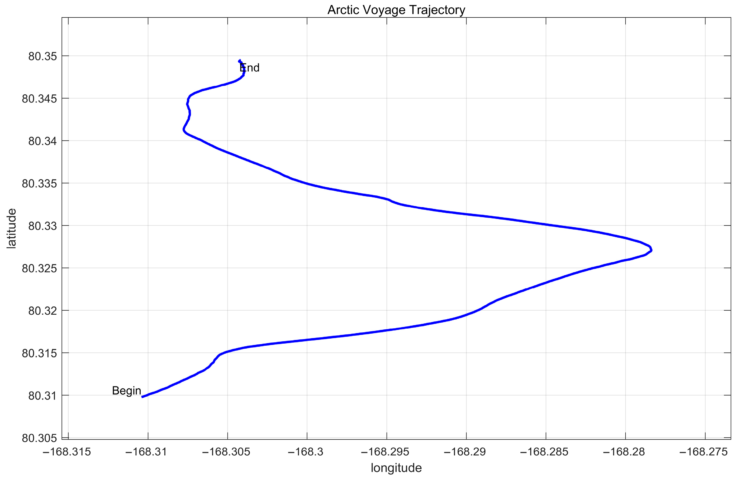
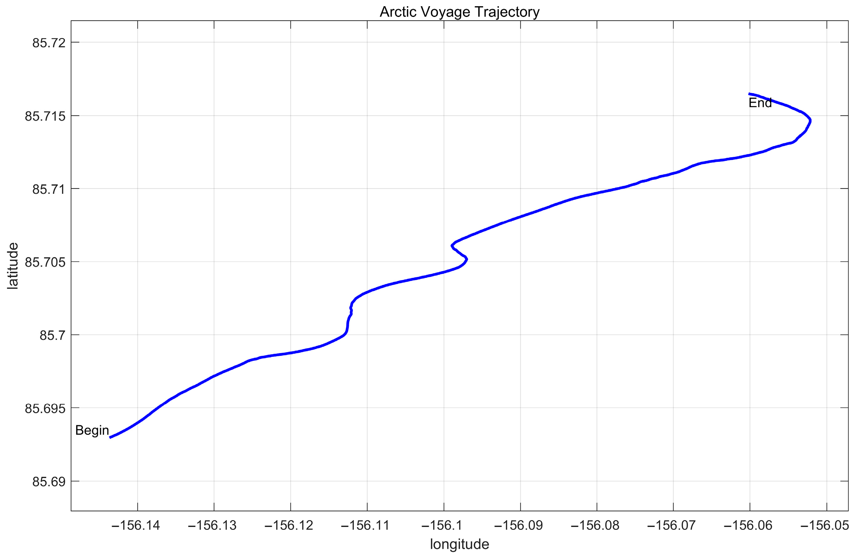
During the experiment, the real-time positioning output of the BD992 GNSS receiver was transmitted via serial port to a laptop and recorded for post-processing. The BD992 receiver provides decimeter-level positioning accuracy under normal conditions. Although inherent errors exist in polar environments due to satellite geometry, ionospheric effects, multipath interference, and receiver noise, the application of a backward smoothing (inverse filtering) technique effectively reduces transient deviations and refines the trajectory. The resulting smoothed trajectory exhibits a positioning accuracy one or more orders of magnitude higher than that of the integrated navigation algorithms evaluated in this study. Therefore, the refined BD992 trajectory can be reasonably regarded as the reference for assessing navigation accuracy. The satellite trajectory plots shown in Figure 7 and Figure 8 show the navigation tracks corresponding to two segments at latitudes of 80.3° and 85.7°, respectively, each segment lasting over 1300 s.
In order to validate the effectiveness of the proposed IAREKF algorithm, Section 4 will present the experimental results. These results will be compared against other navigation techniques, including GNSS/INS loosely coupled integration, the traditional EKF, and the standard AREKF. This comparative analysis will demonstrate the improvements in accuracy and robustness offered by the IAREKF algorithm, particularly under the challenging conditions of the Arctic environment.

4. Discussion

4.1. Arctic GNSS Navigation Features

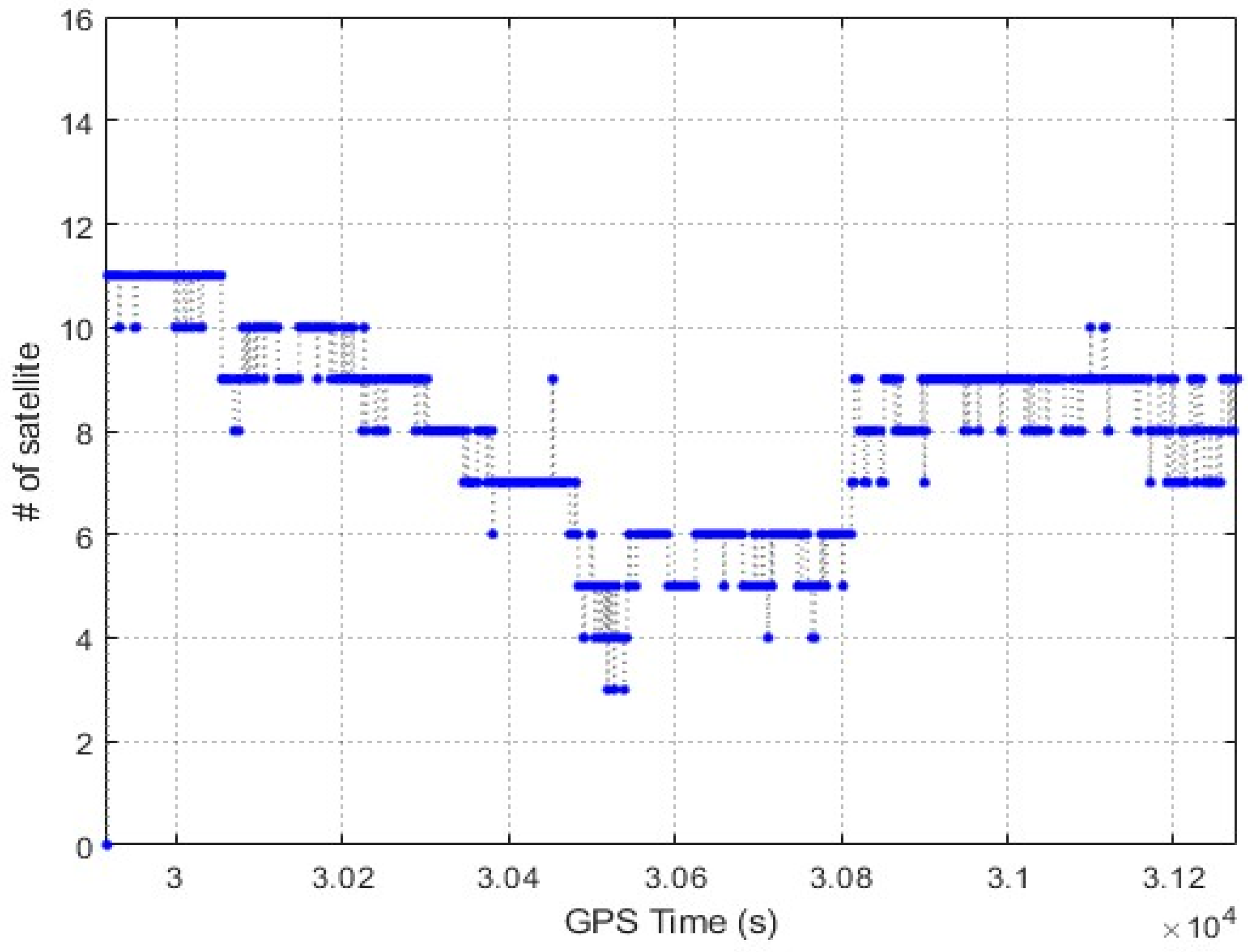
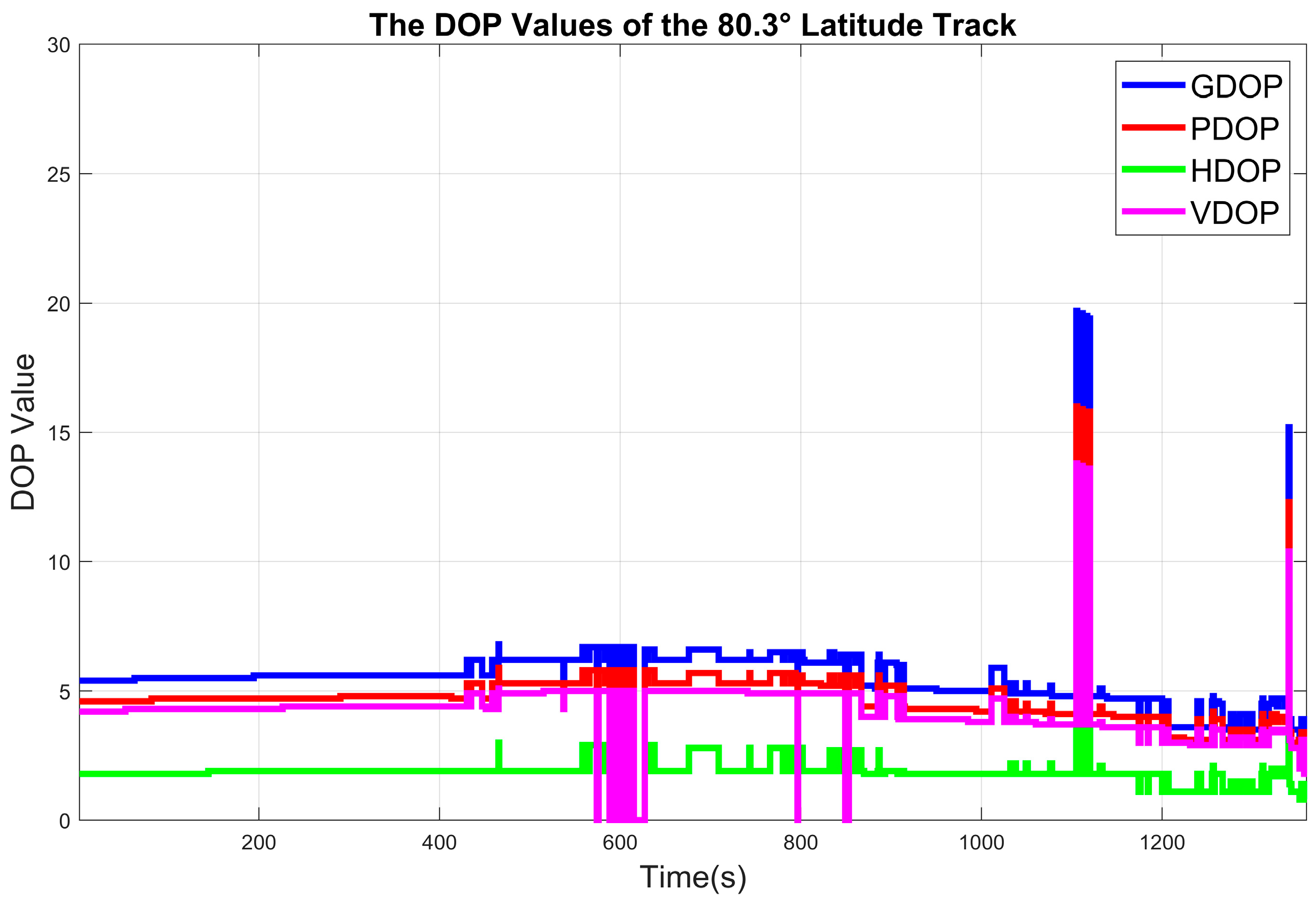
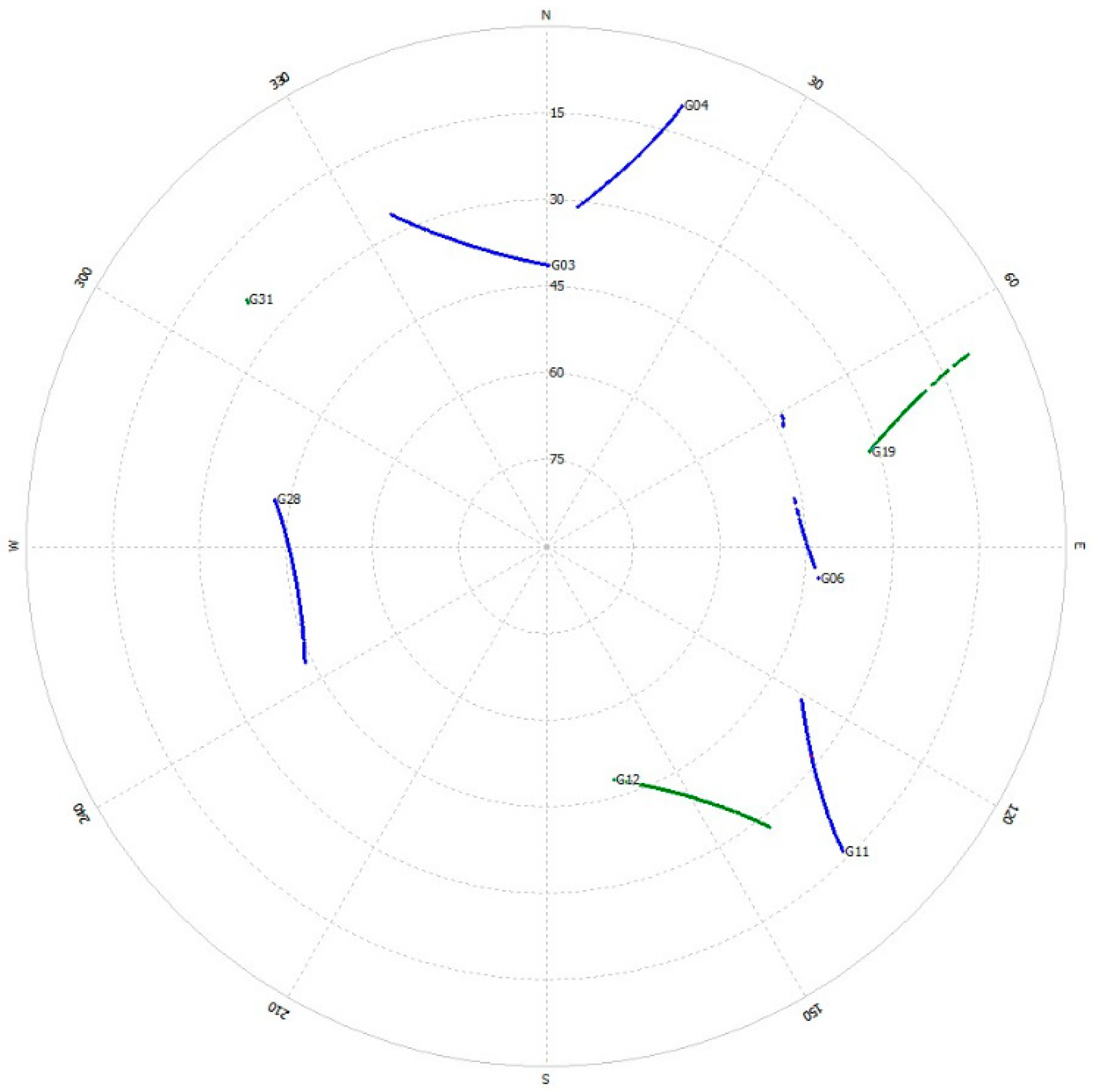
In the Arctic regions with high latitudes, factors such as low satellite elevation angles and poor geometric performance often significantly impact navigation accuracy. These issues are especially prominent in Arctic navigation, as shown in Figure 9, Figure 10 and Figure 11. Figure 9 illustrates the number of satellites during the first segment of the Arctic voyage, while Figure 10 and Figure 11 display the satellite distribution and DOP variations near latitude 80.3°. At latitude 80.3°, the number of satellites is relatively low, and most satellites have elevation angles below 30°, reflecting the typical low-elevation characteristics of Arctic satellites. Furthermore, the peak GDOP (Geometric Dilution of Precision) is approximately 20, indicating relatively poor average geometric performance.
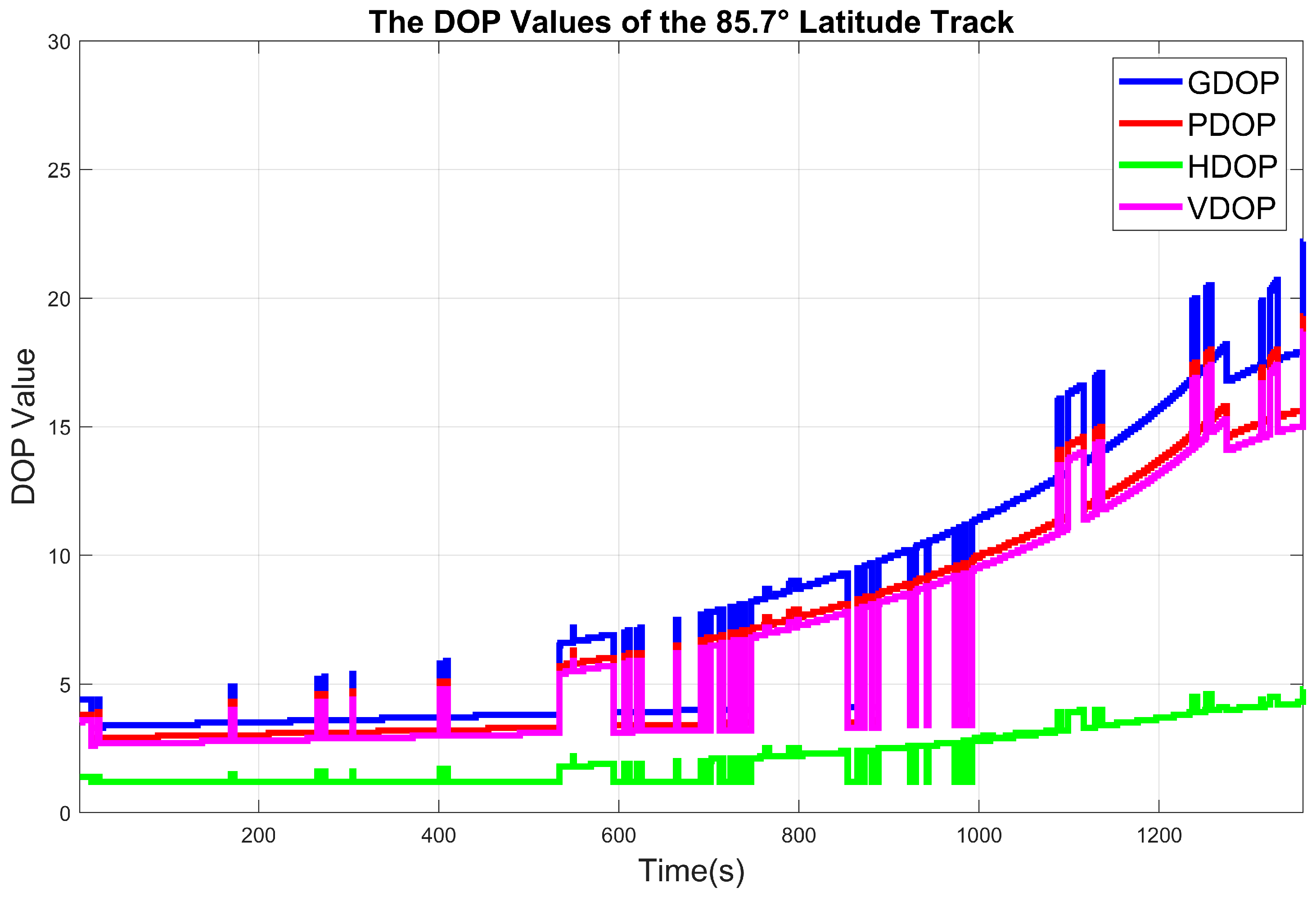
Figure 12 shows the number of satellites during the first phase of the Arctic voyage, while Figure 13 and Figure 14 display the satellite distribution and variations in the Geometric Dilution of Precision (GDOP) near latitude 85.7°. At latitude 85.7°, the number of satellites is relatively low, and some satellites have elevation angles below 30°, reflecting the typical low-elevation characteristics of Arctic satellites. Additionally, the peak GDOP is approximately 22, indicating relatively poor average geometric accuracy.
The differences in the color tracks of the captured satellites in Figure 10 and Figure 13 represent different frequency bands received by the receiver. Blue indicates satellites operating in the L1, L2, and L5 bands. Green indicates satellites operating in the L1 and L2 bands.
In the experiment, the results of the combined tightly coupled navigation algorithm and IAREKF method were compared with the following cases: loosely coupled navigation algorithm using only EKF, tightly coupled navigation algorithm using EKF, and tightly coupled navigation algorithm using AREKF. These comparative experiments validate the improvements brought about by the tightly coupled navigation algorithm and the improved adaptive robust Kalman filter. In the evaluation, the maximum error and root mean square error (RMSE) were selected as the primary performance indicators. East–west and north-north errors were also calculated to evaluate positioning accuracy in the two-dimensional plane. The corresponding formulas are as follows:
RMSE Horizontal = 1 m k = 1 m err k , east 2 + err k , north 2
In Section 4.2 and Section 4.3, Experiments 1 and 2 are used to verify the effectiveness of the proposed method. Experiment 1 uses data collected from the icebreaker “Xuelong 2” along its route at approximately 80.3° latitude. Experiment 2 uses data collected from the same ship along its route at approximately 85.7° latitude. These two experiments aim to evaluate the performance of the proposed algorithm under different Arctic navigation conditions. By comparing the results of the proposed method with those of other algorithms, the effectiveness and robustness of the tightly coupled IAREKF algorithm in terms of positioning accuracy and system stability in the harsh Arctic environment are demonstrated.

4.2. Experimental 1 Results

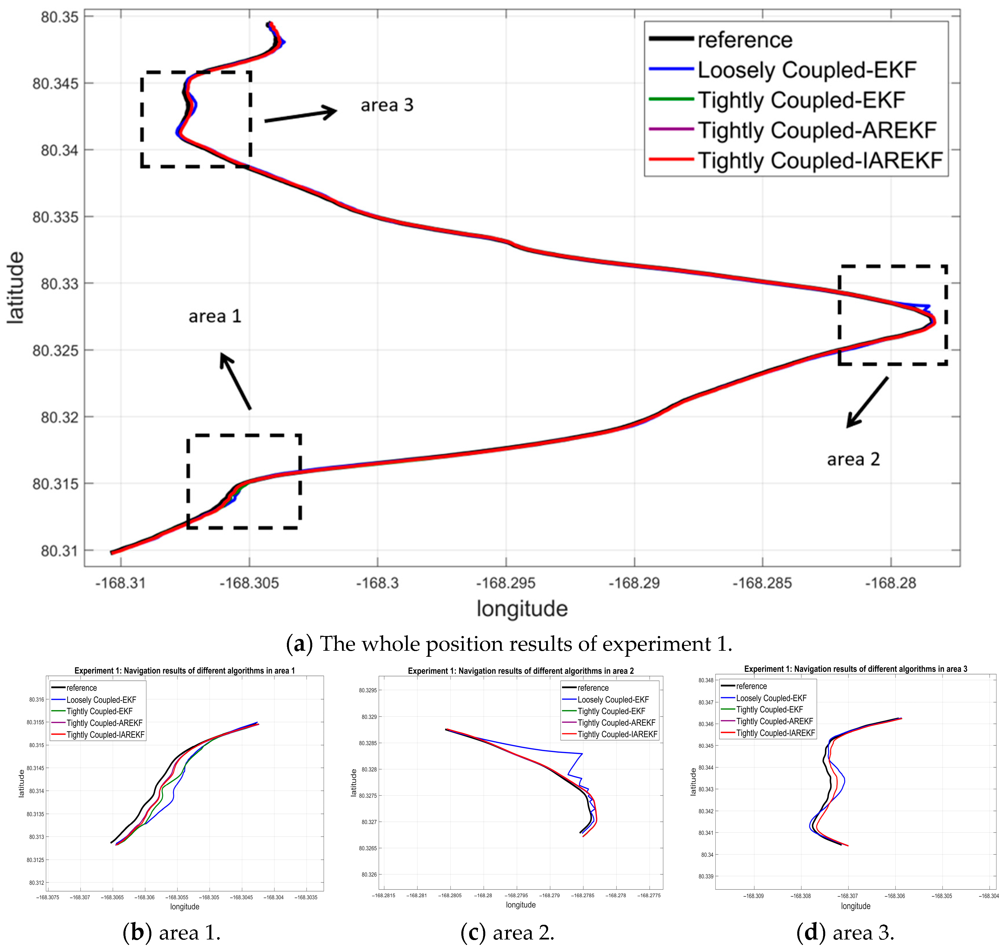
Figure 15 shows the navigation results of different algorithms on a route at latitude 80.3°, where (b), (c), and (d) show the navigation results of different algorithms in three regions. Five control groups were set up in the experiment: reference trajectory (black), loosely coupled EKF (blue), tightly coupled EKF (green), tightly coupled AREKF (purple), and tightly coupled IAREKF (red).
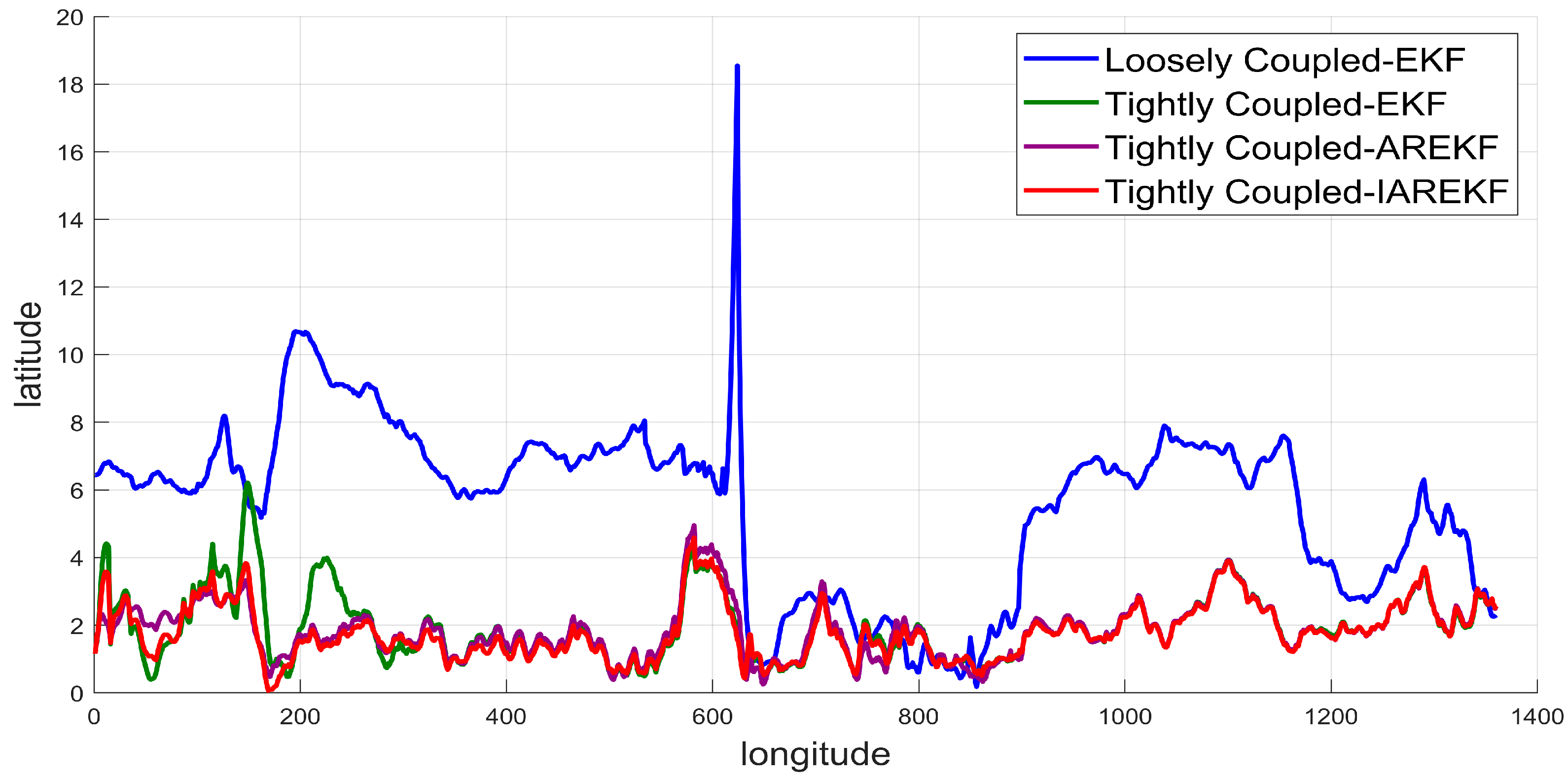
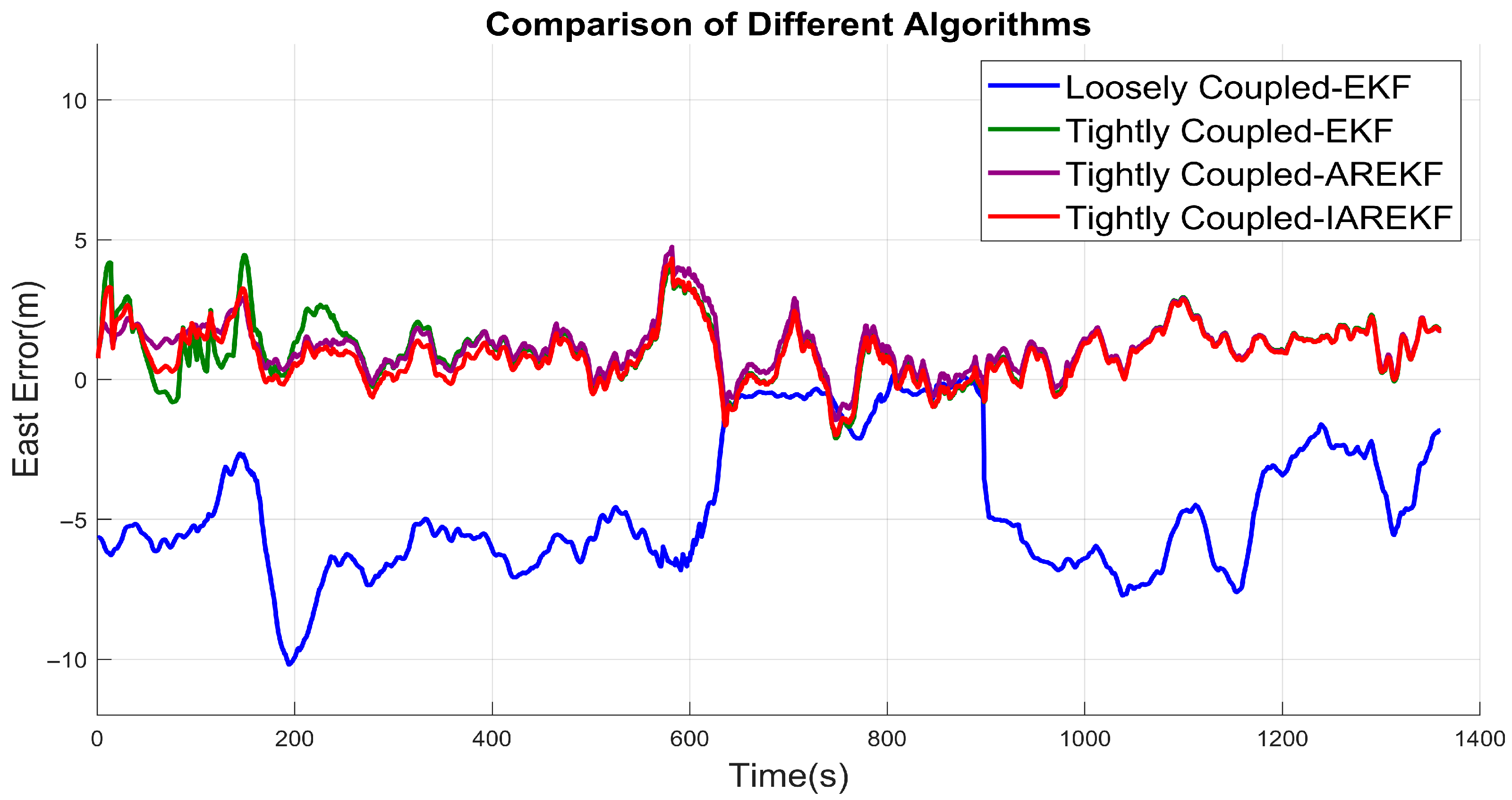
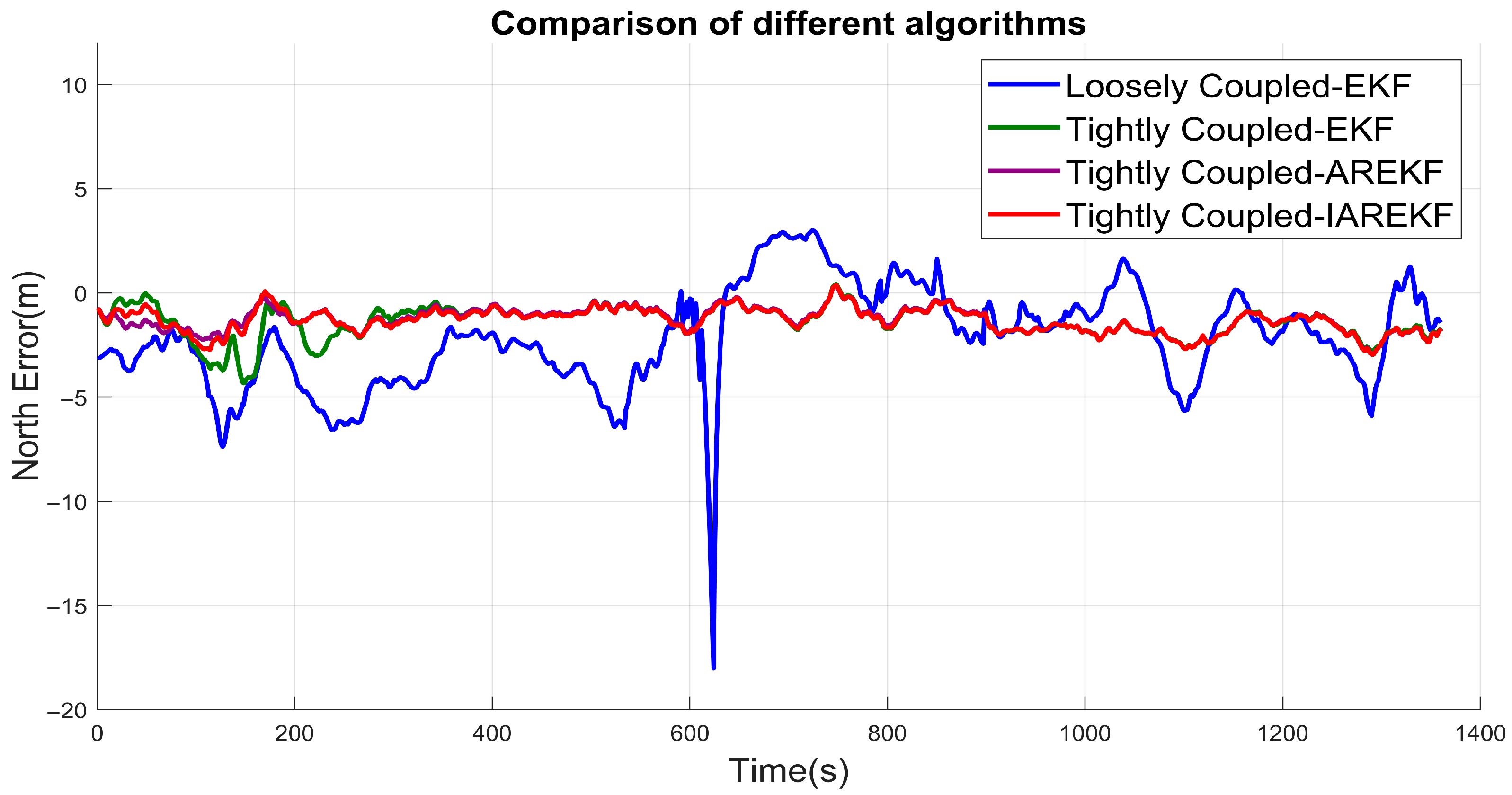
As shown in Figure 16, Figure 17 and Figure 18, the Tightly Coupled-IAREKF navigation algorithm exhibits the best convergence in terms of horizontal positioning error, northward positioning error, and eastward positioning error. This demonstrates that the proposed IAREKF can effectively suppress error propagation and provide a more accurate and reliable navigation solution in the complex and dynamic environment of the Arctic. Table 3 and Table 4 provide a detailed comparison of the positioning errors of different algorithms, highlighting the performance differences among the various methods.
It can be observed that the Tightly Coupled-IAREKF algorithm achieves the highest horizontal positioning accuracy within the 1360-s Arctic route. A comparison of navigation results between Tightly Coupled-EKF and Loosely Coupled-EKF shows a reduction in both maximum error and root mean square error, indicating further improvement in positioning accuracy. Compared to the Tightly Coupled-EKF algorithm, the Tightly Coupled-IAREKF algorithm further improves positioning accuracy. Compared to the traditional Loosely Coupled-EKF algorithm, the Tightly Coupled-IAREKF algorithm reduces the maximum eastward and northward positioning errors by 57.53% and 83.5%, respectively, while reducing the RMSE for eastward, northward, and horizontal positions by 74.07%, 55.27%, and 67.63%, respectively. These results demonstrate that the proposed Tightly Coupled-IAREKF algorithm effectively reduces positioning errors and improves the system’s navigation performance in the complex Arctic environment.

4.3. Experimental 2 Results

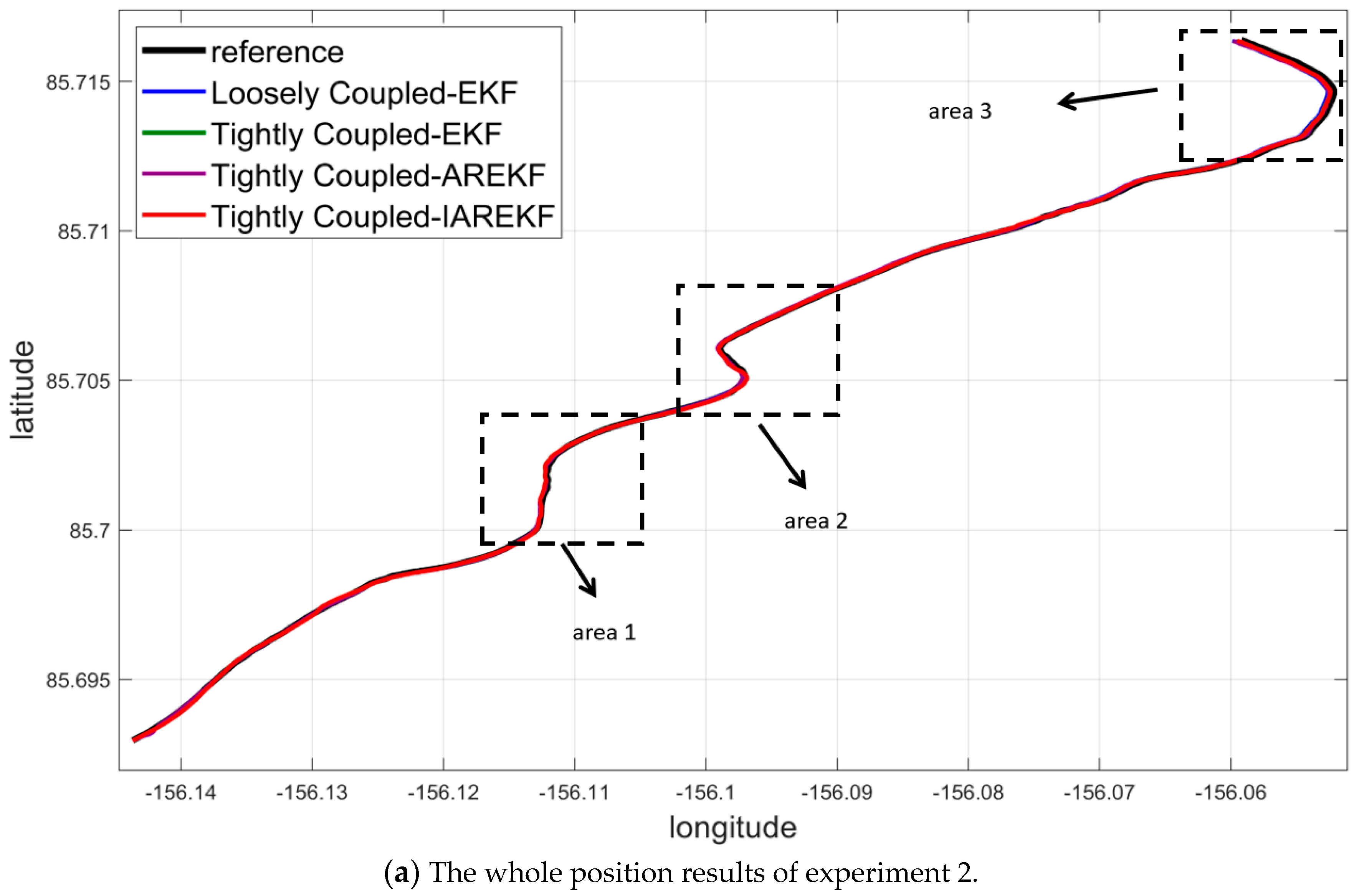
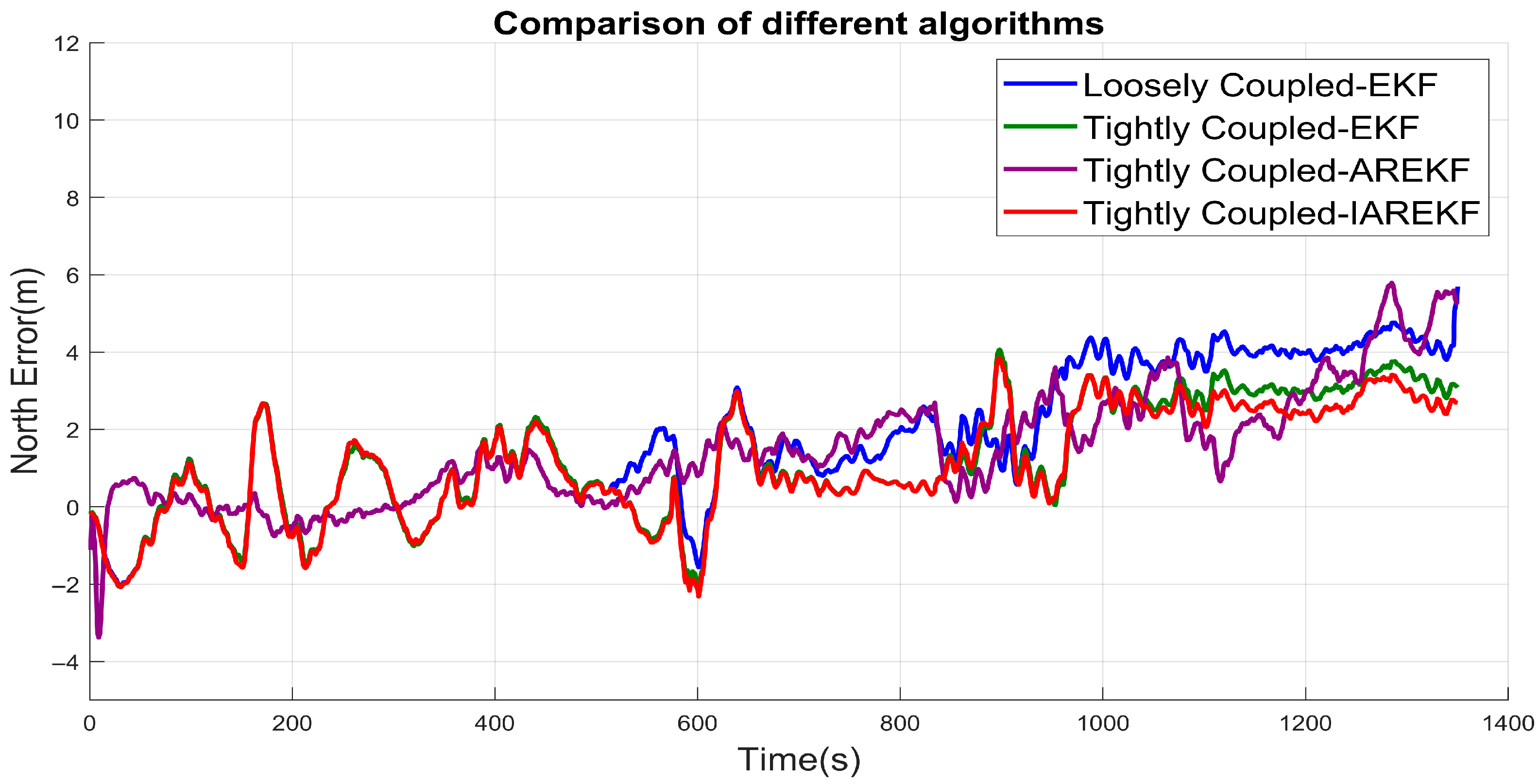
Figure 19 shows the navigation results of different algorithms on a route at latitude 85.7°, where (b), (c), and (d) show the navigation results of different algorithms in three regions. Five control groups were set up in the experiment: reference trajectory (black), Loosely Coupled-EKF (blue), Tightly Coupled-EKF (green), Tightly Coupled-AREKF (purple), and Tightly Coupled-IAREKF (red).
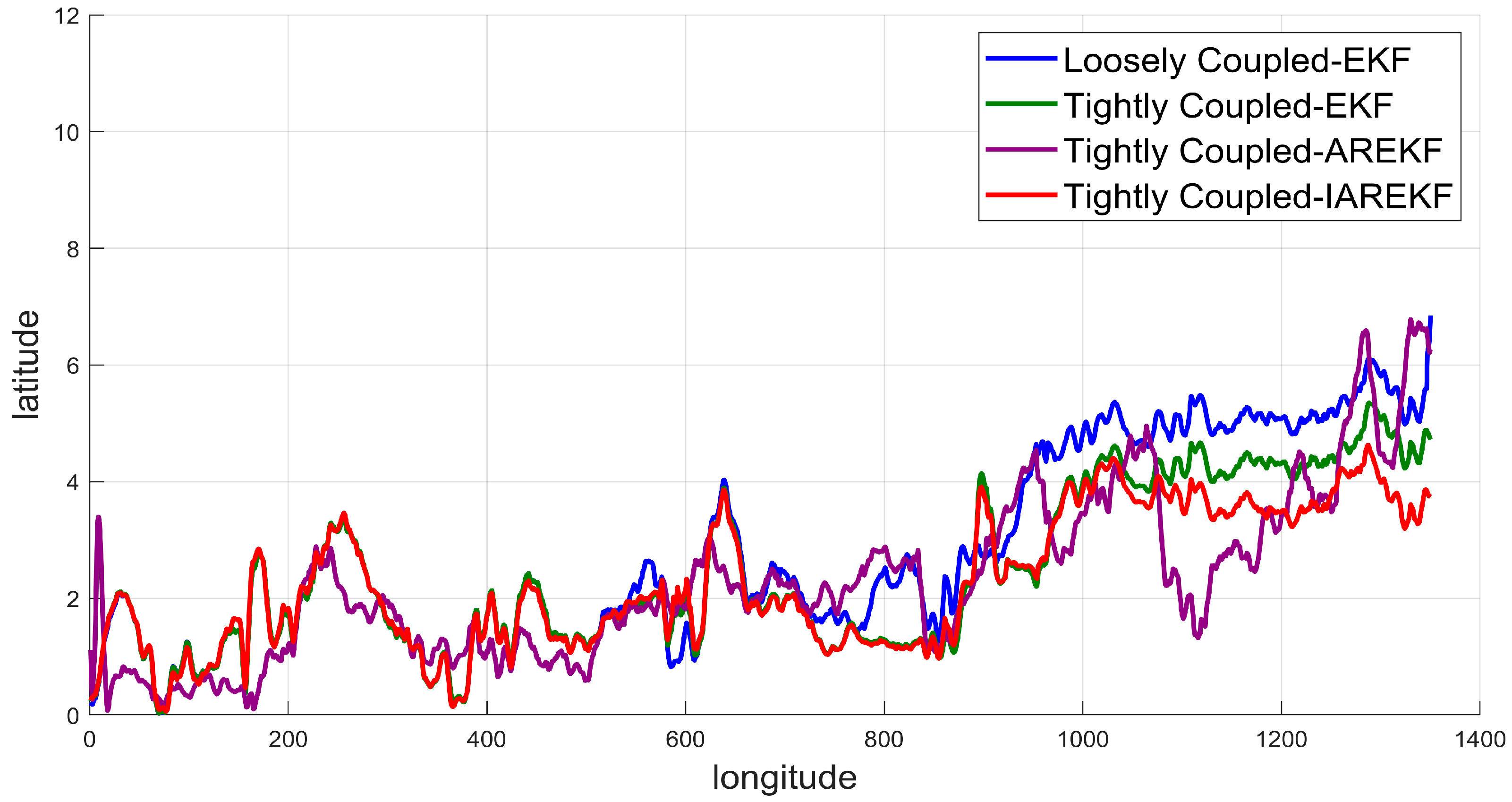
As shown in Figure 20, Figure 21 and Figure 22, the Tightly Coupled-IAREKF navigation algorithm exhibits the best convergence in terms of horizontal positioning error and northward positioning error. This demonstrates that the proposed IAREKF can effectively suppress error propagation and provide a more accurate and reliable navigation solution in the complex and dynamic environment of the Arctic. Table 5 and Table 6 provide a detailed comparison of the positioning errors of different algorithms, highlighting the performance differences among the various methods.
It can be observed that, in the 1350-s Arctic navigation segment, the Tightly coupled-IAREKF algorithm achieved the highest horizontal positioning accuracy. A comparison of the navigation results between the Tightly coupled-EKF algorithm and the Loosely coupled-EKF algorithm shows that the root mean square error (RMSE) for the Tightly coupled-EKF algorithm was reduced, resulting in further improvement in positioning accuracy. Compared to the Tightly coupled-EKF algorithm, the Tightly coupled-IAREKF algorithm further enhanced the positioning accuracy. In comparison with the traditional Loosely coupled-EKF algorithm, the Tightly coupled-IAREKF algorithm reduced the maximum eastward and northward positioning errors by 11.44% and 32.62%, respectively, while the RMSE for eastward, northward, and horizontal positions was reduced by 12.79%, 28.58%, and 21.7%, respectively. These results indicate that the proposed tightly coupled-IAREKF algorithm effectively reduces positioning errors and improves the system’s navigation performance in the challenging Arctic environment.
Overall, the results of Experiments 1 and 2 clearly demonstrate that the tightly coupled IAREKF algorithm has a significant advantage in improving positioning accuracy compared to the tightly coupled and loosely coupled EKF algorithms. The reduction in root mean square errors (RMSEs) in the east, north, and horizontal directions proves that the proposed algorithm effectively mitigates the impact of environmental noise on navigation accuracy in the Arctic environment. These results validate the effectiveness of our proposed method. By introducing the sliding window technique, the tightly coupled IAREKF algorithm can dynamically adjust the observation noise covariance matrix, thereby effectively reducing the impact of non-Gaussian noise and sudden interference on navigation results, and improving the robustness and stability of the shipborne navigation system in complex environments.

5. Conclusions

To address the challenges of robust shipboard navigation systems in the complex Arctic environment, this study proposes an improved adaptive robust extended Kalman filter (IAREKF) method based on tightly coupled GNSS/INS. First, the IAREKF is used to calculate residuals and Mahalanobis distances, and the anomalies of observations are assessed using a chi-square test, thereby dynamically adjusting the observation noise covariance matrix to enhance the filter’s anti-interference capability in the complex Arctic environment. However, the state estimation accuracy of AREKF is still affected by GNSS signal degradation, leading to a decrease in navigation and positioning accuracy. To further improve the filter’s robustness and positioning accuracy, a sliding window mechanism is introduced, dynamically adjusting the observation noise covariance matrix using historical residual information, effectively enhancing the system’s stability in harsh environments. Experimental results using real navigation data show that the proposed method significantly improves horizontal positioning accuracy compared to the Loosely coupled-EKF, increasing it by 61.78% and 21.7%, respectively. The overall positioning error remains at the meter level, providing stable and reliable navigation results.
These results demonstrate that the proposed Improved Adaptive Robust Extended Kalman Filter (IAREKF) method exhibits excellent performance in the mid-to-high latitudes of the Arctic, effectively addressing navigation challenges in complex environments. However, despite its superior performance and effectiveness in complex environments, the proposed IAREKF method still has some limitations. One limitation is the impact of extreme GNSS signal attenuation, which still affects the accuracy of state estimation. Furthermore, the algorithm’s performance may vary in the Arctic region with its diverse terrain and environmental conditions. Further research is needed to address these challenges, such as enhancing the algorithm’s adaptability to more severe GNSS signal outages or integrating complementary sensors to further improve robustness.
Future work will explore the real-time deployment of the IAREKF algorithm on autonomous platforms such as UAVs and autonomous vehicles to evaluate its feasibility and performance in practical applications. In addition, applying machine learning techniques to adaptive noise filtering and dynamic system tuning can further improve the robustness and accuracy of navigation systems.

Author Contributions

Conceptualization, W.L.; Methodology, Y.H.; Software, T.Q.; Validation, S.F.; Writing—original draft, T.Q.; Data curation, T.-H.H.; Review and Editing, S.W.; Supervision, B.H. All authors have read and agreed to the published version of the manuscript.

Funding

This research received no external funding.

Data Availability Statement

Due to the relative difficulty in obtaining this dataset and its continued use in subsequent research, it cannot be made public.

Acknowledgments

We sincerely thank all the teachers and students for their valuable support in the relevant analysis work of this study.

Conflicts of Interest

The authors declare no conflicts of interest.

Abbreviations

The following abbreviations are used in this manuscript:
AUVautonomous underwater vehicle
GNSSsGlobal Navigation Satellite Systems
INSsInertial Navigation Systems
IAREKFImproved Adaptive Robust Extended Kalman Filter
AREKFAdaptive Robust 27 Extended Kalman Filter
GDOPgeometric dilution of precision
IMUsinertial measurement units
KFKalman filter
MMSEminimum mean square error
EKFExtended Kalman Filter
UKFunscented Kalman filter
CKFcubature Kalman filter
PFparticle filter
AKFAdaptive Kalman Filter
RKFRobust Kalman Filter
ARKFadaptive robust Kalman filter
I-MORKFimproved multiple-outlier-robust Kalman filter
IFIntermediate Frequency
PPSPulse-Per-Second
RMSEroot mean square error

References

  1. Huntington, H.P.; Olsen, J.; Zdor, E.; Zagorskiy, A.; Shin, H.C.; Romanenko, O.; Kaltenborn, B.; Dawson, J.; Davies, J.; Abou-Abbsi, E. Effects of Arctic commercial shipping on environments and communities: Context, governance, priorities. Transp. Res. Part D 2023, 118, 103731. [Google Scholar]
  2. Mahmoud, M.R.; Roushdi, M.; Aboelkhear, M. Potential benefits of climate change on navigation in the northern sea route by 2050. Sci. Rep. 2024, 14, 2771. [Google Scholar] [CrossRef]
  3. Qi, X.; Li, Z.; Zhao, C.; Zhang, Q.; Zhou, Y. Environmental impacts of Arctic shipping activities: A review. Ocean Coast. Manag. 2024, 247, 106936. [Google Scholar] [CrossRef]
  4. Min, C.; Zhou, X.; Luo, H.; Yang, Y.; Wang, Y.; Zhang, J.; Yang, Q. Toward quantifying the increasing accessibility of the Arctic Northeast Passage in the past four decades. Adv. Atmos. Sci. 2023, 40, 2378–2390. [Google Scholar] [CrossRef]
  5. Van der Meeren, C.; Oksavik, K.; Lorentzen, D.A.; Rietveld, M.T.; Clausen, L.B.N. Severe and localized GNSS scintillation at the poleward edge of the nightside auroral oval during intense substorm aurora. J. Geophys. Res. Space Phys. 2015, 120, 10607–10621. [Google Scholar] [CrossRef]
  6. Thayyil, J.P.; McCaffrey, A.M.; Wang, Y.; Themens, D.R.; Watson, C.; Reid, B.; Zhang, Q.; Xing, Z. Global positioning system (GPS) scintillation associated with a polar cap patch. Remote Sens. 2021, 13, 1915. [Google Scholar]
  7. Ben, Y.; Cui, W.; Li, Q. An improved damping method for grid inertial navigation system in polar region. IEEE Trans. Instrum. Meas. 2022, 71, 8505713. [Google Scholar] [CrossRef]
  8. Lu, J.; Shang, J.; Wu, J.; Wang, Y.; Ma, D. Panoramic sea-ice map construction for polar navigation based on multi-perspective images projection and camera poses rectification. IEEE Trans. Intell. Transp. Syst. 2025, 26, 3417–3430. [Google Scholar] [CrossRef]
  9. Xu, B.; Hu, J.; Guo, Y. Global integrated navigation position correction algorithm and virtual polar region technology based on normal vector. Measurement 2025, 242, 116031. [Google Scholar] [CrossRef]
  10. Li, Q.; Ben, Y.; Yu, F.; Tan, J. Transversal strapdown INS based on reference ellipsoid for vehicle in the polar region. IEEE Trans. Veh. Technol. 2015, 65, 7791–7795. [Google Scholar] [CrossRef]
  11. Li, Z.; Li, B.; Zhang, X.; Ding, Y.; Xu, T.; Wang, A.; Fan, W. Polar Integrated Navigation Algorithm Based on Transverse Earth Coordinate System. In Proceedings of the 2023 38th Youth Academic Annual Conference of Chinese Association of Automation (YAC), Hefei, China, 27–29 August 2023; pp. 363–369. [Google Scholar]
  12. Yastrebova, A.; Höyhtyä, M.; Boumard, S.; Lohan, E.S.; Ometov, A. Positioning in the Arctic region: State-of-the-art and future perspectives. IEEE Access 2021, 9, 53964–53978. [Google Scholar] [CrossRef]
  13. Reid, T.; Walter, T.; Blanch, J.; Enge, P. GNSS Integrity in the Arctic. NAVIGATION J. Inst. Navig. 2016, 63, 469–492. [Google Scholar] [CrossRef]
  14. de Jong, K.; Goode, M.; Liu, X.; Stone, M. Precise GNSS positioning in Arctic regions. In Proceedings of the OTC Arctic Technology Conference, Houston, TX, USA, 10–12 February 2014. [Google Scholar]
  15. Niu, X.; Dai, Y.; Liu, T.; Chen, Q.; Zhang, Q. Feature-based GNSS positioning error consistency optimization for GNSS/INS integrated system. GPS Solut. 2023, 27, 89. [Google Scholar] [CrossRef]
  16. Gao, W.; Zhan, X.; Yang, R. INS-aiding information error modeling in GNSS/INS ultra-tight integration. GPS Solut. 2024, 28, 35. [Google Scholar] [CrossRef]
  17. Wang, Y.; Wang, Q.; Zhang, H.; Duan, X. A Low-Cost GNSS/INS integration method aided by Cascade-LSTM Pseudo-Velocity measurement for bridging GNSS outages. Measurement 2025, 240, 115518. [Google Scholar] [CrossRef]
  18. Shen, Z.; Li, X.; Wang, X.; Wu, Z.; Li, X.; Zhou, Y.; Li, S. A novel factor graph framework for tightly coupled GNSS/INS integration with carrier-phase ambiguity resolution. IEEE Trans. Intell. Transp. Syst. 2024, 25, 13091–13105. [Google Scholar] [CrossRef]
  19. Falco, G.; Pini, M.; Marucco, G. Loose and tight GNSS/INS integrations: Comparison of performance assessed in real urban scenarios. Sensors 2017, 17, 255. [Google Scholar] [CrossRef]
  20. Broumandan, A.; Lachapelle, G. Spoofing detection using GNSS/INS/odometer coupling for vehicular navigation. Sensors 2018, 18, 1305. [Google Scholar] [CrossRef] [PubMed]
  21. Dixon, R.; Bobye, M.; Kruger, B.; Jacox, J. GNSS/INS sensor fusion with on-board vehicle sensors. In Proceedings of the 33rd International Technical Meeting of the Satellite Division of The Institute of Navigation (ION GNSS+ 2020), Online, 21–25 September 2020; pp. 424–446. [Google Scholar]
  22. Ma, C.; Pan, S.; Gao, W.; Wang, H.; Liu, L. Variational Bayesian-based robust adaptive filtering for GNSS/INS tightly coupled positioning in urban environments. Measurement 2023, 223, 113668. [Google Scholar] [CrossRef]
  23. Meng, X.; Tan, H.; Yan, P.; Zheng, Q.; Chen, G.; Jiang, J. A GNSS/INS integrated navigation compensation method based on CNN–GRU+ IRAKF hybrid model during GNSS outages. IEEE Trans. Instrum. Meas. 2024, 73, 1–15. [Google Scholar] [CrossRef]
  24. Hargrave, P. A tutorial introduction to kalman filtering. In Proceedings of the IEE Colloquium on Kalman Filters: Introduction, Applications and Future Developments, London, UK, 21 February 1989; pp. 1/1–1/6. [Google Scholar]
  25. Durbin, J.; Koopman, S.J. Time Series Analysis by State Space Methods; Oxford University Press: Oxford, UK, 2012. [Google Scholar]
  26. Liu, W.; Huang, H.; Hu, Y.; Han, B.; Wang, S. A robust GNSS sensors in presence of signal blockage for USV application. Meas. Sci. Technol. 2023, 35, 035124. [Google Scholar] [CrossRef]
  27. Chen, S.; Gao, Y. Improvement of carrier phase tracking in high dynamics conditions using an adaptive joint vector tracking architecture. GPS Solut. 2019, 23, 15. [Google Scholar] [CrossRef]
  28. Ruan, L.; Li, G.; Dai, W.; Tian, S.; Fan, G.; Wang, J.; Dai, X. Cooperative relative localization for UAV swarm in GNSS-denied environment: A coalition formation game approach. IEEE Internet Things J. 2021, 9, 11560–11577. [Google Scholar] [CrossRef]
  29. Li, J.; Yang, G.; Cai, Q. Autonomous aerial–ground cooperative navigation based on information-seeking in GNSS-denied environments. IEEE Internet Things J. 2023, 10, 17058–17069. [Google Scholar] [CrossRef]
  30. Sun, D.; Shen, G.; Li, X.; Zhu, Z.; Chen, P.; Wang, Q.-G. Angle residual weighted adaptive Kalman filtering for mine-used underground monorail crane localization based on UWB/INS integration. IEEE Trans. Instrum. Meas. 2024, 74, 1000711. [Google Scholar] [CrossRef]
  31. Yang, Y.; Wang, X.; Zhang, N.; Gao, Z.; Li, Y. Artificial neural network based on strong track and square root UKF for INS/GNSS intelligence integrated system during GPS outage. Sci. Rep. 2024, 14, 13905. [Google Scholar] [CrossRef]
  32. Song, C.; Huang, Z.; Wu, Y.; Li, S.; Chen, Q. An Innovation-Based Adaptive Cubature Kalman Filtering for GPS/SINS Integrated Navigation. IEEE Sens. J. 2024, 25, 845–857. [Google Scholar] [CrossRef]
  33. Jiang, Y.; Zhu, N.; Renaudin, V. A voting-based robust estimator aided by INS redundancy for tightly coupled GNSS/INS integration in urban environment. IEEE Trans. Veh. Technol. 2025, 74, 13430–13445. [Google Scholar] [CrossRef]
  34. Kalman, R.E.; Bucy, R.S. New results in linear filtering and prediction theory. J. Basic Eng. 1961, 83, 95–108. [Google Scholar] [CrossRef]
  35. Zhao, D.; Qian, H.; Shen, F. Application of neural network and improved unscented kalman filter for GPS/SINS integrated navigation system. In Proceedings of the 2020 IEEE/ION Position, Location and Navigation Symposium (PLANS), Portland, OR, USA, 20–23 April 2020; pp. 177–185. [Google Scholar]
  36. Zhang, S.; Chen, X. Motion constraint aided integrated navigation method based on SVD-CKF. J. Electron. Meas. Instrum. 2022, 36, 82–89. [Google Scholar]
  37. Zhao, S.; Zhou, Y.; Huang, T. A novel method for ai-assisted INS/GNSS navigation system based on CNN-GRU and CKF during GNSS outage. Remote Sens. 2022, 14, 4494. [Google Scholar] [CrossRef]
  38. Fan, G.; Sheng, C.; Yu, B.; Huang, L.; Rong, Q. An indoor and outdoor multi-source elastic fusion navigation and positioning algorithm based on particle filters. Future Internet 2022, 14, 169. [Google Scholar] [CrossRef]
  39. Kruse, T.; Griebel, T.; Graichen, K. Adaptive kalman filtering: Measurement and process noise covariance estimation using kalman smoothing. IEEE Access 2025, 13, 11863–11875. [Google Scholar] [CrossRef]
  40. Shen, K.; Li, Y.; Liu, T.; Zuo, J.; Yang, Z. Adaptive-robust fusion strategy for autonomous navigation in GNSS-challenged environments. IEEE Internet Things J. 2023, 11, 6817–6832. [Google Scholar] [CrossRef]
  41. Uhm, T.; Kim, S. State-of-charge estimation for remaining flying time prediction of small UAV using adaptive robust extended kalman filter. IEEE Trans. Aerosp. Electron. Syst. 2024, 61, 959–977. [Google Scholar]
  42. Ma, C.; Pan, S.; Gao, W.; Liu, L. An improved multiple-outlier-robust kalman filter for GNSS/INS tightly coupled positioning in urban canyons. IEEE Internet Things J. 2025, 12, 48131–48145. [Google Scholar] [CrossRef]
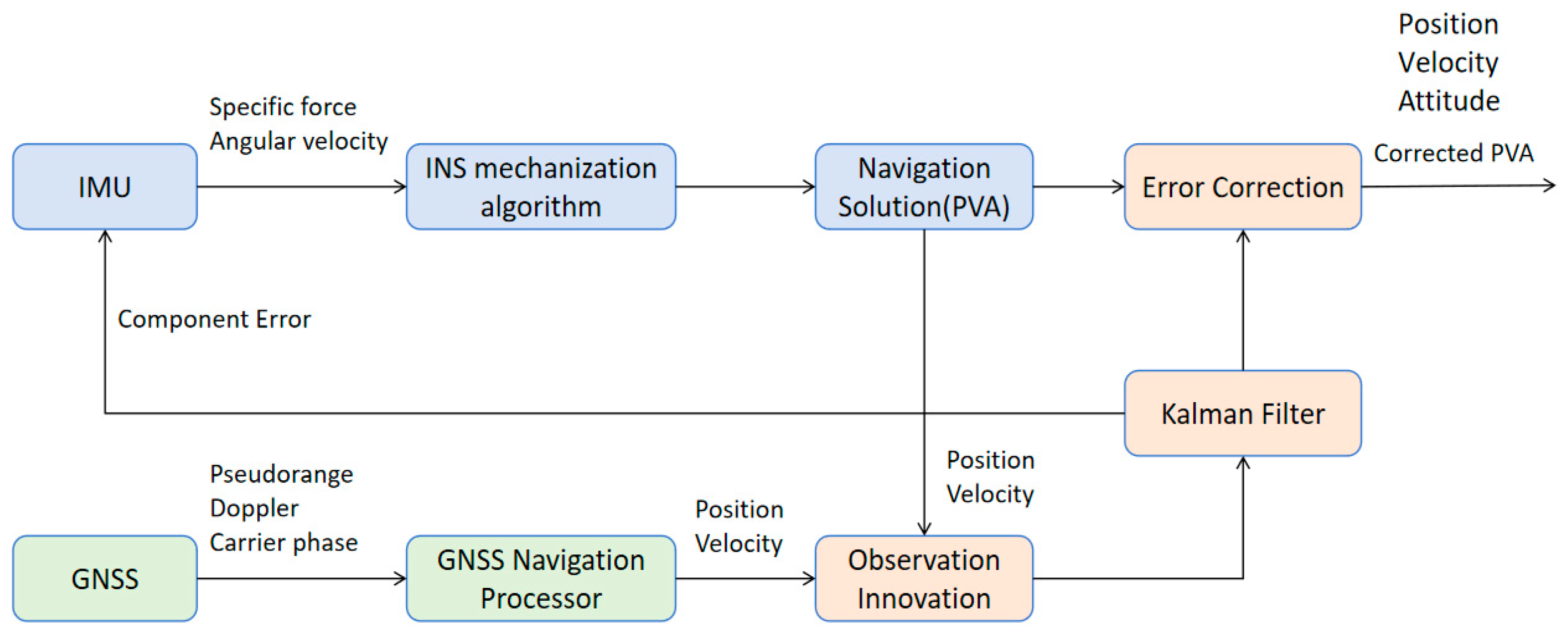
Figure 1. GNSS/INS tightly coupled integrated navigation architecture.
Jmse 13 02395 g001
Figure 2. Framework of Mahalanobis distance-based adaptive robust extended Kalman filter algorithm.
Jmse 13 02395 g002
Figure 3. Framework of improved adaptive robust extended Kalman filter algorithm based on sliding window.
Jmse 13 02395 g003
Figure 4. Xuelong 2 Arctic voyage.
Jmse 13 02395 g004
Figure 5. GNSS antenna.
Jmse 13 02395 g005
Figure 6. Trimble BD992, MEMS IMU, GNSS IF sampler.
Jmse 13 02395 g006
Figure 7. Xuelong 2 Arctic voyage trajectory at latitude 80.3°.
Jmse 13 02395 g007
Figure 8. Xuelong 2 Arctic voyage trajectory at latitude 85.7°.
Jmse 13 02395 g008
Figure 9. Satellite capture count of Xuelong 2 voyage trajectory at latitude 80.3°.
Jmse 13 02395 g009
Figure 10. Satellite sky image at latitude 80.3°.
Jmse 13 02395 g010
Figure 11. DOP value count of Xuelong 2’s trajectory at latitude 80.3°.
Jmse 13 02395 g011
Figure 12. Satellite capture count of Xuelong 2 voyage trajectory at latitude 85.7°.
Jmse 13 02395 g012
Figure 13. Satellite sky image at latitude 85.7°.
Jmse 13 02395 g013
Figure 14. DOP value count of Xuelong 2’s trajectory at latitude 85.7°.
Jmse 13 02395 g014
Figure 15. Experiment 1: Navigation results of different algorithms on a route at latitude 80.3°.
Jmse 13 02395 g015
Figure 16. Horizontal positioning errors of different algorithms during the 1360-s Arctic.
Jmse 13 02395 g016
Figure 17. Experiment 1: Eastward positioning errors of different algorithms during the 1360-s Arctic.
Jmse 13 02395 g017
Figure 18. Experiment 1: Northward positioning errors of different algorithms during the 1360-s Arctic.
Jmse 13 02395 g018
Figure 19. Experiment 2: Navigation results of different algorithms on a route at latitude 85.7°.
Jmse 13 02395 g019aJmse 13 02395 g019b
Figure 20. Horizontal positioning errors of different algorithms during the 1350-s Arctic.
Jmse 13 02395 g020
Figure 21. Experiment 2: Eastward positioning errors of different algorithms during the 1350-s Arctic.
Jmse 13 02395 g021
Figure 22. Experiment 2: Northward positioning errors of different algorithms during the 1350-s Arctic.
Jmse 13 02395 g022
Table 1. Framework for estimating observation noise covariance matrix based on IAREKF.
Input:Observation vector Z k , observation matrix H , observation noise covariance R
Output: R adjusted
Step 1:Initialize sliding window size
Step 2:Calculate the innovation residual covariance matrix S k (27).
Step 3:Calculate the residual vector and calculate the Mahalanobis distance based on the residual, then update the sliding window storing the historical residuals (32).
Step 4:Calculate the residual mean αmean and standard deviation αstd for the calculation of the adaptive factor (38), (39).
Step 5:Set a threshold to determine if the residual is too large (34).
Step 6:Calculate the adaptive factor and adjust the observation noise matrix R based on the mean and fluctuation of the residuals (40).
Step 7:Update the observation noise covariance matrix R based on the adaptive factor. If the residual is too large or the fluctuation is too high, increase the noise (41).
Step 8:Output the updated R adjusted .
Table 2. Specifications of navigation sensors used in Arctic field test.
SensorSpecificationValueUnit
MEMS IMU (STIM 300, Sensonor AS, Norway)Gyro bias instability0.5°/h
Angular random walk0.15 ° / h
Accelerometer bias0.05Mg
Velocity random walk0.07m/s/ h
Sampling rate1000Hz
Trimble
BD992
Sampling rate1Hz
Horizontal accuracy0.50m
IF signal collectorOperating frequency16.369MHz
Table 3. Maximum position error during 1360-s Arctic navigation under different algorithms.
East Maximum
Position Error (m)
North Maximum
Position Error (m)
Loosely Coupled-EKF10.188318.0037
Tightly Coupled-EKF4.455434.3292
Tightly Coupled-AREKF4.74442.95583
Tightly Coupled-IAREKF4.326472.97044
Table 4. Position RMSE of 1360-s Arctic navigation period under different algorithms.
East Position RMSE (m)North Position RMSE (m)Horizontal Position RMSE (m)
Loosely Coupled-EKF5.1743.24966.1098
Tightly Coupled-EKF1.48221.58862.1727
Tightly Coupled-AREKF1.48461.42292.0564
Tightly Coupled-IAREKF1.34161.4531.9777
Table 5. Maximum position error during 1350s Arctic navigation under different algorithms.
East Maximum
Position Error (m)
North Maximum
Position Error (m)
Loosely Coupled-EKF3.898335.69322
Tightly Coupled-EKF3.862964.03766
Tightly Coupled-AREKF3.880495.79537
Tightly Coupled-IAREKF3.452213.83625
Table 6. Position RMSE of 1350-s Arctic navigation period under different algorithms.
East Position RMSE (m)North Position RMSE (m)Horizontal Position RMSE (m)
Loosely Coupled-EKF2.09242.5013.261
Tightly Coupled-EKF2.02931.92962.8003
Tightly Coupled-AREKF1.72422.07562.6983
Tightly Coupled-IAREKF1.82481.78622.5535
Disclaimer/Publisher’s Note: The statements, opinions and data contained in all publications are solely those of the individual author(s) and contributor(s) and not of MDPI and/or the editor(s). MDPI and/or the editor(s) disclaim responsibility for any injury to people or property resulting from any ideas, methods, instructions or products referred to in the content.